Abstract
A new cross-modal image matching method is proposed to solve the problem that unmanned aerial vehicles (UAVs) are difficult to navigate in GPS-free environment and night environment. In this algorithm, infrared image or visible image is matched with satellite visible image. The matching process is divided into two steps, namely, coarse matching and fine alignment. Based on the dense structure features, the coarse matching algorithm can realize the position update above 10 Hz with a small amount of computation. Based on the end-to-end matching network, the fine alignment algorithm can align the multi-sensor image with the satellite image under the condition of interference. In order to obtain the position and heading information with higher accuracy, the fusion of the information after visual matching with the inertial information can restrain the divergence of the inertial navigation position error. The experiment shows that it has the advantages of strong anti-interference ability, strong reliability, and low requirements on hardware, which is expected to be applied in the field of unmanned navigation.
1. Introduction
Unmanned aerial vehicle (UAV) navigation is generally achieved by means of global navigation satellite system (GNSS) [1] or the fusion of GNSS with inertial navigation system (INS [2,3]). As is known, the GNSS signal might be blocked, cheated, or even shut down [4,5]. Under these circumstances, standalone INS generally cannot fulfill the navigation necessity, especially for the micro electro mechanical systems (MEMS) INS, which is widely used in the small- or medium-size UAVs [6]. If the UAVs fly at a proper altitude and have a good view of the ground, a vision-based approach can be used to enhance the performances of the MEMS INS, and an acceptable navigation accuracy might be achieved to ensure the reliable flying of UAV in GNSS denied circumstances [7].
Literatures [3,8] discussed the image matching-based methods for UAV navigation. The position of the UAV can be estimated according to the results produced by matching the real-time image to the referenced image. However, it is still challenging to reliably and accurately match the real-time aerial image and the referenced image when they are captured by different types of sensors at different times, which are defined as multi-sensor temporal images. The distortions between the multi-sensor temporal images, as shown in Figure 1, include nonlinear grayscale variation, severe noise distortion, and even the changes in local ground features with time, which will severely degrade the matching performance [9,10].
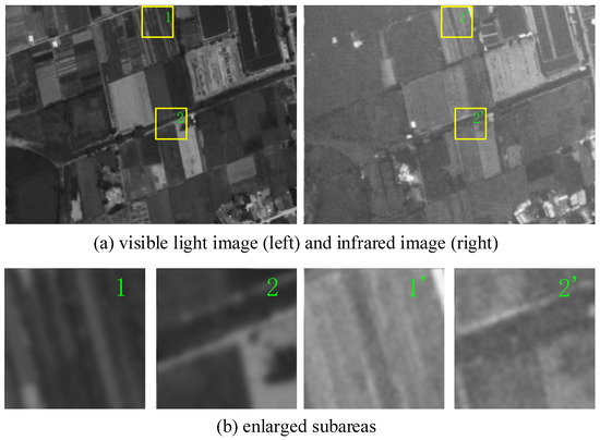
Figure 1.
Cross-modal image pair and their enlarged subareas. Image (a) shows the visible light image and the infrared image captured in a same scene. Image (b) shows the enlarged subareas which are captured and enlarged from the rectangle areas in Image (a).
The matching algorithms developed in [8,11] are very computationally expensive. To solve the problem, the visual odometer based on optical flow [12] combined with particle filter is adopted to restrict the search area of the matching and eliminate the incorrect results [11]. However, optical flow is not drift-free and can be easily interrupted by motion blur or light changes. Consequently, the position solution is still unstable if both the image matching and the visual odometer produce unreliable input.
Deep learning-based image matching method is employed in [3] for UAV localization; however, the precision of the image matching algorithm is very low to estimate the precise heading of the UAV, which means that the heading estimation from the image matching cannot be used to correct the INS heading. Therefore, only INS position can be corrected by the image matching results. Finally, these image matching methods [3,8,11] are developed mainly for the visible light images, which means their visual positioning methods only work in daylight.
In the last decade, vision-based simultaneous localization and mapping (VSLAM) has been extensively studied [11,13]. However, pure vision-based SLAM is usually not a robust solution for navigation. The main drawback of VSLAM is that the vision tracker could be easily interrupted by light change, motion blurring, or occlusion of moving objects. For solving this problem, vision and inertial fusion-based SLAM (VISLAM) has been proposed [14,15]. VISLAM is more robust than VSLAM since the inertial module would not be affected by light change, motion blurring, or occlusion, which can consistently provide the motion states to the navigation system [16,17,18]. Meanwhile, the vision system can provide environmental perception and states correction, which is supplemental to the internal module. Nevertheless, the VISLAM suffers from the position drift problem. Therefore, closed-loop optimization is employed for correcting the drift [15,19]. However, the long path closed-loop optimization is very expensive in both computation and memory consumption. In addition, closed-loop path is not always available for UAVs navigation, for example, for single-way flying of UAVs. Although VISLAM has been widely and successfully used for indoor (or enclosed environment) navigation, it is still very hard to apply for UAV navigation in large open environment.
In this paper, we proposed an airborne MEMS INS enhancing method based on cross-modal images matching, which can provide long range autonomous navigation for medium- and high-altitude aircraft under GNSS blocking environment. The main contributions of this work are the following:
- (I)
- A coarse matching algorithm based on the dense structure features is proposed to effectively adapt to nonlinear grayscale variation and noise distortion. In addition, the searching process of the coarse matching is significantly accelerated with fast Fourier transform (FFT). Therefore, the proposed coarse matching algorithm can provide position updates with a rate above 10 Hz on a low power airborne compute. Since the proposed coarse matching method is reliable and time efficient, the visual odometer is no longer required.
- (II)
- A fine alignment algorithm based on a deep end-to-end trainable matching network is proposed to precisely align the real-time aerial image with the referenced satellite image despite the local ground feature changes and nonlinear grayscale variation. The result of fine alignment is employed to estimate the precise heading angle of the UAV, which is better than three degrees (1σ) during a typical experiment and can be used to correct the heading angle of the MEMS INS.
- (III)
- Based on the cross-modal image matching approach, a precise position and heading can be obtained, which is used to enhance the MEMS INS performances in this research. A filtering model to fuse the vision-based navigation information and the INS information is developed, which can precisely and reliably estimate the position, velocity, and attitude errors of the UAV and avoid the accumulating errors of the MEMS INS. The enhanced navigation approach can provide long-time autonomous navigation for the UAV at medium- to high-altitude at GNSS denied environments, and it can work effectively in both daylight condition (with visible light camera) and night condition (with infrared camera).
In the remaining parts of this paper, Section 2 describes the cross-modal image matching approach to achieve the position and heading enhancement information. The data fusion approach to achieve the enhancement to MEMS INS with image matching is discussed in Section 3. The experimental tests are discussed in Section 4, and the concluding remarks are provided in Section 5.
2. Position and Heading Estimation Approach Based on Cross-Modal Image Matching
The overall scheme of the proposed visual estimator is shown in Figure 2. The camera calibration is realized with OpenCV camera calibration module [20]. Before the image matching, the real-time image is corrected according to the pose, altitude, and the parameters of the camera. After the correction, the ground resolution and the orientation of the real-time image and the referenced image are significantly the same. The transition of the real-time image relative to referenced image can be estimated by the coarse matching.
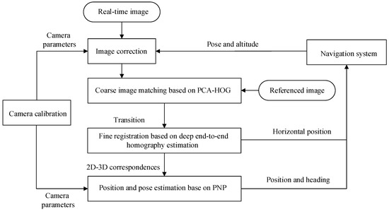
Figure 2.
Flowchart of the proposed visual estimator.
After the image correction, the center point of the corrected image is directly below the aircraft. Therefore, the horizontal position of the UAV can be directly calculated according to the result of the coarse matching.
The result of the coarse matching is then inputted into the fine alignment algorithm, which will estimate the homography transformation between the real-time image and the referenced image. Precise point correspondences between the real-time image and the referenced image can be produced with the homography transformation. The points in the referenced image can be mapped to the world coordinate system with zero height. Therefore, correspondences between the 2D point in the real-time image and 3D point in the world coordinate system are established. Then, the position (relative to the ground) and pose of the camera can be calculated with perspective-n-point (PNP) method [21] according to the 2D to 3D point correspondences and the camera parameters provided by the calibration. Finally, the position and heading estimated is sent to the INS for performance enhancement.
2.1. Fast Coarse Image Matching Based on PCA-HOG
2.1.1. PCA-HOG Feature Description
Histogram of oriented gradient (HOG) is a common feature descriptor used in target detection and image matching. HOG is a description based on the statistics of local gradient magnitude and direction, which has good invariability for grayscale variation [22]. However, HOG is very sensitive to the noise distortion since it is formed based on gradient direction, which is easily disturbed by the distortion between cross-modal images.
To improve the noise reliability, we employ principal component analysis (PCA) to enhance the local gradient orientation. The PCA is typically used to calculate the dominant vectors of a given dataset that can reduce the noise component in signals and estimate the local dominant orientation.
For each pixel, the PCA can be applied to the local gradient vectors to obtain their local dominant direction.
Given the original image I with its horizontal derivative image and vertical derivative image , an local gradient matrix is constructed for each pixel:
They can be calculated with Sobel calculators [23]. is determined by the size of the local window of the PCA calculation. For example, if the size of the window for each pixel is , then the value of is 9.
The dominant orientation can be estimated by determining a unit vector perpendicular to the combined direction of the local gradient vectors . Since the production of vectors perpendicular to each other is 0; therefore, this can be formulated as the following minimization problem:
Vector can be solved by applying SVD to the local gradient matrix :
where is an orthogonal matrix, is an matrix, is a orthogonal matrix, and indicates the local dominant orientation of the local gradient.
The PCA enhanced structure orientation can be calculated according to the following equation:
where , is the element in the first row of and is the element in the second row of . Note that the structure orientation is orthogonal to the orientation of the gradient vector.
The orientation enhanced by PCA is more robust against the distortion between cross-modal images than the orientation directly estimated with local gradient. Figure 3a,b shows two examples of comparing gradient orientation and PCA enhanced ordination. Clearly, PCA enhanced ordination is more stable under the cross-modal distortion.
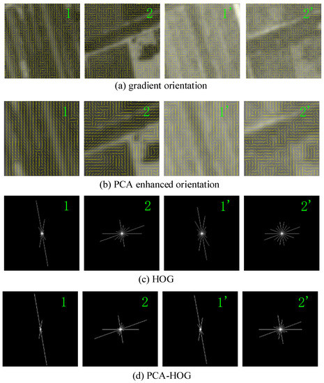
Figure 3.
Examples of comparing gradient orientation and PCA-enhanced ordination. The numbers in the top right of the image indicate the orientation maps or the descriptions that are extracted from the enlarged subareas from the cross-modal image pairs provided in Figure 1.
The PCA-HOG description is a feature vector, which is calculated at each pixel of image. The PCA-HOG description and the HOG description [22] are calculated in the same procedure, except that the local gradient orientation is replaced by the PCA enhanced orientation. The examples of comparing PCA-HOG and HOG are provided in Figure 3c,d. We can see that cross-modal distortion causes more significant change to the patterns of HOG descriptor compared with the patterns of PCA-HOG descriptor.
2.1.2. Searching Process Accelerating
Coarse matching is a full-searching template matching as shown in Figure 4. The template, namely, the aforementioned corrected real-time image, needs to be compared with each candidate window in the referenced image and matched to the most similar window. The similarity of PCA-HOG can be calculated with the sum of squared differences (SSD) as follows:
where represents the PCA-HOG feature vector of the pixel in , and is the transition between the template and the corresponding candidate window in the referenced image.
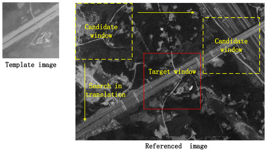
Figure 4.
Example of full-searching template matching with cross-modal images, the template image is a real-time infrared image and the referenced image is a satellite visible light image.
However, the searching process with per-pixel SSD calculation is very computationally expensive. To reduce the computational burden, we developed a fast convolution-based method for the template searching. First, we define the similarity of PCA-HOG feature map as the following equation:
where the operator represents the dot product, and is the normalized (by L2 norm) PCA-HOG feature vector of the pixel in . Then, the full-searching process can be defined as the following convolution:
where is the transition between the template and the referenced image estimate by the searching process. The convolution can be accelerated in frequency domain by using fast Fourier transform (FFT):
where is fast Fourier transform, is the complex conjugate of , and is inverse fast Fourier transform (IFFT). IFFT and FFT are the main parts of the computation of the accelerated convolution process. Suppose the size of the template is and the size of the referenced image is . The computation complexity of the searching process with SSD is , while the computation complexity of the searching process accelerated with FFT is O(2m2logm). The accelerating ratio is varied with the size of image, which is given in Table 1 by examples. We can see that a significant computation decrease can be achieved by the accelerating method.

Table 1.
Computation comparison of the two search methods.
2.2. Fine Alignment Based on End-to-End Trainable Matching Network
Fine alignment for cross-modal images is very challenging due to the complicated grayscale variation and the local ground feature changes. The image matching methods based on handcrafted features have very limited ability for addressing the challenges [10,24].
Rocco et al. [24] proposed an image matching method based on convolutional neural network (CNN) for both instance-level and category-level matching, which can handle substantial appearance differences, background clutter, and large deformable transformation. Based on this method, Park et al. [10] proposed a two-stream symmetric network for aerial image matching which can adapt to the light change and the variation of ground appearance, and the matching precision is further improved in paper [25]. However, the matching precision of these methods is low, mainly due to the lower resolution of the input image and the lower resolution of the features extraction, as pointed out in paper [24].
2.2.1. Loss Function
Suppose the ground truth homography transformation between a real-time image and a referenced image is , and the homography transformation estimated between the subareas of this training pair is , then the loss function is calculated by the following:
where is the number of grid points, and is the translation between the subarea and the real-time image, as shown in Figure 5. The loss function is based on the transformed grid loss proposed in [24], which minimizes the discrepancy between the estimated transformation and the ground truth transformation.
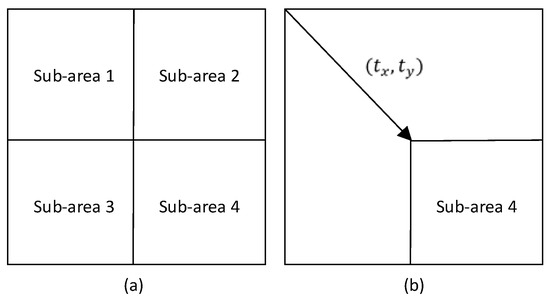
Figure 5.
Image partition. Image (a) shows that the input image is divided into four subareas. In image (b), the arrow indicates the translation between the four subareas and the real-time image.
2.2.2. Implementation Details and Discussion
The network is developed based on [24] which is originally trained on visible light images. Therefore, we build a training dataset with 5000 pairs of infrared aerial image and visible light satellite image. We generate the ground true pairs by applying homography transformation to the manually aligned pairs, since there are no datasets with completely correct transformation parameters between infrared aerial image and visible light satellite image.
The resolution of the input image is 640 × 480. The input image will be divided into four subareas and each subarea is then resized to 240 × 240. The feature map is extracted with ResNet-101 network [26] rather than VGG-16 network [27], since the former achieves better matching performance as reported in [28].
The partition approach increases the resolution of the input image and the resolution of the features extraction, which helps in improving the matching precision. Of course, one can also enhance the precision by inputting the image with high resolution rather than using partition, but that may introduce an enormous increase in parameters to the network, which makes the retraining process (for cross-modal images) difficult and eventually lowers the performance of the inference.
In the partition approach, the four subarea pairs share the backbone network and the regression network, which means the number of the parameters of the network is not increased. This facilitates the retraining process and the deployment of network, which will eventually enhance the performance of the homography estimation with a modest training dataset.
During the inference, the global homography transformation for the fine alignment is estimated with RANSAC algorithm [29], which minimizes the re-projection errors of the four homography transformations of the subarea pairs.
Examples of the coarse matching and the fine alignment are shown in Figure 6. We can see that the features in the results of fine alignment are aligned more accurately compared with the results of coarse matching.
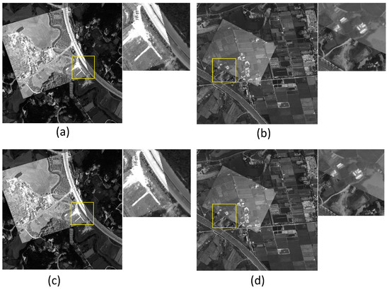
Figure 6.
Results of coarse matching and fine alignment. Image (a,b) shows the results of coarse matching. Image (c,d) shows the results of fine alignment. The areas in the windows in these results are enlarged and given in the top right.
3. Enhancement of MEMS INS for UAV Navigation
3.1. Overall Scheme
According to the above discussion, the drift-free position and heading of the UAV can be calculated from the cross-modal image matching, in which the information will be used to enhance the MEMS INS to improve the autonomous navigation performance of UAV.
INS obtains the position, velocity, and attitude of the UAV by integrating the acceleration and angular rate from the accelerometers and gyros, respectively. However, the navigation errors of the INS will accumulate due to the drifts of the accelerometers and the gyros used [30,31], which is especially challenging for the MEMS INS due to the unstable characteristics of the MEMS inertial sensors [1,2]. The cross-modal image matching is used to enhance the performance of the MEMS INS herein. The overall scheme is shown in Figure 7, and the main steps are as follows:
- (I)
- The real-time images from the camera mounted in the UAV are transformed and corrected by the reference attitude from the MEMS INS initially, and then from the extended Kalman filter which will be discussed below.
- (II)
- The transformed real-time images are used to match with the geo-referenced images, which is pre-prepared and stored in the UAV navigation computer before the task, and obtain the position and heading of the UAV by solving the PNP pose as discussed in Section 2.
- (III)
- The MEMS INS position, velocity, attitude, and heading are calculated by the inertial navigation algorithm.
- (IV)
- An extended Kalman filter is designed to fuse the navigation data from image matching and from MEMS INS.

Figure 7.
Integrated navigation algorithm overall scheme.
The system model and measurement model for data fusion are derived, respectively. The extended Kalman filter compares the navigation results from the image matching and from MEMS INS, and estimates and corrects the position, velocity, attitude errors, and compensates the drifts of the inertial sensors.
3.2. System Model for Data Fusion
The SINS error model is commonly used by the design of Kalman filter model. In this proposed system, the errors are always defined in the navigation frame. First, we choose the local-level geographic frame as the navigation frame, which is denoted as n frame. Then, the body frame is defined as b frame, which is aligned with its longitudinal, lateral, and vertical axes.
The attitude error equation of INS is defined as follows [32,33]:
where refers to the attitude error vector projected in navigation frame, refers to the rotation rate of the navigation frame with respect to the inertial frame, represents the attitude matrix from the body frame to the navigation frame, and refers to the gyro bias vector in the navigation frame.
The velocity error equation of INS is defined as follows [32,33]:
where represents the velocity error in the navigation system, refers to the rotation rate of the earth frame with respect to the inertial frame, is the specific force projected in the navigation frame, and represents the accelerometer zero bias expressed in the navigation frame.
The position error equation of INS is defined as follows [32,33]:
where is the position error in the navigation system.
The biases of the gyroscopes and accelerometers can be regarded as a constant within a certain period of time, and they are modeled as follows:
Based on the above INS error model, we select the attitude error, velocity error, position error, biases of the gyroscopes and accelerometers as the states of the data fusion filter. This yields a 15-element state vector :
Considering Equations (11)–(15), the state equation of the data fusion filter can be written as follows:
where is the 15-dimension state noise variance vector, and the system matrix can be expressed as follows:
The submatrix in system matrix can be expressed as follows:
3.3. Measurement Model for Data Fusion
In our research, the measurement information comes from the image matching observations as discussed in Section 2, and this information is used to correct the MEMS INS degradation with time by the Kalman filtering mechanism.
The image matching procedure can provide position, attitude, and heading observations. However, considering that the attitude observation from image matching is generally at the level of a few tenths of a degree; therefore, it is not accurate enough for correcting the attitude of MEMS INS. As a result, in this research, the position and heading observations from image matching are chosen as the measurements for Kalman filter of data fusion.
For the aircraft position measurement, define as the position obtained from the image matching, and as the position obtained from the MEMS INS. Therefore, the position error of the inertial navigation can be expressed as follows:
Considering the definition of the state vector X in Equation (15), the above position error can be expressed as:
where the coefficient matrix can be expressed as:
For the aircraft heading measurement, define as the heading angle obtained from the image matching, and as the heading angle obtained from the MEMS INS. Therefore, the heading error of the inertial navigation can be expressed as follows:
Herein, to construct the measurement model for the data fusion Kalman filter, we also need to provide the relation between the heading error and the state vector X, as in Equation (20). However, the relation between the heading error and the state vector X is not very straightforward. The heading error described in Equation (22) is defined as the Euler error; however, the heading error component in state vector X is defined as the mathematical platform error [33]. Their relation can be derived as follows:
As discussed in the previous sections, represents the attitude matrix from the body frame to the navigation frame, which can be expressed as follows if are defined to be the heading, pitch, and roll, respectively [34].
For brevity, we use to denote the element of in row and column . Therefore, the heading angle can be calculated from as:
The heading error can be obtained from the variation of Equation (24), and can be expressed as follows:
In Equation (25), are the elements of the attitude error matrix , which can be calculated as:
where is defined as the attitude matrix from the body frame to mathematical platform , and it can be calculated as follows:
In Equation (27), represents the attitude matrix from the navigation frame to mathematical platform , and it can be calculated by using the platform attitude error vector in Equation (15) as follows [33]:
where are the components of projected in navigation frame .
Combine Equations (16)–(18) into (15), and the heading error can be expressed as follows:
Compared with Equation (22), it can be found that the following relationship holds:
Consider the definition of state vector X, the following equation can be obtained:
where is defined as follows according to Equation (29):
Define as the coefficient matrix of Equation (31), and the attitude error equation can be expressed as follows:
Combine Equations (20) and (31), the measurement model for data fusion can be obtained as follows:
where the measurement model coefficient matrix can be expressed as follows:
4. Experimental Tests
4.1. Test Conditions
The proposed enhanced navigation approach is evaluated by field tests. In these tests, a visible light camera and an infrared camera are carried by the UAV (DJI M600Pro made by DJI Technology Co., Ltd. in Shenzhen, China) to capture the real-time aerial image, as shown in Figure 8. All the data of the sensors are real-timely collected and processed by an onboard computer (Jetson Nano made by NVIDIA Corp. in Beijing, China), which has a CPU composed of 4-core ARM A57 @1.43 GHz and a GPU composed of 128-core Maxwell @912 Hz.
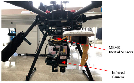
Figure 8.
The flying tests platform.
The visible light and the infrared camera parameters are listed in Table 2, and the MEMS inertial sensor parameters are shown in Table 3.
Table 2.
Camera parameters.
Table 3.
MEMS inertial sensor parameters.
4.2. Test Results
The proposed cross-modal image matching approach (CMM) is compared with HOP [11], which combines histograms of oriented gradients (HOG), optical flow (OF), and particle filter (PF). HOP uses a matching method based on HOG for positioning, and, to accelerate the matching process, OF and PF are employed to decrease the searching area.
The positioning accuracy of CMM and HOP is evaluated by comparing their positioning results with the GPS RTK, which generally has an accuracy of 0.02 m under benign environments.
The correct positioning ratio (CPR) is selected for evaluating the positioning reliability of CMM and HOP. Herein, the CPR is defined as , where is the total number of positioning, and is the correct number of positioning. According to the positioning requirement of the UAV, herein, we define that a positioning result is correct if its error is less than 30 m compared with the GPS RTK. The root-mean-squares error (RMSE) of the correct positioning is selected for evaluating the positioning accuracy.
Eight UAV flights are carried out to evaluate the aforementioned approaches, namely, CMM and HOP. The flight parameters are provided in Table 4. The flight trajectories are shown in Figure 9. The correct positioning ratio and the positioning RMS error of CMM and HOP are compared in Table 5.
Table 4.
UAV flight parameters.
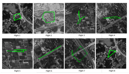
Figure 9.
The flight trajectory of the eight flights.
Table 5.
CMM and HOP performance comparison.
It can be noted from Table 5 that both the CPR and positioning accuracy of HOP are significantly lower than those of CMM for all the flights. There are mainly two reasons for the low performances of HOP. First, the image matching algorithm of HOP is developed for visible light images, which is unreliable for matching cross-modal images; therefore, its CPRs are very low in the flights with infrared camera. Second, the searching area of HOP is small (about 30 m × 30 m) due to the high computation complexity of the matching; therefore, the true position could be out of the searching area when a false prediction is introduced by a false matching.
Furthermore, the contribution of the coarse matching of CMM can be observed by comparing the CPR of HOP with that of CMM. The feature descriptor of the proposed coarse matching is enhanced by PCA, which is more reliable for matching cross-modal images. In addition, the searching process of the coarse matching of CMM is significantly accelerated, which means we can afford a significantly larger searching area . Therefore, the CMM can re-track the flight path even when the true position is far from the predict position, which also helps in improving the reliability of CMM. Table 6 shows the time-consuming statistics of CMM, where the visible light real-time image is resized from 2048 × 2048 pixels to 512 × 512 pixels. Since the ground resolution of visible light real-time image is significantly higher than the reference image, we can save the computation without losing the position precision by decreasing the resolution of real-time image properly. From the statistics of Table 6, it can be noted that the proposed coarse matching algorithm can realize an average position update rate of 12.6 Hz (79.1 ms) for infrared image, and an average position update rate of 12.1 Hz (82.6 ms) for visible light.
Table 6.
Time-consuming statistics of CMM.
The positioning and heading obtained from the image matching are finally used to enhance the MEMS INS in order to improve the autonomous navigation performance of UAV according to the approach proposed in Section 3. Herein, the positioning and heading results of CMM and those of HOP are separately used to aid the MEMS INS, whose raw sensors data are collected during the flying tests.
The CMM enhanced MEMS INS positioning errors are shown in Figure 10, and the comparative HOP enhanced MEMS INS positioning errors are shown in Figure 11. By comparing Figure 10; Figure 11, it can be seen that both the positioning accuracy and the positioning stability are improved dramatically. It can be noted that there exists some error “jumps” in Figure 11 during the HOP enhanced MEMS INS process. This phenomenon arises from the fact that the HOP imaging matching approach has a low CPR, which affects the integration of HOP and MEMS INS. The statistics of the enhanced MEMS INS positioning results are listed in Table 7, which shows that the CMM enhanced system achieves significantly better performances than the HOP enhanced system.
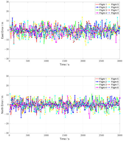
Figure 10.
CMM enhanced MEMS INS positioning errors.
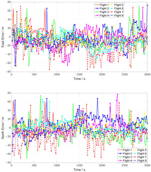
Figure 11.
HOP enhanced MEMS INS positioning errors.
Table 7.
CMM and HOP enhanced MEMS INS performance comparison.
5. Concluding Remarks
In this paper, we proposed a novel, practical, and robust UAV navigation method. A novel cross-modal image matching method is proposed to efficiently and reliably match the aerial infrared image or aerial visible light image with the visible light satellite image.
With the enhancement of the proposed cross-modal image matching method, our navigation method can provide long-time autonomous navigation for the UAV at GNSS denied environments, and it can work effectively in both daylight and night conditions.
In addition, our method can efficiently run at a lower power common embedded platform and the experimental tests show that the states estimation is reliable and precise enough for most applications with UAVs.
The real-time image has to be rectified before the coarse image matching, which means the proposed method cannot be applied to the system with uncalibrated camera. In addition, the attitude of the camera with a standard error of less than 3 degrees is required for real-time image rectification.
In the future work, we will focus on enhancing the precision of the positioning and improving the weather adaptability of the algorithm.
Author Contributions
Conceptualization, S.H. and J.D.; methodology, S.H., J.D. and A.S.; software, S.H. and J.D.; validation, S.H., J.D. and K.W.; formal analysis, K.W.; investigation, S.H. and M.Z.; resources, S.H.; data curation, M.Z.; writing—original draft preparation, M.Z. and K.W.; writing—review and editing, S.H. and J.D.; visualization, M.Z.; supervision, S.H.; project administration, J.D.; funding acquisition, S.H. and J.D. All authors have read and agreed to the published version of the manuscript.
Funding
This work was supported in part by the National Natural Science Foundation of China with Grant number 61203199; and in part by the National Natural Science Foundation of China with Grant number 61802423.
Institutional Review Board Statement
Not applicable.
Informed Consent Statement
Not applicable.
Data Availability Statement
There are no new data is created.
Conflicts of Interest
The authors declare no conflict of interest.
References
- Tomczyk, A.M.; Ewertowski, M.W.; Stawska, M.; Rachlewicz, G. Detailed alluvial fan geomorphology in a high-arctic periglacial environment, Svalbard: Application of unmanned aerial vehicle (UAV) surveys. J. Maps 2019, 15, 460–473. [Google Scholar] [CrossRef]
- Shakhatreh, H.; Sawalmeh, A.H.; Al-Fuqaha, A.; Dou, Z.C.; Almaita, E.; Khalil, I.; Othman, N.S.; Khreishah, A.; Guizani, M. Unmanned Aerial Vehicles (UAVs): A Survey on Civil Applications and Key Research Challenges. IEEE Access 2019, 7, 48572–48634. [Google Scholar] [CrossRef]
- Zhang, Y.; Ma, G.; Wu, J. Air-Ground Multi-Source Image Matching Based on High-Precision Reference Image. Remote Sens. 2022, 14, 588. [Google Scholar] [CrossRef]
- Jahromi, A.J.; Broumandan, A.; Daneshmand, S.; Lachapelle, G.; Ioannides, R.T. Galileo signal authenticity verification using signal quality monitoring methods. In Proceedings of the 2016 International Conference on Localization and GNSS (ICL-GNSS), Barcelona, Spain, 28–30 June 2016; pp. 1–8. [Google Scholar]
- Sivaneri, V.O.; Gross, J.N. UGV-to-UAV cooperative ranging for robust navigation in GNSS-challenged environments. Aerosp. Sci. Technol. 2017, 71, 245–255. [Google Scholar] [CrossRef]
- Kim, Y.; Hwang, D.-H. Vision/INS Integrated Navigation System for Poor Vision Navigation Environments. Sensors 2016, 16, 1672. [Google Scholar] [CrossRef] [PubMed]
- Mikov, A.; Cloitre, A.; Prikhodko, I. Stereo-Vision-Aided Inertial Navigation for Automotive Applications. IEEE Sens. Lett. 2021, 5, 1–4. [Google Scholar] [CrossRef]
- Yol, A.; Delabarre, B.; Dame, A.; Dartois, J.É.; Marchand, E. Vision-based absolute localization for unmanned aerial vehicles. In Proceedings of the 2014 IEEE/RSJ International Conference on Intelligent Robots and Systems, Chicago, IL, USA, 14–18 September 2014; pp. 3429–3434. [Google Scholar]
- Ye, Y.X.; Shan, J.; Bruzzone, L.; Shen, L. Robust Registration of Multimodal Remote Sensing Images Based on Structural Similarity. IEEE Trans. Geosci. Remote Sens. 2017, 55, 2941–2958. [Google Scholar] [CrossRef]
- Park, J.H.; Nam, W.J.; Lee, S.W. A Two-Stream Symmetric Network with Bidirectional Ensemble for Aerial Image Matching. Remote Sens. 2020, 12, 20. [Google Scholar] [CrossRef]
- Shan, M.; Wang, F.; Lin, F.; Gao, Z.; Tang, Y.Z.; Chen, B.M. Google map aided visual navigation for UAVs in GPS-denied environment. In Proceedings of the 2015 IEEE International Conference on Robotics and Biomimetics (ROBIO), Zhuhai, China, 6–9 December 2015; pp. 114–119. [Google Scholar]
- Barron, J.L.; Fleet, D.J.; Beauchemin, S.S.; Burkitt, T.A. Performance of optical flow techniques. In Proceedings of the 1992 IEEE Computer Society Conference on Computer Vision and Pattern Recognition, Champaign, IL, USA, 15–18 June 1992; pp. 236–242. [Google Scholar]
- Lai, T. A Review on Visual-SLAM: Advancements from Geometric Modelling to Learning-Based Semantic Scene Understanding Using Multi-Modal Sensor Fusion. Sensors 2022, 22, 7265. [Google Scholar] [CrossRef]
- Qin, T.; Li, P.; Shen, S. VINS-Mono: A Robust and Versatile Monocular Visual-Inertial State Estimator. IEEE Trans. Robot. 2018, 34, 1004–1020. [Google Scholar] [CrossRef]
- Qin, T.; Li, P.; Shen, S. Relocalization, Global Optimization and Map Merging for Monocular Visual-Inertial SLAM. In Proceedings of the 2018 IEEE International Conference on Robotics and Automation (ICRA), Brisbane, Australia, 21–25 May 2018; pp. 1197–1204. [Google Scholar]
- Bai, J.; Gao, J.; Lin, Y.; Liu, Z.; Lian, S.; Liu, D. A Novel Feedback Mechanism-Based Stereo Visual-Inertial SLAM. IEEE Access 2019, 7, 147721–147731. [Google Scholar] [CrossRef]
- Coulin, J.; Guillemard, R.; Gay-Bellile, V.; Joly, C.; Fortelle, A.d.L. Tightly-Coupled Magneto-Visual-Inertial Fusion for Long Term Localization in Indoor Environment. IEEE Robot. Autom. Lett. 2022, 7, 952–959. [Google Scholar] [CrossRef]
- Gurturk, M.; Yusefi, A.; Aslan, M.F.; Soycan, M.; Durdu, A.; Masiero, A. The YTU dataset and recurrent neural network based visual-inertial odometry. Measurement 2021, 184, 109878. [Google Scholar] [CrossRef]
- Mur-Artal, R.; Montiel, J.M.M.; Tardós, J.D. ORB-SLAM: A Versatile and Accurate Monocular SLAM System. IEEE Trans. Robot. 2015, 31, 1147–1163. [Google Scholar] [CrossRef]
- Wang, Y.M.; Li, Y.; Zheng, J.B. A camera calibration technique based on OpenCV. In Proceedings of the 3rd International Conference on Information Sciences and Interaction Sciences, Chengdu, China, 23–25 June 2010; pp. 403–406. [Google Scholar]
- Marchand, E.; Uchiyama, H.; Spindler, F. Pose Estimation for Augmented Reality: A Hands-On Survey. IEEE Trans. Vis. Comput. Graph. 2016, 22, 2633–2651. [Google Scholar] [CrossRef] [PubMed]
- Dalal, N.; Triggs, B. Histograms of oriented gradients for human detection. In Proceedings of the 2005 IEEE Computer Society Conference on Computer Vision and Pattern Recognition (CVPR’05), San Diego, CA, USA, 20–25 June 2005; Volume 881, pp. 886–893. [Google Scholar]
- Nixon, M.S.; Aguado, A. Feature Extraction & Image Processing for Computer Vision, 3rd ed.; Academic Press: Cambridge, MA, USA, 2012; p. 609. [Google Scholar]
- Rocco, I.; Arandjelovic, R.; Sivic, J. Convolutional Neural Network Architecture for Geometric Matching. IEEE Trans. Pattern Anal. Mach. Intell. 2019, 41, 2553–2567. [Google Scholar] [CrossRef]
- Chen, Y.; Zhang, Q.; Zhang, W.; Chen, L. Bidirectional Symmetry Network with Dual-Field Cyclic Attention for Multi-Temporal Aerial Remote Sensing Image Registration. Symmetry 2021, 13, 1863. [Google Scholar] [CrossRef]
- He, K.; Zhang, X.; Ren, S.; Sun, J. Deep Residual Learning for Image Recognition. In Proceedings of the 2016 IEEE Conference on Computer Vision and Pattern Recognition (CVPR), Las Vegas, NV, USA, 27–30 June 2016; pp. 770–778. [Google Scholar]
- Liu, S.; Deng, W. Very deep convolutional neural network based image classification using small training sample size. In Proceedings of the 2015 3rd IAPR Asian Conference on Pattern Recognition (ACPR), Kuala Lumpur, Malaysia, 3–6 November 2015; pp. 730–734. [Google Scholar]
- Rocco, I.; Arandjelovic, R.; Sivic, J. End-to-End Weakly-Supervised Semantic Alignment. In Proceedings of the 2018 IEEE/CVF Conference on Computer Vision and Pattern Recognition, Salt Lake City, UT, USA, 18–23 June 2018; pp. 6917–6925. [Google Scholar]
- Fischler, M.; Bolles, R. Random Sample Consensus: A Paradigm for Model Fitting with Applications To Image Analysis and Automated Cartography. Commun. ACM 1981, 24, 381–395. [Google Scholar] [CrossRef]
- Syed, Z.F.; Aggarwal, P.; Niu, X.; El-Sheimy, N. Civilian Vehicle Navigation: Required Alignment of the Inertial Sensors for Acceptable Navigation Accuracies. IEEE Trans. Veh. Technol. 2008, 57, 3402–3412. [Google Scholar] [CrossRef]
- Grenon, G.; An, P.E.; Smith, S.M.; Healey, A.J. Enhancement of the inertial navigation system for the Morpheus autonomous underwater vehicles. IEEE J. Ocean. Eng. 2001, 26, 548–560. [Google Scholar] [CrossRef]
- Savage, P.G. Strapdown Inertial Navigation Integration Algorithm Design Part 2: Velocity and Position Algorithms. J. Guid. Control Dyn. 1998, 21, 208–221. [Google Scholar] [CrossRef]
- Savage, P.G. Strapdown Inertial Navigation Integration Algorithm Design Part 1: Attitude Algorithms. J. Guid. Control Dyn. 1998, 21, 19–28. [Google Scholar] [CrossRef]
- Yuan, W.; Gui, M.; Ning, X. Initial Attitude Estimation and Installation Errors Calibration of the IMU for Plane by SINS/CNS Integration. In Proceedings of the 2017 Chinese Intelligent Automation Conference, Tianjin, China, 2–4 June 2017; pp. 123–130. [Google Scholar]
Disclaimer/Publisher’s Note: The statements, opinions and data contained in all publications are solely those of the individual author(s) and contributor(s) and not of MDPI and/or the editor(s). MDPI and/or the editor(s) disclaim responsibility for any injury to people or property resulting from any ideas, methods, instructions or products referred to in the content. |
© 2023 by the authors. Licensee MDPI, Basel, Switzerland. This article is an open access article distributed under the terms and conditions of the Creative Commons Attribution (CC BY) license (https://creativecommons.org/licenses/by/4.0/).