Article

Spectrum-Based Logistic Regression Modeling for the Sea Bottom Soil Categorization

Civil Engineering Department, Sami Shamoon College of Engineering, Ashdod 77245, Israel
*
Authors to whom correspondence should be addressed.
Appl. Sci. 2023, 13(14), 8131; https://doi.org/10.3390/app13148131
Submission received: 14 May 2023 / Revised: 28 June 2023 / Accepted: 11 July 2023 / Published: 12 July 2023
(This article belongs to the Collection Nondestructive Testing (NDT))

Abstract

:
The present analysis of state of the art portrays that actual time series or spectrum backscattered data from a point on the sea bottom are rarely used as features for machine learning models. The paper deals with the artificial intelligence techniques used to examine CHIRP-recorded data. The data were collected using a CHIRP sub-bottom profiler to study two sand bottom sites and two sandstone bottom sites in the offshore zone of Ashqelon City (Southern Israel). The first reflection time series and spectra of all the traces from the four sites generated two training and two test sets. Two logistic regression models were trained using the training sets and evaluated for accuracy using the test sets. The examination results indicate that types of sea bottom can be quantitatively characterized by applying logistic regression models to either the backscatter time series of a frequency-modulated signal or the spectrum of that backscatter. The examination accuracy reached 90% for the time series and 94% for the spectra. The application of spectral data as features for more advanced machine learning algorithms and the advantages of their combination with other types of data have great potential for future research and the enhancement of remote marine soil classification.

1. Introduction

Acoustic data are an indispensable marine science tool widely used to map and analyze sea bottom characteristics. This NDT technique is beneficial for soil investigations, which include the use of bathymetric mapping to study the topography of the ocean floor, conducting both shallow and deep acoustic surveys to gain insights into the subsoil, identifying existing infrastructure both on and beneath the seafloor, and determining underwater positioning [1,2,3,4,5,6,7,8,9,10,11,12]. The marine industry relies heavily on calibrated backscatter intensity to classify the composition of the sea bottom’s upper layer using remote sensing tools that have become standard in the field.
Reviewing the scientific literature indicates that research in the field of spectral analysis of the acoustic response of the seafloor is relatively limited, and the focus is on large-scale data and non-localized side-scan data. Single-beam types of sonars, such as sub-bottom profilers or multibeam sonars, are rarely studied. While some studies have explored signal and image processing techniques, occasionally in combination with AI algorithms, a reliable quantitative classification method has not yet been established [13,14,15,16,17,18,19,20,21,22,23,24,25,26,27,28]. Other studies have focused on calibrated backscattering intensity methods [29,30] and sometimes use a subsurface profilometer for geological background [31].
The available literature indicates that the primary means of assessing sub-bottom soil composition in acoustic seabed studies is through backscatter intensity, as exemplified by [32], which often requires extensive calibration, such as that provided by the geocoder algorithm [33]. A comprehensive review conducted by Anderson et al. [34] emphasized the need for careful calibration when attempting to relate acoustic backscattering measurements to the sub-surface properties and contents of the seabed. The few studies [27] that have attempted to identify sea bottom soil types based on spectral characteristics have mostly been limited to side-scan sonar data, which are inherently limited by the scale of the features they capture, as noted by [27]. Moreover, it should be noted that a single swath of acoustic data may comprise multiple soil types, limiting such methods’ applicability. While they may yield valuable insights when applied to large, relatively homogeneous sea bottom regions, they may be less effective when dealing with more complex, heterogeneous areas containing various soil types, such as rock, sand, and clay.
Artificial intelligence (AI) techniques have significantly enhanced acoustic data classification in marine science, providing a more objective and efficient approach to seabed mapping. A study by [35] utilized hybrid artificial neural networks incorporating a self-organizing feature map and learning vector quantization to classify four manganese nodule-bearing sites using angular backscatter intensity as the learning and classification features. The resulting model achieved classification accuracies ranging from 87 to 95%. Additionally, refs. [36,37,38,39] utilized a feedforward neural network and convolutional neural networks to predict source charge and bottom composition (mud and sand combinations) for sus charges. The features varied from simulated pressure time series or extracted features, such as peak level, integrated level, signal length, and decay time, to simulated peak pressure and backscatter intensity. The accuracies of the models varied from 84% to 97% for the convolutional neural network used in [37]. These studies illustrate AI algorithms’ potential in classifying acoustic data for marine soil characterization.
The classification of soil based on multibeam echo sounder (MBES) data has been the focus of recent studies [40,41,42]. One such study, [40], applied support vector machine classification to MBES bathymetric and backscatter data to classify mud, sand, and gravel, achieving an accuracy of 90%. Similarly, [41] utilized deep neural networks to classify the same materials from bathymetric and backscatter data that were reduced using fuzzy ranking. This resulted in an accuracy of 86% for soil classification. Another study [42] achieved a classification accuracy of 93% for mud, sand, and gravel combinations using deep learning with backscatter bathymetry and the angular response and mosaic texture of MBES data. These studies demonstrate the efficacy of AI techniques, specifically support vector machines and deep neural networks, in classifying soil based on MBES data. By incorporating features such as bathymetric and backscatter data, as well as angular response and mosaic texture, the accuracy of soil classification has significantly improved. These findings have important implications for the mapping and characterizing of seabed environments, highlighting the potential of AI techniques for future research in marine science.
Upon analysis of the current state-of-the-art literature, it is evident that the features utilized in machine learning approaches for the topic of this article rely heavily on essential characteristics such as backscatter intensity as a function of the angle of incidence, mosaic texture, and bathymetry [35,36,39,40,41,42]. While these features have proven effective in seabed mapping and classification, it is essential to note that actual time series or spectra backscattered from a point on the seafloor have rarely been utilized. However, a study by [43] demonstrated the potential of using the frequency domain representation of the time series of a reflected chirp sub-bottom profiler signal for distinguishing between sand and sandstone. This approach showed promising results, as the number of crossings of the spectrum at 1/16 of the maximal normalized power classifier demonstrated the ability to assess the probability for sand or sandstone with over 80% certainty in over 75% of the cases. Incorporating this approach into machine learning models for seabed mapping and classification may provide a more comprehensive understanding of the seafloor structures and their associated ecological communities, ultimately leading to the better management and preservation of marine resources. Future research should explore the potential of utilizing time series or spectrum data in machine learning approaches to characterize marine environments, as it may lead to significant advancements in the field.
The central hypothesis of the research [43] was that the spectral features of acoustic signals reflected from sand and sandstone sea bottoms are due to essential dissimilarities in the physical properties of these two media. These properties include low-size morphology at the top of both sediment types, and a discrepancy of several meters (depending on the wave period) beneath the reflector boundary.
As these singularities are significantly different between sand and sandstone, they are expected to affect the acoustic signals reflected from the top of the sea bottom, thus affecting spectral parameters such as amplitude, main frequency, the frequency-dependent reflection coefficient, number of spikes, etc. However, the main disadvantage of the presented method was the qualitative choice of the spectral parameters used for classification resulting in less-than-optimal accuracy.
The present study used the discrete values of the reflected time series and spectra obtained by [43] as training sets for two logistic regression models [44]. This machine learning technique was found to be effective for classifying sand and sandstone. It was shown to equal the results of much more complicated machine learning methods, such as convolutional neural networks, used in previous studies [35,36,37,38,39,40,41,42].
The paper aims to demonstrate that logistic regression models can ensure accurate man-independent promising results (in terms of accuracy) for soil categorization at the sea bottom. As shown below, the suggested method allows us to accurately classify the sand and sandstone, making it a viable and practical option for categorizing these seabed sediment types.
The paper consists of five main sections: Section 2 considers the method of the study, including a description of the experimental setup and data preparation methodology; Section 3 portrays time series and spectral data; Section 4 presents the results of the logistic regression modeling; and Section 5 and Section 6 present our discussion and conclusions.

2. Method

A preliminary data collection was performed using a CHIRP sub-bottom profiler to study two sand bottom sites at 26 m depth and two sandstone bottom sites at 33 m depth, both offshore of Ashqelon. The first reflection time series and spectra of all the traces from the four sites generated two training and two test sets. Two logistic regression models [44] were trained using the training sets, and were evaluated for accuracy using the test sets.

2.1. Experimental Setup

A Bathy-2010PC chirp sub-bottom profiler (SBP) was selected as the acoustic device for the data collection campaign. This instrument’s properties are as follows: a linear chirp with a frequency sweep ranging from 2.75 kHz to 6.75 kHz, a signal duration of 5.4 ms, and a beam angle of 30°. It is anticipated that in this context, the reflected signal will be influenced by the fine-scale morphology of the reflector, such as boulders and sand ripples. The data were collected at two offshore locations near Ashkelon, “Site 1” and “Site 2”, approximately 1.2 km apart. The bottom at Site 1 and Site 2 was previously determined to be sandy, and located at a depth of 26 m. Similarly, data were collected at two other locations, “Site 3” and “Site 4”, about 0.8 km apart. The bottom was determined to be sandstone at 33 m at these sites. The sea bottom’s composition at each site was examined through soil assaying and a drop camera. Each site had an area with similar soil composition that extended several hundreds of meters in radius. The vessel was moored at each site, and its position was slightly adjusted due to wind and wave direction variations during data collection. Each trace was captured at a slightly different location, but over the same soil type. The transducer was installed on the vessel’s side and placed 1 m below the waterline. The sound speed in water was measured to be 1530 m per second. The data were recorded in an unprocessed format without any chirp compression applied. Each trace was captured for 100 milliseconds, encompassing the transmitted signal, the water column, the bottom, and approximately 120 m of soil penetration. The transmission parameters used are summarized in Table 1.

2.2. Data Extraction and Preparation

The SegY files collected during the offshore campaign were utilized to extract data for further analysis. Data extraction was conducted using the SegyMat subroutines package running in Octave 8.0.2. GNU Octave is a high-level language primarily intended for numerical computations. It provides a convenient command line interface for numerically solving linear and nonlinear problems and performing other numerical experiments using a language compatible principally with Matlab (Vers. R2022, The MathWorks, Inc., Natick, Lakeside Campus, 1 Lakeside Campus Drive, Natick, MA 01760, USA). It may also be used as a batch-oriented language. GNU Octave is also freely redistributable software. You may redistribute and modify it under the terms of the GNU General Public License (GPL), as published by the Free Software Foundation. SegyMAT is a Matlab/Octave m-files set used to read and write SEG Y data following SEG Y Revision 0 and 1. The Segymat package can be downloaded from SourceForge and added to the Octave path. Specifically, the ReadSegy function imports the seismic data into a 2D array of the size (number of samples) × (number of traces). To ascertain that soil characteristics, not changes in the transmitted signal, are responsible for differences in the reflected signal, repeatability checks were conducted for all traces across all four sites. The results showed the near-perfect repeatability of the transmitted signal. The time series was then divided into transmitted reverberations, the first reflection, and the remaining signal parts, focusing on the first reflection to characterize the first soil layer. The first reflection was extracted from each trace by identifying the first reflection’s start point as the beginning of a sharp increase in the growth rate of local extremum values, and by setting the first reflection’s duration to that of the transmitted signal. The first reflection (of the time series and spectrum) was then taken as a dataset and used to construct the design matrices.

3. Datasets

The data used in this study consist of time series data and spectral data. Within each category, a training set (design matrix) is used to train the model and find the optimal parameters. In addition, there is a test set, which consists of additional data and is used to assess the performance of the trained model. The training sets include 300 traces collected over the sand from both sand sites, and 150 traces collected over sandstone from both sandstone sites. The test sets include 100 traces collected over the sand from both sand sites, and 50 traces collected over sandstone from both sandstone sites. Traces within the training set are randomly ordered.

3.1. Time Series Data
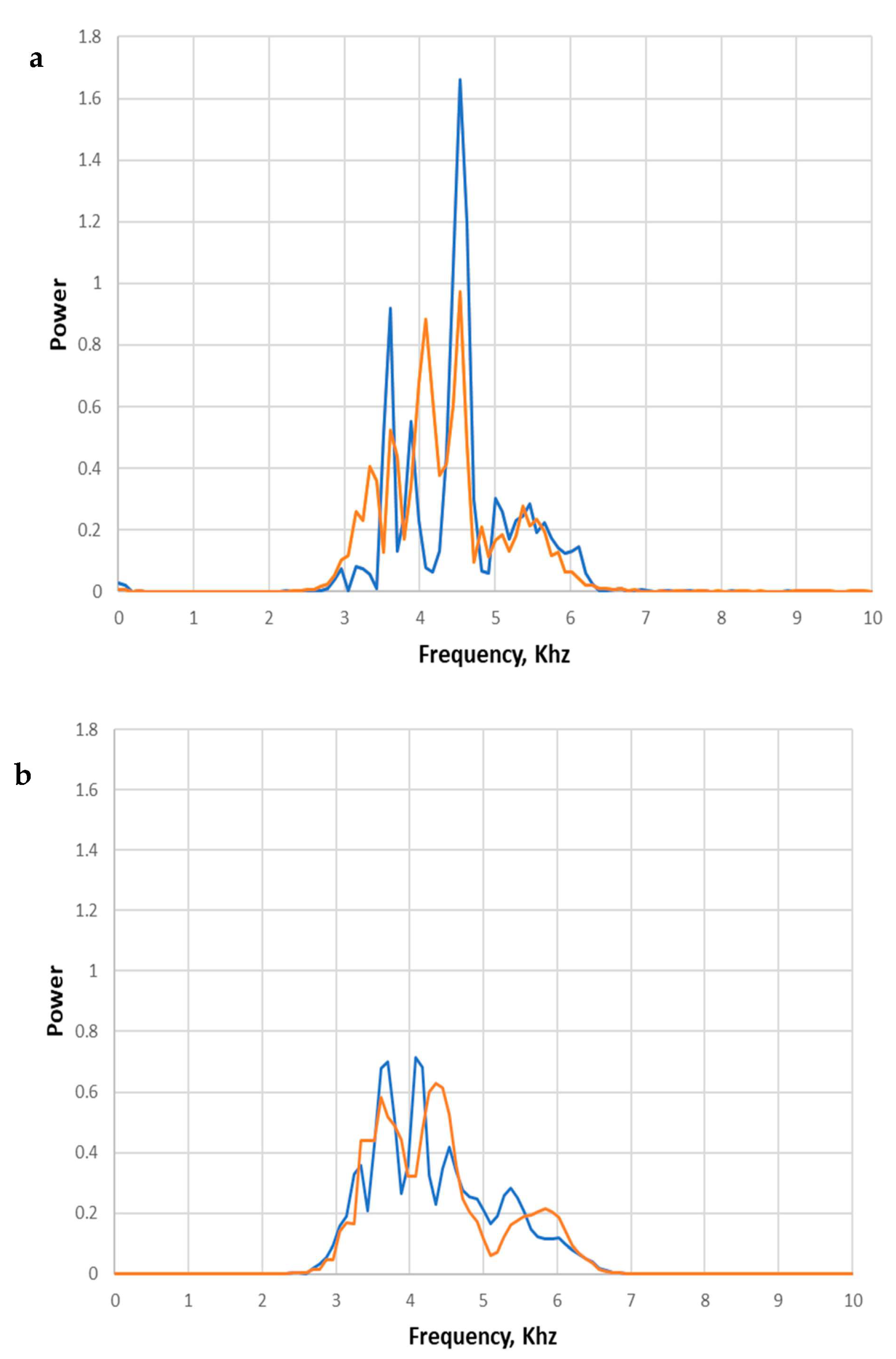
For the time series data, each training (and test) example consists of 108 features corresponding to the raw measurements of the 5.4 ms reflected signal (with a sampling frequency of 20 kHz). Typical time series appear in Figure 1.

3.2. Spectral Data

Obtaining spectral features from acoustic signals reflected from the sea bottom involved several stages, as follows:
  • The time series were auto-correlated and transformed into the frequency domain using the discrete Fourier transform. This results in a two-sided power spectrum containing information on the frequency components of the signal;
  • The positive frequency range was selected to obtain the one-sided power spectrum;
  • The power values were multiplied by two (except for the first term) and normalized by the spectrum area. The normalization step is necessary to correct for differences in attenuation between sand and sandstone sites due to the depth differences;
  • To ensure that the spectra data are clean and accurate, a noise reduction step was performed by applying a frequency bandwidth filter to match the transmitted signal’s frequency range of 2.75 kHz to 6.75 kHz. The resulting discrete spectra points were used as features in machine learning models to classify sand and sandstone sea bottoms.
The spectral datasets (the training and test) were derived from the time series datasets used in the study, and hence included the same composition of sand and sandstone reflections as the time series data. Examples for the stacked power spectra for the four sites appear in Figure 2. Each trace has 109 features corresponding to the discrete values of the spectrum. The training and test sets were used to train two logistic regression models that were then assessed for their accuracy in classifying sand and sandstone sea bottoms.
The presented method of using spectral features for ML-based classification offers a practical approach, as demonstrated next, as the spectral data correlate to the physical properties of the sand and sandstone bottoms.

4. The Results of the Logistic Regression Model

Two logistic regression models were trained using training sets, and their accuracy was evaluated over training and test sets. The cost function was minimized by using 400 iterations of gradient descent. One of the models was trained using time series data, and it achieved an accuracy of 95.6% over the training set and 90% over the test set. The other model was trained using spectra data, achieving an accuracy of 95.33% over the training set and 94% over the test set. Corresponding confusion matrices are presented in Table 2. These results show that both models effectively classified sand and sandstone with high accuracy, with the spectral model performing slightly better than the time series model. The quality of the model can be further assessed by considering the precision and sensitivity (recall). Precision is defined as the number of accurate predictions of a class divided by the number of total predictions of that class. Here, the precision of sand identification is 97.9%, and the precision for sandstone identification is 87.3% over the test set for the spectral data. For the time series data, the precisions are 88.3% for sand and 94.9% for sandstone over the test set. Sensitivity is defined as the number of accurate class predictions divided by the actual numbers of the same category. Here, the sensitivity of sand identification is 93%, and the sensitivity for sandstone identification is 96% over the test set for the spectral data. For the time series data, the precisions are 98% for sand and only 74% for sandstone over the test set. The precision and recall enable the calculation of the F1 score for both sand and sandstone, following Equation (1):
F 1 = 2 × P r e c i s i o n   ×   R e c a l l P r e c i s i o n + R e c a l l
Over the spectral data for sand identification, we obtain F1 = 95.38%, and for sandstone, we obtain F1 = 91.4%.
The next step was to assess the performance of the models in actual field surveys, the required size of the datasets, and the number of iterations needed to achieve good results. For this purpose, the accuracies over the training set and the test set and the rock and sand identification sensitivity were calculated for different relative training set sizes (the number of used training examples divided by the number of features). The calculated values for each training set size are the average values of 100 runs with randomly chosen training examples (except for the entire set). These results appear in Table 3 and Figure 3. These results show that accuracy comparable to work carried out by [43] could be achieved with a relative training set of 2.45, compared to the 4.09 relative set size used by [43]. When utilizing the same relative set size, the logistic regression model achieved 94% accuracy over the test set (vs. the 80% accuracy of [43]). This may significantly impact the results obtained in actual field surveys, as discussed in the next section.

5. Discussion

Application of the logistic regression approach to a wide range of applied tasks is part of the mainstream of geophysical research, especially in marine geophysics [45,46,47,48,49,50,51,52]; for example, this approach is used for the study of changes in soil properties [45], ocean processes [46], etc. However, such an approach is rarely used for soil classification of the sea bottom. The results above show that the two sea bottom types can be successfully and quantitatively characterized by applying logistic regression models to either the backscatter time series of a frequency-modulated signal, or to the spectrum of that backscatter.
The achieved classification accurac” (ov’r the test sets) is 90% for the time series and 94% for the spectra. The improved results when using spectral data may be due to the option to clean noise with frequencies outside the bandwidth of the reflected signal. The models were trained using a relatively small dataset, which suggests that even higher accuracy may be achievable with larger datasets.
It is evident from the results of this study that applying machine learning algorithms has the potential to enhance sonar-based soil classification accuracies compared to manual extraction and classification criteria [43].
The model achieved comparable accuracy to [43], with a training set that is approximately 60% of the required training set. This might be important when collecting data in actual survey activities wherein the survey vessel is less stationary. Hence, fewer data are collected over each area and the corresponding soil type, making the method presented here more advantageous for soil classification based on data collected during standard hydrographic surveys.
As for feature selection for machine learning algorithms, it is assumed that a frequency-modulated signal’s reflected spectrum (and corresponding time series) is affected by reflector characteristics such as grain size, relief, voids, stratification, etc. Hence, using these data as the feature is superior to using integral components such as peak pressure, total intensity, angular intensity, etc., as were used by previous works performed on sonar data [35,40,41,42]. Applying a relatively simple logistic regression model on spectral data achieved superior accuracy to neural network methods used to integrate data (intensity, angular intensity, elevation, etc.) in the case of sonar data [35,40,41,42]. Based on these findings, it is assumed that combining spectral analysis with machine learning and using the spectral series as features can enhance the performance of machine learning algorithms for sonar base soil classification.

6. Conclusions

The application of spectral data as features for more advanced machine learning algorithms and the advantages of their combination with other types of data (such as the angle of incidence) is of great potential for future research and the enhancement of remote marine soil classification.
Based on these results, the study presented herein established soil classification method principles that achieve high classification accuracy and are easily applicable to data collected in standard hydrographic surveys.
The proposed methodology has limitations: the approach is based on CHIRP data used for the analysis. Namely, it depends on the frequency range used for measurements. Although the criteria quantitatively rely on the frequency range, the method as a whole is believed to be free from such a bias. The pros and cons of this issue will be addressed in detail in further research.
It is known that logistic regression models, while powerful, can sometimes be challenging to interpret. Based on such interpretation, the results can be checked by the minor number of boreholes. The high accuracy values reached (90% for the time series and 94% for the spectra) show that the proposed method being examined by borehole drilling may be a powerful tool. However, research into additional machine learning algorithms will be carried out in further studies. The results of the logistic regression approach were compared with the results of other studies from the literature which utilized machine learning methods. However, to assess the optimal strategy for this application, we must compare the performance of several machine learning methods on the same specific dataset, which will be the subject of future research.

Author Contributions

Conceptualization, U.K. and V.F.; Data curation, U.K.; Formal analysis, U.K. and V.F.; Methodology, U.K.; Writing—original draft, U.K. and V.F.; Writing—review and editing, U.K. and V.F. All authors have read and agreed to the published version of the manuscript.

Funding

The research was supported by the European Union’s Horizon 2020 research and innovation program under the Marie Sklodowska-Curie RISE project EffectFact, grant agreement no. 101008140.

Institutional Review Board Statement

Not applicable.

Informed Consent Statement

Not applicable.

Data Availability Statement

All data generated and analyzed during this study are included in the article.

Acknowledgments

V.F. acknowledges the support from the European Union’s Horizon 2020 research and innovation program under the Marie Sklodowska-Curie RISE project EffectFact, grant agreement no. 101008140. All data generated and analyzed during this study are included in the article. UK and VF thank the Sami Shamoon College of Engineering grants no. YR03/Y18/T2/D3/Yr2 and YR03/Y17/T1/D3/Yr1 for the financial support that allowed a thorough study of the problem.

Conflicts of Interest

The authors declare no conflict of interest.

References

  1. Shtienberg, G.; Dix, J.; Waldmann, N.; Makovsky, Y.; Golan, A.; Sivan, D. Late-Pleistocene evolution of the continental shelf of central Israel, a case study from Hadera. Geomorphology 2016, 261, 200–211. [Google Scholar] [CrossRef]
  2. Pergent, G.; Monnier, B.; Clabaut, P.; Gascon, G.; Pergent-Martini, C.; Valette-Sansevin, A. Innovative method for optimizing Side-Scan Sonar mapping: The blind band unveiled. Estuar. Coast. Shelf Sci. 2017, 194, 77–83. [Google Scholar] [CrossRef]
  3. Boswarvaa, K.; Butters, A.; Foxa, C.J.; Howea, J.A.; Narayanaswamy, B. Improving marine habitat mapping using high-resolution acoustic data; a predictive habitat map for the Firth of Lorn, Scotland. Cont. Shelf Res. 2018, 168, 39–47. [Google Scholar] [CrossRef]
  4. Jaijela, R.; Kanari, M.; Glover, J.B.; Rissolo, D.; Beddows, P.A.; Ben-Avraham, Z.; Goodman-Tchernov, B.N. Shallow geophysical exploration at the ancient maritime Maya site of Vista Alegre, Yucatan Mexico. J. Archaeol. Sci. Rep. 2018, 19, 52–63. [Google Scholar] [CrossRef]
  5. Innangi, S.; Tonielli, R.; Romagnolo, C.; Budillon, F.; Di Martino, G.; Innangi, M.; Laterza, R.; Le Bas, T.; Lo Iacono, C. Seabed mapping in the Pelagie Islands marine protected area (Sicily Channel, southern Mediterranean) using Remote Sensing Object Based Image Analysis (RSOBIA). Mar. Geophys. Res. 2019, 40, 333–355. [Google Scholar] [CrossRef] [Green Version]
  6. Caballero, I.; Stumpf, R.P. Retrieval of nearshore bathymetry from Sentinel-2A and 2B satellites in South Florida coastal waters. Estuar. Coast. Shelf Sci. 2019, 226, 106277. [Google Scholar] [CrossRef]
  7. Crocker, S.E.; Fratantonio, F.D.; Hart, P.E.; Foster, D.S.; O’Brien, T.F.; Labak, S. Measurement of Sounds Emitted by Certain High-Resolution Geophysical Survey Systems. IEEE J. Ocean. Eng. 2019, 44, 796–813. [Google Scholar] [CrossRef]
  8. Tayber, Z.; Meilijson, A.; Ben-Avraham, Z.; Makovsky, Y. Methane Hydrate Stability and Potential Resource in the Levant Basin, Southeastern Mediterranean Sea. Geosciences 2019, 9, 306. [Google Scholar] [CrossRef] [Green Version]
  9. Sun, K.; Cui, W.; Chen, C. Review of Underwater Sensing Technologies and Applications. Sensors 2021, 21, 7849. [Google Scholar] [CrossRef]
  10. Wu, Q.; Ding, X.; Zhang, Y.; Chen, Z. Comparative Study on Seismic Response of Pile Group Foundation in Coral Sand and Fujian Sand. J. Mar. Sci. Eng. 2020, 8, 189. [Google Scholar] [CrossRef] [Green Version]
  11. Liu, B.; Chang, S.; Zhang, S.; Li, Y.; Yang, Z.; Liu, Z.; Chen, Q. Seismic-Geological Integrated Study on Sedimentary Evolution and Peat Accumulation Regularity of the Shanxi Formation in Xinjing Mining Area, Qinshui Basin. Energies 2022, 15, 1851. [Google Scholar] [CrossRef]
  12. Modenesi, M.C.; Santamarina, J.C. Hydrothermal metalliferous sediments in the Red Sea deeps: Formation, characterization, and properties. Eng. Geol. 2022, 305, 106720. [Google Scholar] [CrossRef]
  13. Pace, N.G.; Gao, H. Swathe seabed classification. IEEE J. Ocean. Eng. 1988, 13, 83–90. [Google Scholar] [CrossRef]
  14. Tamsett, D. Sea-bed characterization and classification from the power spectra of side-scan sonar data. Mar. Geophys. Res. 1993, 15, 43–64. [Google Scholar] [CrossRef]
  15. Stevenson, I.R.; McCann, C.; Runciman, P.B. An attenuation-based sediment classification technique using Chirp sub-bottom profiler data and laboratory acoustic analysis. Mar. Geophys. Res. 2002, 23, 277–298. [Google Scholar] [CrossRef]
  16. Atallah, L.; Probert Smith, P.J.; Bates, C.R. Wavelet analysis of bathymetric side scan sonar data for the classification of seafloor sediments in Hopvågen Bay-Norway. Mar. Geophys. Res. 2002, 23, 431–442. [Google Scholar] [CrossRef]
  17. Kenny, A.J.; Cato, I.; Desprez, M.; Fader, G.; Schüttenhelm, R.T.E.; Side, J. An overview of seabed-mapping technologies in the context of marine habitat classification. ICES J. Mar. Sci. 2003, 60, 411–418. [Google Scholar] [CrossRef] [Green Version]
  18. Reed, S.; Petillot, Y.; Bell, Y. An automatic approach to the detection and extraction of mine features inside scan sonar. IEEE J. Ocean. Eng. 2003, 28, 90–105. [Google Scholar] [CrossRef] [Green Version]
  19. Szuman, M.; Berndt, C.; Jacobs, C.; Best, A. Seabed characterization through a range of high-resolution acoustic systems—A case study offshore Oman. Mar. Geophys. Res. 2006, 27, 167–180. [Google Scholar] [CrossRef]
  20. Satyanarayana, Y.; Naithani, S.; Anu, R. Seafloor sediment classification from single beam echo sounder data using LVQ network. Mar. Geophys. Res. 2007, 28, 95–99. [Google Scholar] [CrossRef]
  21. Tian, W.-M. Integrated method for the detection and location of underwater pipelines. Appl. Acoust. 2008, 69, 387–398. [Google Scholar] [CrossRef]
  22. Langner, F.; Knauer, C.; Ebert, A. Side scan sonar image resolution and automatic object detection, classification and identification. In Proceedings of the OCEANS 2009-EUROPE, Bremen, Germany, 11–14 May 2009; IEEE: Piscataway, NJ, USA, 2009. [Google Scholar]
  23. Sun, Z.; Hu, J.; Zheng, Q.; Li, C. Strong near-inertial oscillations in geostrophic shear in the northern South China Sea. J. Oceanogr. 2011, 67, 377–384. [Google Scholar] [CrossRef]
  24. Nait-Chabane AZerr, B.; Le Chenadec, G. Side scan sonar imagery segmentation with a combination of texture and spectral analysis. In Proceedings of the OCEANS-Bergen, 2013 MTS/IEEE, Bergen, Norway, 10–14 June 2013; IEEE: Piscataway, NJ, USA, 2013. [Google Scholar]
  25. Satyanarayana, Y.; Nitheesh, T. Segmentation and classification of shallow sub-bottom acoustic data, using image processing and neural networks. Mar. Geophys. Res. 2014, 35, 149–156. [Google Scholar]
  26. Cho, H.; Gu, J.; Joe, H.; Asada, A.; Yu, S.-C. Acoustic beam profile-based rapid underwater object detection for an imaging sonar. J. Mar. Sci. Technol. 2015, 20, 180–197. [Google Scholar] [CrossRef]
  27. Picard, L.; Alexandre Baussard, A.; Le Chenadec, G.; Quidu, I. Seafloor characterization for ATR applications using the monogenic signal and the intrinsic dimensionality. In Proceedings of the OCEANS 2016 MTS/IEEE Monterey, Monterey, CA, USA, 19–23 September 2016; IEEE: Piscataway, NJ, USA, 2016. [Google Scholar] [CrossRef]
  28. Divinsky, B.V.; Kosyan, R.D. Spectral structure of surface waves and its influence on sediment dynamics. Oceanologia 2019, 61, 89–102. [Google Scholar] [CrossRef]
  29. Tęgowski, J. Acoustical classification of the bottom sediments in the southern Baltic Sea. Quat. Int. 2005, 130, 153–161. [Google Scholar] [CrossRef]
  30. Fezzani, R.; Berger, L. Analysis of calibrated seafloor backscatter for habitat classification methodology and case study of 158 spots in the Bay of Biscay and Celtic Sea. Mar. Geophys. Res. 2018, 39, 169–181. [Google Scholar] [CrossRef] [Green Version]
  31. Evangelos, A.; Snellen, M.; Simons, D.; Siemes, K.; Greinert, J. Multi-angle backscatter classification and sub-bottom profiling for improved seafloor characterization. Mar. Geophys. Res. 2018, 39, 289–306. [Google Scholar]
  32. Huang, Z.; Siwabessy, J.; Cheng, H.; Nichol, S. Using multibeam backscatter data to investigate sediment-acoustic relationships. J. Geophys. Res. Ocean. 2018, 123, 4649–4665. [Google Scholar] [CrossRef]
  33. Fonseca, L.; Calder, B. Geocoder: An efficient Backscatter map constructor. In Proceedings of the U.S. Hydrographic Conference, San Diego, CA, USA, 29–31 March 2005. [Google Scholar]
  34. Anderson, J.T.; Holliday, D.V.; Kloser, R.; Reid, D.G.; Simard, Y. Acoustic seabed classification: Current practice and future directions. ICES J. Mar. Sci. 2008, 65, 1004–1011. [Google Scholar] [CrossRef]
  35. Chakraborty, B.; Kodagali, V.; Baracho, J. Sea-Floor Classification Using Multibeam Echo-Sounding Angular Backscatter floor classification Data: A Real-Time Approach Employing Hybrid Neural Network Architecture. IEEE J. Ocean. Eng. 2003, 28, 121–128. [Google Scholar] [CrossRef]
  36. Van Komen, D.F.; Neilsen, T.B.; Knobles, D.P.; Badiey, M. A feedforward neural network for source range and ocean seabed classification using time-domain features. Proc. Meet. Acoust. 2019, 36, 070003. [Google Scholar]
  37. Van Komen, D.F.; Neilsen, T.B.; Knobles, D.P. A convolutional neural network for source range and ocean seabed classification using pressure time-series. Proc. Meet. Acoust. 2019, 36, 070004. [Google Scholar]
  38. Van Komen, D.F.; Neilsen, T.B.; Howarth, K.; Knobles, D.P.; Dahl, P.H. Seabed and range estimation of impulsive time series using a convolutional neural network. J. Acoust. Soc. Am. 2020, 147, EL403–EL408. [Google Scholar] [CrossRef]
  39. Frederick, C.; Villar, S.; Michalopoulou, Z.-H. Seabed classification using physics-based modelling and machine learning. J. Acoust. Soc. Am. 2020, 148, 859–872. [Google Scholar] [CrossRef] [PubMed]
  40. Cui, X.; Liu, H.; Fang, M.; Ai, B.; Ma, D.; Yang, F. Seafloor habitat mapping using multibeam bathymetric and backscatter intensity multi-features SVM classification framework. Appl. Acoust. 2021, 174, 107728. [Google Scholar] [CrossRef]
  41. Cui, X.; Yang, F.; Wang, X.; Ai, B.; Luo, Y.; Ma, D. Deep learning model for seabed sediment classification based on fuzzy ranking feature optimization. Mar. Geol. 2021, 432, 106390. [Google Scholar] [CrossRef]
  42. Zhu, Z.; Cui, X.; Zhang, K.; Ai, B.; Shi, B.; Yang, F. DNN-based seabed classification using differently weighted MBES multi-features. Mar. Geol. 2021, 438, 106519. [Google Scholar] [CrossRef]
  43. Kushnir, U.; Frid, V. Spectral Acoustic Fingerprints of Sand and Sandstone Sea Bottoms. J. Mar. Sci. Eng. 2022, 10, 1923. [Google Scholar] [CrossRef]
  44. Hastie, T.; Tibshirani, R.; Friedman, J. The Elements of Statistical Learning: Data Mining, Inference, and Prediction, 2nd ed.; Springer: New York, NY, USA, 2009. [Google Scholar]
  45. Steinbuch, L.; Brus, D.J.; Heuvelink, G.B.M. Mapping the probability of ripened subsoils using Bayesian logistic regression with informative priors. Geoderma 2018, 316, 56–69. [Google Scholar] [CrossRef]
  46. Tynan, C.T.; Ainley, D.G.; Barth, J.A.; Cowles, T.J.; Pierce, S.D.; Spear, L.B. Cetacean distributions relative to ocean processes in the northern California Current System. Deep-Sea Res. II 2005, 52, 145–167. [Google Scholar] [CrossRef]
  47. Singh, S.; Rao, M.J.; Baranval, N.K.; Kumar, K.V.; Kumar, Y.V. Geoenvironment factors guided coastal urban growth prospect (UGP) delineation using heuristic and machine learning models. Ocean. Coast. Manag. 2023, 236, 106496. [Google Scholar] [CrossRef]
  48. Maxwell, D.L.; Stelzenmüller, V.; Eastwood, P.D.; Rogers, S.I. Modeling the spatial distribution of plaice (Pleuronectes platessa), sole (Solea solea) and thornback ray (Raja clavata) in UK waters for marine management and planning. J. Sea Res. 2009, 61, 258–267. [Google Scholar] [CrossRef]
  49. Zhang, T.; Yan, L.; Han, G.; Peng, Y. Fast and Accurate Underwater Acoustic Horizontal Ranging Algorithm for an Arbitrary Sound-Speed Profile in the Deep Sea. IEEE Internet Things J. 2022, 9, 755–769. [Google Scholar] [CrossRef]
  50. McCormack, B.; Borrelli, M. Shallow Water Object Detection, Classification, and Localization via Phase-Measured, Bathymetry-Mode Backscatter. Remote Sens. 2023, 15, 1685. [Google Scholar] [CrossRef]
  51. Raja, N.B.; Cicek, I.C.; Turkoglu, N.; Aydin, O.; Kawasaki, A. Landslide susceptibility mapping of the Sera River Basin using logistic regression model. Nat. Hazards 2017, 85, 1323–1346. [Google Scholar] [CrossRef] [Green Version]
  52. Yeasin, M.; Haldar, D.; Kumar, S.; Paul, R.K.; Ghosh, S. Machine Learning Techniques for Phenology Assessment of Sugarcane Using Conjunctive SAR and Optical Data. Remote Sens. 2022, 14, 3249. [Google Scholar] [CrossRef]
Figure 1. Enlarged signatures of the first arrival of the reflected signal: (a) sand, and (b) sandstone.
Applsci 13 08131 g001
Figure 2. Stacked normalized power spectra [1/kHz]: (a) sandstone (site 3, orange line), site 4 (blue line). (b) sand (site 1, orange line), site 2 (blue line).
Applsci 13 08131 g002
Figure 3. Sensitivity and accuracy vs. size of the training set: (a) sensitivity for rock detection, (b) sensitivity for sand detection, and (c) accuracy.
Applsci 13 08131 g003aApplsci 13 08131 g003b
Table 1. Transmission parameters.
Site:Site 1Site 2Site 3Site 4
Soil typeSandSandSandstoneSandstone
Depth [m]26263333
Transducer depth [m]1111
Transmission power [dB]−18−18−18−18
Water sound velocity [m/s]1530153015301530
Recorded signal duration [ms]100100100100
Table 2. Confusion matrices for the trained model: (a) spectra training set; (b) spectra test set; (c) time series training set; (d) time series test set.
a
ActualPredicted rockPredicted sand
Rock and Sand450137313
Rock15013317
Sand3004296
b
ActualPredicted rockPredicted sand
Rock and Sand1505595
Rock50482
Sand100793
c
ActualPredicted rockPredicted sand
Rock and Sand450138312
Rock15013416
Sand3004296
d
ActualPredicted rockPredicted sand
Rock and Sand15039111
Rock503713
Sand100298
Table 3. Accuracies vs. the relative size of the spectral training set (the number of training examples divided by the number of features).
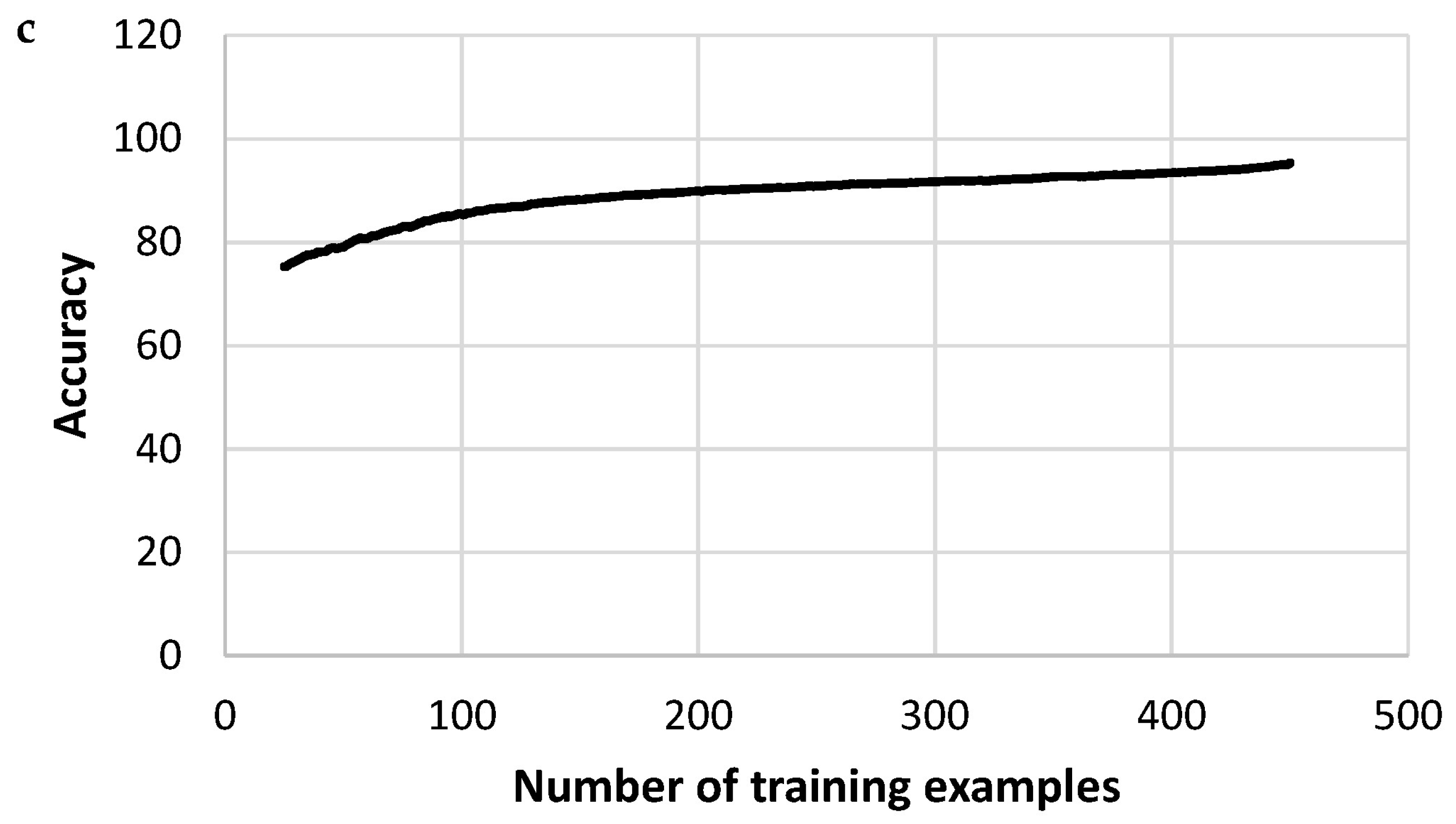
Relative training set size [dimensionless]1.642.052.452.863.273.684.09
Maximal accuracy over the test set [%]67.3374.6784.6784.6784.6789.3394.00
Maximal accuracy over the training set [%]87.6796.0095.5696.8396.1195.0695.33
Number of iterations to achieve maximal accuracy over both sets [iterations]2090120160160220210
Regularization parameter for maximal accuracy10000000
Disclaimer/Publisher’s Note: The statements, opinions and data contained in all publications are solely those of the individual author(s) and contributor(s) and not of MDPI and/or the editor(s). MDPI and/or the editor(s) disclaim responsibility for any injury to people or property resulting from any ideas, methods, instructions or products referred to in the content.

