K-Means Clustering of 51 Geospatial Layers Identified for Use in Continental-Scale Modeling of Outdoor Acoustic Environments

Abstract

Applying machine learning methods to geographic data provides insights into spatial patterns in the data as well as assists in interpreting and describing environments. This paper investigates the results of k-means clustering applied to 51 geospatial layers, selected and scaled for a model of outdoor acoustic environments, in the continental United States. Silhouette and elbow analyses were performed to identify an appropriate number of clusters (eight). Cluster maps are shown and the clusters are described, using correlations between the geospatial layers and clusters to identify distinguishing characteristics for each cluster. A subclustering analysis is presented in which each of the original eight clusters is further divided into two clusters. Because the clustering analysis used geospatial layers relevant to modeling outdoor acoustics, the geospatially distinct environments corresponding to the clusters may aid in characterizing acoustically distinct environments. Therefore, the clustering analysis can guide data collection for the problem of modeling outdoor acoustic environments by identifying poorly sampled regions of the feature space (i.e., clusters which are not well-represented in the training data).

1. Introduction

An important aspect of geographical environments, particularly for land use planning, is sound. In particular, ambient noise, or unwanted outdoor sound due to anthropogenic activity, may negatively affect human and animal life and is therefore important for land use planning. Ambient noise may disrupt sleep, cause hearing loss, increase the risk of cardiovascular disease, and more [1]. For animal species that rely upon sound, competing sounds (e.g., anthropogenic noise) can have varying levels of impact [2], and ambient noise has been indicated as a causal factor for changes in avian behavior and community diversity [3], marine life [4], and anurans (i.e., frogs and toads) [5]. Due to the effects of ambient noise upon both human and animal life, understanding the geographical characteristics of sound is important for urban development and planning, preservation of natural areas (e.g., national parks), and public health.

However, understanding how sound is distributed across, and interacts with, the geographical environment is complex, as abiotic and biotic components of the environment differ in their ability to generate or conduct sound. For example, anthropogenic factors, including urban areas, transportation features/corridors (e.g., railways, airports, etc.), military bases, and energy development operations have all been linked to high levels of ambient noise [6,7] and may also impose additive and potentially interactive effects on overall sound levels. Organisms, on the other hand, may have an ecological effect on shaping and contributing to the acoustic landscape. Many invertebrate and vertebrate species use extensive acoustic displays that periodically influence outdoor sound levels [8,9]. In contrast, vegetation may contribute more to overall outdoor sound levels than animals; not by generating sound, but rather by attenuating or diffusing sound [10].

Geography, geographic data, and geographic techniques have been used in a variety of applications to study both biotic and abiotic components of environments. These applications include using Geographic Information Systems (GIS) to create, store, analyze, and visualize data in a geographic context. GIS lends itself to a variety of domains and aids in interpreting environments. Indeed, GIS has been used by urban land planners to quantify aesthetic values of landscapes [11]. Additionally, GIS has been used in general landscape analysis (e.g., [12]) and to model specific landscape features, such as the visual landscapes in the arid northwest Egypt [11].

Machine learning techniques—both supervised and unsupervised—have been implemented within GIS to map and model various landscape features. Examples of studies which utilize both supervised machine learning and GIS include the use of a decision tree to identify brown bear habitat [13] and the application of four supervised machine learning algorithms (multiple linear regression, support vector machine, artificial neural network, and random forest) to model maize aboveground biomass [14]. Unsupervised machine learning methods on the other hand have been used to study hydrologic catchments in Turkey via k-means clustering [15] and prepare mineral prospectivity maps in central Iran using self-organizing maps and fuzzy c-means [16]. Additionally, supervised and unsupervised machine learning techniques have been used in combination to study urban evolution in Athens, Greece using fuzzy clustering and neural networks [17], classify wetlands in Estonia using k-means clustering and support vector machines [18], and more (e.g., [19,20]).

The ability to adequately study and model ambient sound across large geographic regions is dependent on GIS. Sound mapping is becoming so prevalent in GIS that an open-source sound mapping toolbox has been created for outdoor sound propagation modeling in Esri’s ArcGIS software [21]. Some studies have combined GIS and geographic data with land use regression models to estimate traffic noise [22,23] and overall environmental noise [24]. GIS and supervised machine learning models have also been used over continental scales to predict average outdoor sound levels [25,26]. Further, soundscapes (i.e., the acoustic environment as perceived and evaluated by humans) have been studied using GIS in a variety of outdoor environments [27,28,29,30].

In this paper, we describe a k-means clustering analysis of 51 geospatial layers relevant to outdoor geospatial acoustic modeling in the continental United States (CONUS) [26]. The geospatial layers include descriptors of anthropogenic activity, landscape structure and characteristics, land use, land cover, and climate. K-means clustering was selected, in part, because of its simplicity, efficiency, relatively low computational cost, and common use as a clustering method [31]. Additionally, the application of k-means to our data set produces clear, human-interpretable clusters. Maps of the clustering results as well as correlations between the geospatial layers and clusters are used to identify geospatial characteristics of the different clusters. In particular, we make connections between the clusters and geospatially distinct environments.

This interpretation of the clusters aids in determining acoustically distinct environments. Although the clusters are not tied to specific acoustic characteristics, their distinct geospatial characteristics likely correspond to distinct acoustic environments. Areas corresponding to the same cluster may share acoustic characteristics despite being separated by potentially large physical distances.

We discuss how the clustering results can guide acoustic data collection for the problem of predicting average outdoor sound levels over continental scales using supervised machine learning. We previously used the 51 geospatial features and acoustic training data from 496 unique sites to train a supervised machine learning model to predict outdoor sound levels over the CONUS [26]. In this paper we identify poorly sampled clusters in the training data from which to target future data collection efforts.

2. Materials and Methods

2.1. Geospatial Layers

A set of 51 geospatial raster layers, each with a 270 m spatial resolution, was obtained from the National Park Service Natural Sounds and Night Skies and Inventory and Monitoring Divisions database [32,33]. These layers can be classified into five categories: topography, climate, land cover and land use, hydrology, and anthropogenic. A list of these 51 layers is given in Table 2 of the Supplementary Material for [26], and a more detailed description of each layer is given in Table 1 of the same Supplementary Material. For simplicity, a list of those layers and their descriptions is copied here in Appendix A (

Table A1. CONUS geospatial layers used in clustering, their area of analysis, description and units.

Variable	Area of Analysis	Description	Units
Topography   Elevation   Slope	Point Point	Digital elevation, height above sea level Rate of change in elevation	m degrees
Climate   PPTSummer   PPTWinter   TMaxSummer   TmaxWinter   TminSummer   TminWinter   TdewAvgSummer   TdewAvgWinter	Point Point Point Point Point Point Point Point	10-year average summer precipitation 10-year average winter precipitation 10-year average summer maximum temperature 10-year average winter maximum temperature 10-year average summer minimum temperature 10-year average winter minimum temperature 10-year average summer minimum dew point 10-year average winter maximum dew point	mm mm °C °C °C °C °C °C
Land Cover   Barren   Cultivated   Deciduous   Developed   Evergreen   Herbaceous   Mixed Forest   Shrubland   Water   Wetlands	200 m, 5 km 200 m, 5 km 200 m, 5 km 200 m, 5 km 200 m, 5 km 200 m, 5 km 200 m, 5 km 200 m, 5 km 200 m, 5 km 200 m, 5 km	Proportion of barren land cover Proportion of cultivated land cover Proportion of deciduous forest land cover Proportion of developed land cover Proportion of evergreen forest land cover Proportion of herbaceous land cover Proportion of mixed forest land cover Proportion of shrubland land cover Proportion of water (only) land cover Proportion of wetlands land cover	% % % % % % % % % %
Hydrology   DistCoast   DistStreamO	Point Point	Distance to nearest coastline Distance to nearest stream with Strahler order greater than 1, 3, or 4	m m
Anthropogenic   DistAirpHeli   DistAirpHigh   DistAirpLow   DistAirpMod   DistAirpMoto   DistMilitary   DistRailroads   DistRoadsAll   DistRoadsMaj   FlightFreq   MilitarySum   PopDensity   RddAll   RddMajor   VIIRS	Point Point Point Point Point Point Point Point Point 25 km 40 km Point Point, 5 km Point, 5 km 270 m	Distance to nearest heliport Distance to nearest high-volume airport Distance to nearest low-volume airport Distance to nearest moderate-volume airport Distance to nearest airport (any type) Distance to nearest military flight path Distance to nearest rail line Distance to nearest road (all roads) Distance to nearest road (major roads) Total weekly flight observations Sum of designated military flight paths 2010 Census population density data Road density, sum of road lengths (all roads) divided by area of interest Road density, sum of road lengths (major roads only) divided by area of interest Mean upward radiance at night	m m m m m m m m m count count persons/km2 km/km2 km/km2 nW/cm2/sr

). Note that some variable names in that table correspond to multiple layers due to processing the variable data over different areas or segmenting it based on a given characteristic property (as in the case of the distance to the nearest stream).

Prior to use in clustering, data were scaled to prevent biases in clustering due to variations in the range of values in different layers. In particular, layers that do not vary with distance (from some acoustic source) were scaled using min–max scaling, which scales data to be between zero and one while preserving the shape of the data distribution. For geospatial features that rely on distance (e.g., distance to the nearest coastline or distance to the nearest high-volume airport), an arctangent function was used to scale data to be between zero and one. An arctangent function was applied to distance-dependent features to emphasize changes in distance close to points of interest (e.g., the coast, airports). We note that these 51 features were downselected from a larger set and scaled for the purpose of modeling outdoor sound levels. For further explanation of how the 51 geospatial layers were selected and scaled, we refer the interested reader to [34].

The raw geospatial data occupy about 39 GB of disk space and much of the computation described in this paper was performed on high-memory (128 or 256 GB RAM) nodes on Brigham Young University’s supercomputer.

2.2. Acoustic Data

Acoustic data were collected at 496 unique geographic sites using high-quality sound level meters. Data were collected over a minimum of two to three days, but often closer to two weeks or more, depending on the variability of sound levels at the site, to obtain average values of various acoustic metrics. Our previous work focused on modeling the summer daytime A-weighted L₅₀ over the CONUS [26] (A-weighting is a transformation on the data to account for how the human ear perceives different frequencies, and L₅₀ is the median sound level). Independent of the acoustic metric is the fact that the acoustic training data is limited since we have data at fewer than 500 geographic locations and want to make accurate predictions over the CONUS (See the Supplementary Material for [26] for further information about the acoustic data).

Ideally, we would have a much larger training data set. However, acoustic training data are expensive to collect because of travel costs and time, equipment costs, and the duration of time required to get sufficient data. Therefore, it is necessary to consider which locations are best for future data collection.

2.3. K-Means Clustering

K-means clustering is an unsupervised machine learning algorithm which clusters data into k clusters. More specifically, the algorithm first randomly selects k samples from the data set to initialize the k cluster centroids. Each data point is then assigned to the cluster corresponding to the closest centroid as measured by the Euclidean distance. Centroid locations are then updated to correspond to the mean of all data points in the corresponding cluster. The process of assigning data points to the nearest cluster centroid and adjusting centroid locations is repeated until cluster centroids are stable. Hence, k-means clustering attempts to identify natural clusters in the data [35]. We used k-means clustering as implemented in the Python library scikit-learn [36].

We note that more advanced clustering methods exist, but k-means is a reasonable choice for our dataset. Since data are already custom scaled for modeling outdoor acoustic environments via machine learning, the Euclidean distance is likely a decent indicator of similarity between points in feature space. More sophisticated clustering methods may use different distance measures or rescale data, undermining the effect of scaling the data to describe outdoor acoustic environments.

One challenge of k-means clustering is determining the appropriate number of k clusters such that data are classified meaningfully and descriptively. Two common methods for determining the appropriate number of clusters are silhouette analysis and elbow analysis. Silhouette analysis is performed by calculating the average silhouette score for k-means clustering models trained using various values of k and selecting the model with the highest score. The silhouette score is a measure of how similar points within the same cluster are and how dissimilar points from different clusters are [37]. The silhouette score ranges from –1 to 1, where 1 represents perfectly clustered data and –1 represents poorly clustered data.

Similar to the silhouette analysis, elbow analysis requires training multiple k-means clustering models for different values of k. Elbow analysis uses the inertia (i.e., the sum of squares distance between the data and its nearest cluster) to identify an appropriate number of clusters. The inertia is a monotonic decreasing function, and the optimal number of clusters is the point where adding another cluster to the model begins to only marginally reduce the inertia [38]. This happens at the “elbow” in a plot of the inertia. We used silhouette and elbow analyses to identify the appropriate number of k clusters for a set of 51 geospatial layers over the CONUS.

2.4. Subclustering

To further examine the geospatial data and their clusters, we performed a clustering analysis on each of the initial k clusters. We note that the subclusters identified by this analysis would generally not be identified in the initial clustering analysis, even allowing for different numbers of initial k clusters, because the data considered during clustering are different. During the initial clustering analysis, data from all of the CONUS are used, but during this subclustering analysis, data are separated by their initial clustering assignment. Hence, subclustering identifies natural groupings or clusters within each of the initial clusters, which would not have been apparent in the initial clustering.

Similar to the initial clustering analysis, we had to identify an appropriate number of subclusters for each of the initial clusters. We used silhouette analysis and found that for all clusters, the optimal number of subclusters was determined to be two. Note that the silhouette score cannot be calculated for a single cluster, so silhouette analysis cannot indicate whether a single cluster (i.e., no subclustering) should be preferred.

Therefore, to determine if subclustering into two subclusters is beneficial for any individual cluster, the estimated probability densities of the distance (as measured by the Euclidean norm) between instances within each subcluster and the corresponding initial cluster centroid were plotted. These plots were overlaid with similar plots using the identified subcluster centroids (rather than the initial cluster centroid). This was performed for each cluster to compare the results of subclustering into two subclusters and performing no subclustering. These distributions can be seen in Appendix B, Figure A1, Figure A2, Figure A3, Figure A4, Figure A5, Figure A6, Figure A7 and Figure A8. For the case in which adding a second centroid (i.e., subclustering into two clusters) significantly moved both distributions to the left, it is more likely that subclustering is beneficial for further describing the data. Marginal shifts indicate that subclustering made only minor improvements in accurately clustering the data at the cost of simplicity in the model.

In this paper, we present results of performing subclustering for all clusters into two subclusters, independent of the changes in the distributions of the distance to centroids shown in Figure A1, Figure A2, Figure A3, Figure A4, Figure A5, Figure A6, Figure A7 and Figure A8. Depending on the desired application of clustering results, subclustering may prove useful even when the results of subclustering do not immediately indicate improved clustering. Although we do not discuss which cases of subclustering appear most beneficial, the interested reader is referred to Appendix B for further subclustering results.

3. Results and Discussion

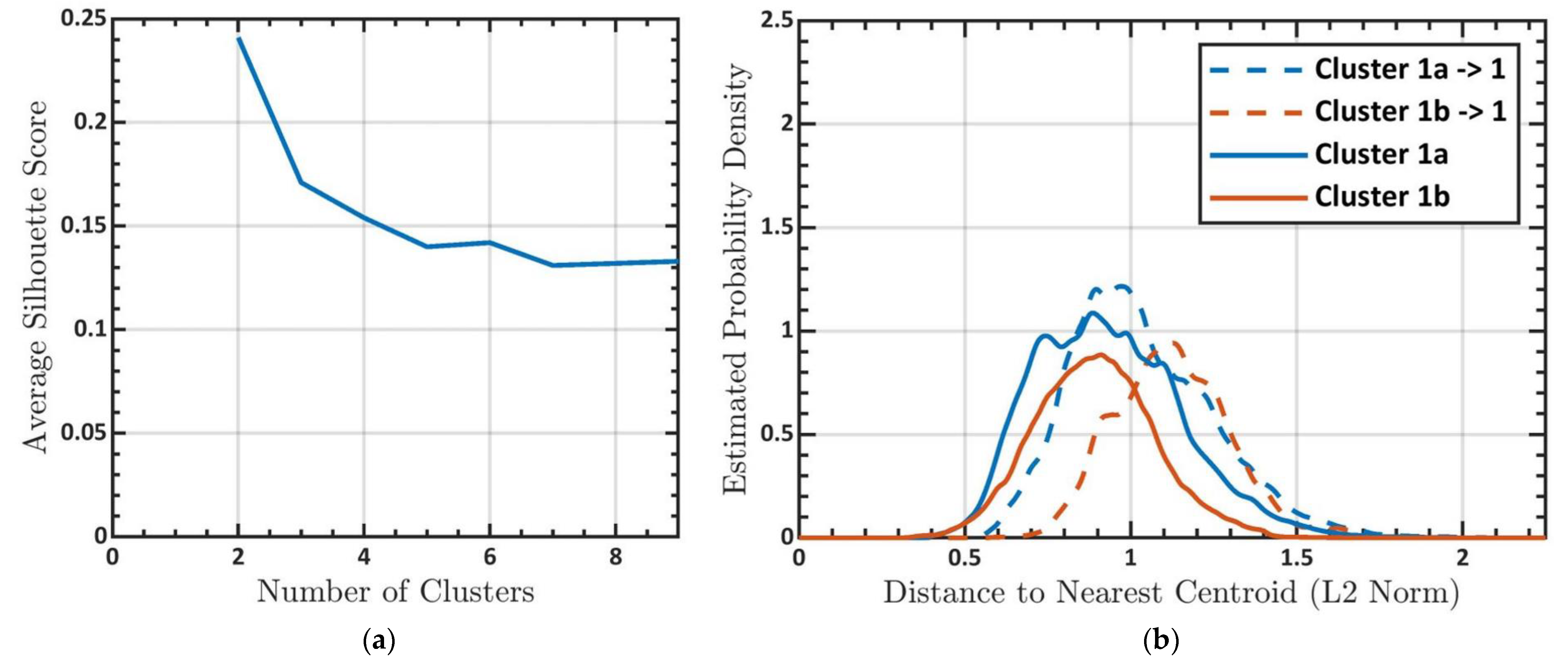
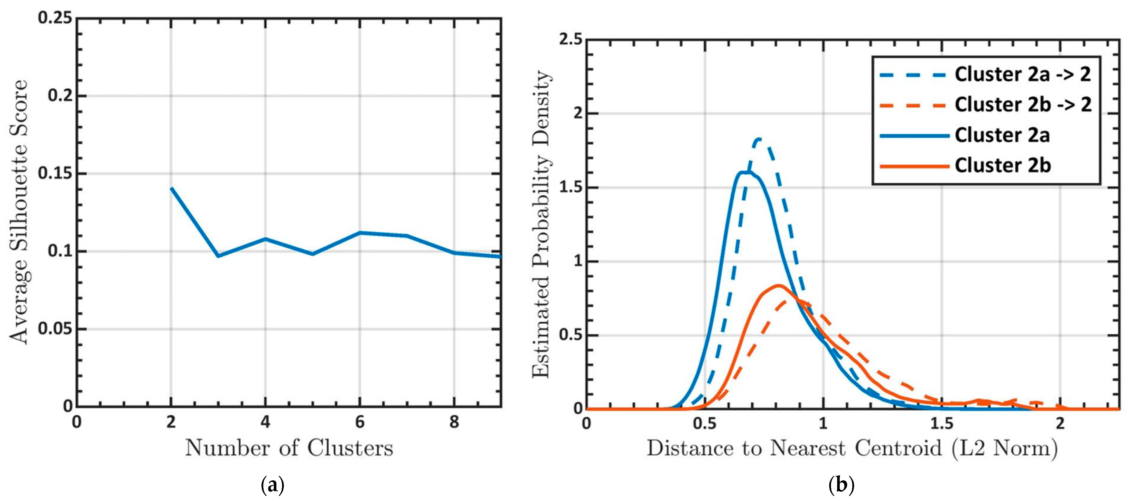
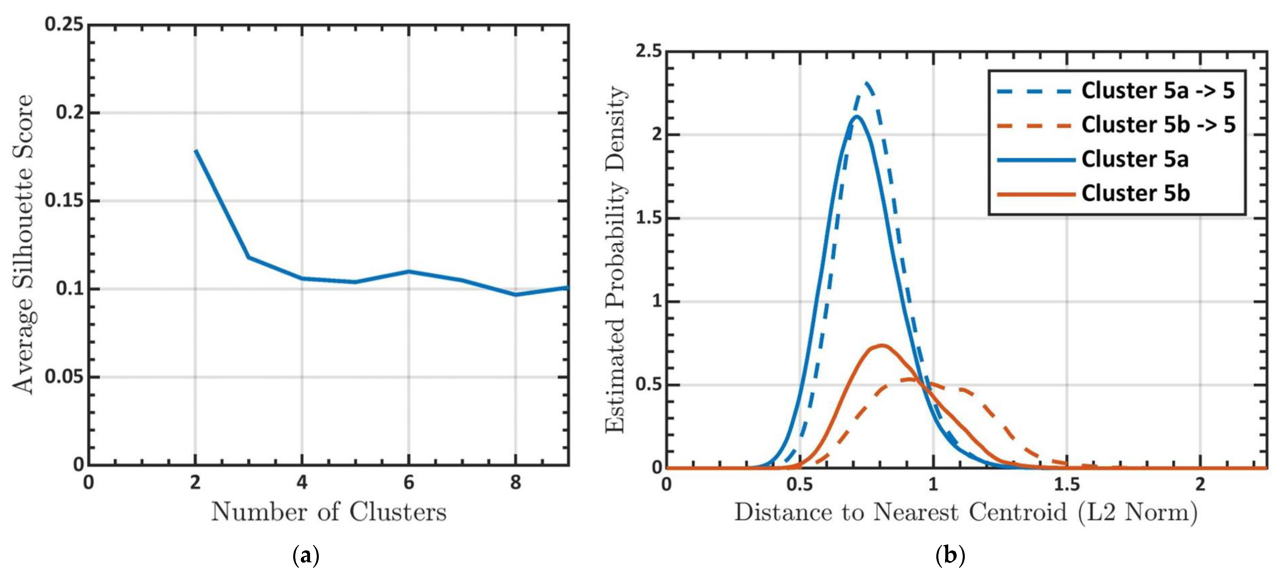
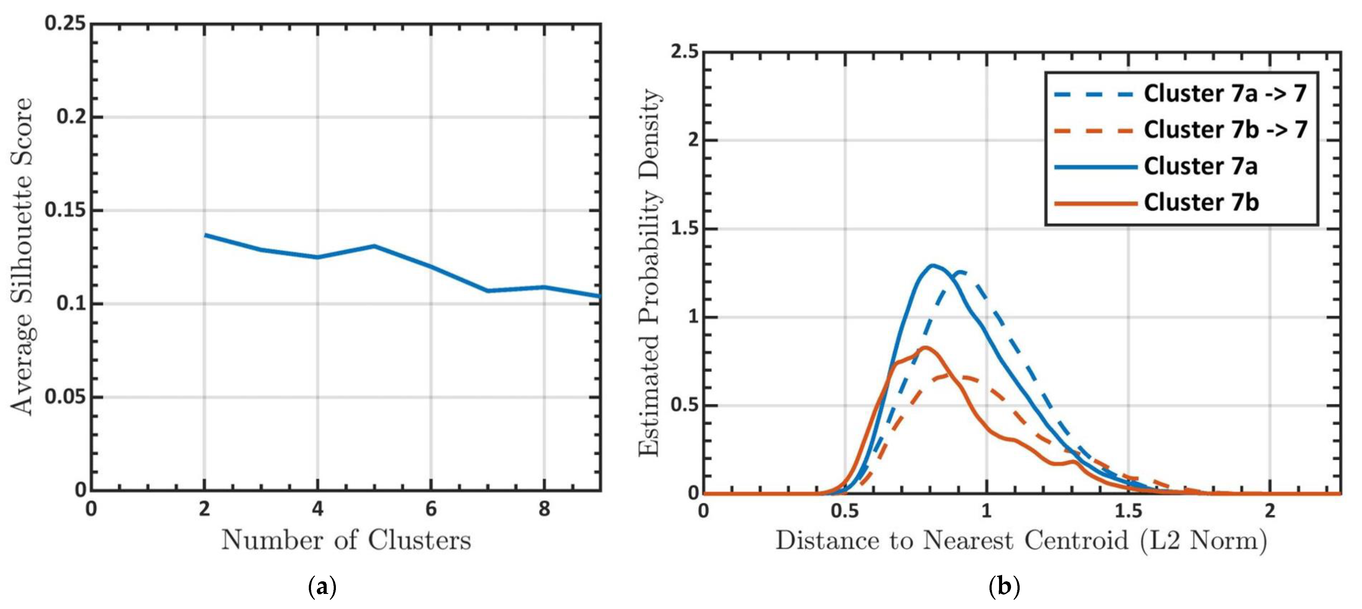
3.1. Determining the Number of Clusters

The results of performing silhouette and elbow analyses on the 51 geospatial layers are shown on the left and right of Figure 1, respectively. Recall that a higher average silhouette score is indicative of better clustering, so the silhouette analysis identifies eight clusters as the optimal number. The results of the elbow analysis are more challenging to interpret because identifying the “elbow” in the plot (i.e., the location at which adding another cluster begins to only marginally reduce the inertia) is somewhat subjective. However, the “elbow” appears to be around seven or nine clusters. Given the subjective nature of determining the location of the “elbow,” we gave more weight to the results of the silhouette analysis. Therefore, we used eight as the optimal number of clusters since both silhouette and elbow analyses indicate this is a reasonable choice. We note that more advanced methods of determining the number of clusters exist [39,40,41] and may be worth exploring in future work.

3.2. Eight-Cluster Model

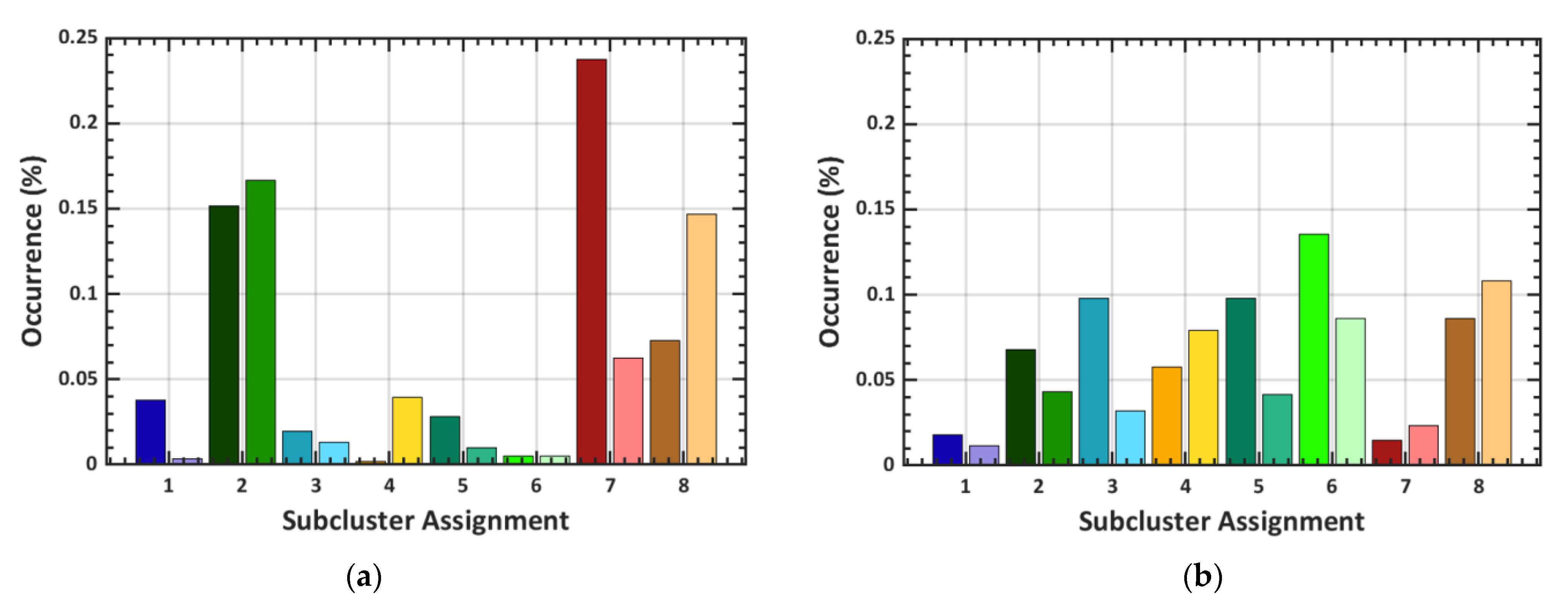
Letting k equal eight, k-means clustering was applied to the 51 geospatial layers for all of the CONUS using a 270-m spatial resolution. Each cluster was assigned a color and a map of the resulting clusters is shown in Figure 2.

To identify geospatial characteristics of the eight clusters, we calculated the correlation between each cluster and the geospatial layers.

Table 1. Top three distinct/unique correlated geospatial variables ranked by magnitude for each cluster.

Cluster Number	Rank 1	Rank 2	Rank 3
1	Water (0.91)	DistCoast (−0.44)	DistRoadsAll (0.35)
2	Evergreen (0.78)	Slope (0.46)	TMinSummer (−0.46)
3	TdewAvgWinter (0.50)	Wetlands (0.49)	TMinWinter (0.42)
4	Herbaceous (0.88)	PPTWinter (−0.28)	DistAirpHigh (0.28)
5	Deciduous (0.84)	MixedForest (0.29)	PPTSummer (0.27)
6	Cultivated (0.89)	Shrubland (−0.32)	DistRailroads (−0.29)
7	Developed (0.76)	RddMajor (0.70)	RddAll (0.67)
8	Shrubland (0.90)	PPTSummer (−0.49)	TdewAvgSummer (−0.44)

shows the top three distinct/unique correlated geospatial variables as ranked by the magnitude of the Pearson correlation coefficient. Correlation coefficients for each cluster were calculated using the scaled geospatial layers and Boolean values to denote whether a site resided within the given cluster. Note that for geospatial variables corresponding to multiple layers due to differing areas of analysis (e.g., barren land cover at 200 m and 5 km areas of analysis), only the largest magnitude correlation among all layers is reported.

From Figure 2 and Table 1, we see that Cluster 1 is strongly correlated with water and is therefore prevalent along the coasts and larger bodies of water e.g., the Great Salt Lake. Cluster 2 represents evergreen forests and areas with higher degrees of slope, such as the Sierra Nevada. Cluster 3 is impacted by winter dew point temperatures and wetlands—thus representing relatively humid areas such as those in the Gulf and Atlantic coastal plains. Herbaceous vegetation and low amounts of winter precipitation are represented in Cluster 4 throughout the northern and southern plains. Cluster 5 correlates with both deciduous and mixed forest environments while Cluster 6, which includes central California and much of the Corn Belt, is most strongly correlated with cultivated (crop) land. Cluster 7 is heavily influenced by developed or urban areas. Finally, Cluster 8 is characteristic of shrubland with low summer precipitation and low summer dew point average, such as the Great Basin Desert.

Seven of the eight clusters’ most impactful variables are land cover-related and five of those seven are strongly correlated with vegetation. This indicates that land cover (especially vegetation) may be the most important factor when differentiating between the clusters. However, other variables, such as dew point temperature and precipitation are also important in determining cluster assignments (Table 1). In particular, the only cluster with a non-land cover variable ranked as the most correlated variable was Cluster 3 (winter dew point average temperature ranked only slightly higher than wetlands land cover).

Viewing zoomed-in maps can allow for further insights and understanding of the clustering model. Figure 3 shows a zoomed-in cluster map of the Great Lakes region and Northeast. The upper Midwest and northeastern United States are dominated by Clusters 5, 6, and 7. Cluster 5 is heavily impacted by deciduous forest and Cluster 6 is mostly influenced by cultivated (crop) land. The large urban/suburban areas of Chicago, Detroit, Minneapolis, Boston, New York City, etc. are in Cluster 7, which is most strongly affected by developed land cover. Additionally, Cluster 1 dominates coastlines both to the ocean and along the Great Lakes, as well as lakes.

Figure 4 (left) shows a zoomed-in cluster map of Utah. The west/southwest region of the United States (including Utah) is primarily represented by Clusters 8 and 2, which are most strongly correlated with shrubland and evergreen land cover, respectively. Indeed, we see many mountainous forested regions of Utah (e.g., High Uinta Wilderness) grouped into Cluster 2 and flatter desert-like areas (e.g., the Sevier Desert) grouped into Cluster 8. Interestingly, the Great Salt Lake Desert in northwestern Utah is assigned to Cluster 2, despite not containing evergreen trees or having significant slope. However, the Great Salt Lake Desert is a unique region and likely has the most similarities with the climate typical of Cluster 2. In Utah, both the Great Salt Lake and Utah Lake are assigned to Cluster 1, while the most populated cities (e.g., Salt Lake City, Ogden, and Provo) are assigned to Cluster 7. All eight clusters are present in Utah, possibly indicating a wider variety of environments than in many other states.

Figure 4 (right) shows a zoomed-in cluster map of the eastern/southeastern coastal plains, much of which are represented by Cluster 3, which is positively correlated with average winter dew point temperatures and wetlands. Deciduous forests are evident in Cluster 5 throughout much of the Piedmont and Appalachian Mountains. The coastline, bays, rivers, and lakes are grouped into Cluster 1, while urban/suburban areas are well-mapped in Cluster 7. In particular, the developed northern Virginia–Washington DC–Baltimore–Philadelphia corridor is striking.

As apparent with Clusters 6 and 7, anthropogenic features (e.g., cultivation and urban land development) play a role in landscape-level clusters. However, the way in which anthropogenic features influence clustering varies across spatial scales. For example, urban and suburban areas (Cluster 7) demonstrate a concentrated effect on the clusters, whereas cultivated areas and railroads (Cluster 6) have a much broader effect on clusters that occur over large expanses (e.g., much of the Midwest). Humans have an influential role on ecosystems, and it is not surprising that anthropogenic features may impose additive effects on the clusters across landscapes.

3.3. Subclustering

Each of the initial eight clusters was further divided into two subclusters. We refer to the first and second subcluster for each cluster by the corresponding cluster number and a letter, “a” for the first subcluster and “b” for the second subcluster. For example, Subclusters 8a and 8b are the subclusters corresponding to Cluster 8 (colored brown in maps above). For simplicity, we will refer to the model which subclusters each of the original eight clusters into two subclusters as the 16-subcluster model. A CONUS map of the subclusters is given in Figure 5 (see Figure A9 for individual CONUS subcluster maps). The first color for each subcluster, corresponding to all “a” subclusters, is the same as the initial cluster color. The second color for each subcluster, corresponding to all “b” subclusters, is a lighter shade of each initial cluster color.

The 8-cluster and 16-subcluster models are overall similar in identifying influential environmental factors underlying the model cluster assignments (see Table 1 and

Table 2. Top three distinct/unique correlated geospatial variables ranked by magnitude for each subcluster.

Subcluster Number	Rank 1	Rank 2	Rank 3
1a	Water (0.70)	DistCoast (−0.58)	DistRoadsAll (0.34)
1b	Water (0.60)	DistRoadsAll (0.14)	TMaxWinter (−0.08)
2a	Evergreen (0.78)	Slope (0.38)	TMinSummer (−0.34)
2b	Elevation (0.31)	Evergreen (0.30)	TMinSummer (−0.29)
3a	TdewAvgWinter (0.43)	TMaxWinter (0.37)	TMinWinter (0.37)
3b	Wetlands (0.79)	PPTSummer (0.27)	TdewAvgWinter (0.23)
4a	Herbaceous (0.57)	DistMilitary (−0.18)	TMaxSummer (0.15)
4b	Herbaceous (0.63)	DistAirpHigh (0.31)	TMinWinter (−0.27)
5a	Deciduous (0.78)	PPTSummer (0.25)	FlightFreq_25km (0.25)
5b	MixedForest (0.39)	Deciduous (0.29)	TMaxWinter (−0.27)
6a	Cultivated (0.65)	DistAirpHeli (−0.28)	Elevation (−0.27)
6b	Cultivated (0.53)	TMinWinter (−0.31)	TMaxWinter (−0.27)
7a	Developed (0.44)	RddAll (0.31)	RddMajor (0.30)
7b	RddMajor (0.74)	Developed (0.74)	RddAll (0.67)
8a	Shrubland (0.59)	TMaxSummer (0.41)	TMaxWinter (0.36)
8b	Shrubland (0.62)	TdewAvgSummer (−0.48)	Elevation (0.45)

). Rankings in Table 2 were calculated in a similar manner to those in Table 1. Some of the largest observable differences between the 8-cluster and 16-subcluster models are the further distinction of Clusters 3, 7, and 8. In the 16-subcluster model, predominant wetland areas within Cluster 3 are more clearly separated from the rest of the coastal plains. Subclustering also helps differentiate between two densities of urban activity (Subclusters 7a and 7b). In the 8-cluster model, the deserts of the western United States are represented well by Cluster 8. In the 16-subcluster model however, Cluster 8 subclusters distinguish between the cold (Subcluster 8b) and hot (Subcluster 8a) deserts of the western United States.

3.4. General Applications

The 51 geospatial layers used for the above clustering analysis have previously been used to predict sound levels across the CONUS and were selected because of their potential relationship with outdoor sound levels [26]. These layers are therefore potentially relevant to geospatial acoustic modeling and, more broadly, characterizing acoustic environments. The k-means clustering analysis above attempted to identify geospatially distinct clusters with unique characteristics from the 51 layers. Because these layers may be useful in characterizing acoustic environments, it is not unreasonable to suppose that the clusters may also correspond to acoustically distinct environments. In general, the clusters correlate most strongly with the type of land cover, and different types of land cover likely correspond to different acoustic sources and propagation effects (i.e., distinct acoustic environments).

Characterizing distinct acoustic environments has potential applications in land use planning, both in anthropogenic and natural environments. Of particular interest are acoustic environments corresponding to large amounts of anthropogenic noise, since ambient noise often results in much higher sound pressure levels and can have harmful effects on human health [42] and wildlife [2]. Identifying acoustic environments with high/low amounts of anthropogenic noise is valuable in urban planning, public health, and wildlife policy and management (including identifying suitable wildlife corridors). More broadly, characterizing distinct acoustic environments is important to understanding and classifying different geographic locations, as well as finding commonalities between regions independent of physical distance.

3.5. Limitations of General Applications

The 51 geospatial layers were selected and scaled with the goal of distinguishing different acoustic environments [26]. However, it is likely that there are acoustic sources and propagation effects which are not well-represented in the geospatial data. Additionally, it is possible that some acoustic effects are not well-represented in clusters due to trends in a larger number of geospatial layers, which dominate clustering assignments. We also note that the spatial resolution (270 m) makes cluster maps ineffective at investigating local (i.e., over small spatial regions; e.g., <1 km) cluster assignments or patterns.

3.6. Application to Outdoor Sound Level Modeling

Because the clusters may represent different acoustic environments, they can help identify which locations should be targeted for future acoustic data collection. Figure 6 shows the distribution of clusters in the training data (a) and the CONUS (b). We see that these distributions are quite different, with Cluster 7 (especially Subcluster 7a) being the most overrepresented and Cluster 6 being the most underrepresented.

Recall that Cluster 7 is characterized by developed land cover and high road density and is therefore likely one of the most complex acoustic environments. Additionally, ambient noise is likely large within Cluster 7, making accurate predictions of sound levels within this cluster of greater importance for public health. Therefore, it is reasonable to sample this cluster more heavily than many of the others for human-focused applications.

Cluster 6, on the other hand, which is generally characterized by cultivated (crop) land, is the most common cluster in the CONUS and the least common cluster (after combining data from both subclusters) in the training data. This indicates that we should target future data collection efforts in Cluster 6 first to improve overall model performance in the CONUS.

4. Conclusions

We applied k-means clustering to a set of 51 geospatial layers, selected because of their relevance to geospatial acoustic modeling in the continental United States, and custom-scaled for such models [26]. The resulting 8-cluster model identified eight geospatially distinct regions in the continental United States, which differ by land cover, vegetation, anthropogenic activity, climate, etc. Land cover and largescale patterns of vegetation are influential in the clustering, with seven of the eight clusters most strongly correlated with a distinct type of land cover, five of which are vegetation communities. Importantly, each cluster corresponds to a different type of land cover and/or climate.

Because the 51 geospatial layers used in clustering are relevant to geospatial acoustic modeling, the geospatially distinct environments corresponding to each cluster may aid in determining acoustically distinct environments. Indeed, it is reasonable to suppose that differences in land cover, climate, anthropogenic activity, etc. likely result in different acoustic sources and propagation effects (i.e., different acoustic environments). Characterizing acoustic environments has potential applications in land use planning (e.g., urban planning and wildlife policy and management). More broadly, characterization of acoustic environments is an important aspect of describing and classifying geospatial environments and landscapes. These results can be applied to continental-scale modeling of outdoor acoustic environments by identifying underrepresented clusters in the training data set for targeted data collection.

K-means clustering was implemented in this study, in part, because of its simplicity, interpretability, and low computational costs. These characteristics are all desirable in data analysis, and k-means is available in multiple coding, software, and platform settings. Further, k-means is one of the most used clustering algorithms in data analysis [31] and produces human-interpretable clusters on our data set, which can help characterize acoustic environments and direct data collection efforts for continental-scale models of outdoor sound levels. There may be value in exploring additional clustering algorithms, such as DBSCAN, Gaussian mixture models, and mean-shift clustering, or more advanced methods of determining the number of clusters [39,40,41]. However, none of these are computationally trivial given the size of the dataset, and the results of k-means clustering (and subclustering) provide sufficient information to guide current acoustic data collection methods. Therefore, future research will focus on applying these clustering results for targeted data collection for improving continental-scale models of outdoor sound levels.

References

1. Fink, D. Ambient Noise Is “The New Secondhand Smoke”. Acoust. Today 2019, 15, 38–46. [Google Scholar] [CrossRef]
2. Kight, C.R.; Swaddle, J.P. How and why environmental noise impacts animals: An integrative, mechanistic review. Ecol. Lett. 2011, 14, 1052–1061. [Google Scholar] [CrossRef] [PubMed]
3. Francis, C.D.; Ortega, C.P.; Cruz, A. Noise pollution changes avian communities and species interactions. Curr. Biol. 2009, 19, 1415–1419. [Google Scholar] [CrossRef] [PubMed] [Green Version]
4. Rako-Gospić, N.; Picciulin, M. Underwater noise: Sources and effects on marine life. In World Seas: An Environmental Evaluation, 2nd ed.; Sheppard, C., Ed.; Academic Press: Cambridge, MA, USA, 2019; Volume 3, pp. 367–389. [Google Scholar] [CrossRef]
5. Sun, J.W.; Narins, P.M. Anthropogenic sounds differentially affect amphibian call rate. Biol. Conserv. 2005, 121, 419–427. [Google Scholar] [CrossRef]
6. Buxton, R.T.; McKenna, M.F.; Mennitt, D.; Brown, E.; Fristrup, K.; Crooks, K.R.; Angeloni, L.M.; Wittemyer, G. Anthropogenic noise in US national parks–sources and spatial extent. Front. Ecol. Environ. 2019, 17, 559–564. [Google Scholar] [CrossRef]
7. Jones, N.F.; Pejchar, L.; Kiesecker, J.M. The Energy Footprint: How Oil, Natural Gas, and Wind Energy Affect Land for Biodiversity and the Flow of Ecosystem Services. BioScience 2015, 65, 290–301. [Google Scholar] [CrossRef] [Green Version]
8. Sueur, J. Cicada acoustic communication: Potential sound partitioning in a multispecies community from Mexico (Hemiptera: Cicadomorpha: Cicadidae). Biol. J. Linn. Soc. 2002, 75, 379–394. [Google Scholar] [CrossRef]
9. Berg, K.S.; Brumfield, R.T.; Apanius, V. Phylogenetic and ecological determinants of the neotropical dawn chorus. Proc. R. Soc. Ser. B Biol. Sci. 2006, 273, 999–1005. [Google Scholar] [CrossRef]
10. Aylor, D. Noise reduction by vegetation and ground. J. Acoust. Soc. Am. 1972, 51, 197–205. [Google Scholar] [CrossRef]
11. Ayad, Y.M. Remote Sensing and GIS in modeling visual landscape change: A case study of the northwestern arid coast of Egypt. Landscape Urban Plann. 2005, 73, 307–325. [Google Scholar] [CrossRef]
12. Statuto, D.; Cillis, G.; Picuno, P. GIS-based Analysis of Temporal Evolution of Rural Landscape: A Case Study in Southern Italy. Nat. Resour. Res. 2019, 28, S61–S75. [Google Scholar] [CrossRef]
13. Kobler, A.; Adamic, M. Identifying brown bear habitat by a combined GIS and machine learning method. Ecol. Modell. 2000, 135, 291–300. [Google Scholar] [CrossRef]
14. Han, L.; Yang, G.; Dai, H.; Xu, B.; Yang, H.; Feng, H.; Li, Z.; Yang, X. Modeling maize above-ground biomass based on machine learning approaches using UAV remote-sensing data. Plant Methods 2019, 15, 10. [Google Scholar] [CrossRef] [PubMed] [Green Version]
15. Aytaç, E. Unsupervised learning approach in defining the similarity of catchments: Hydrological response unit based k-means clustering, a demonstration on Western Black Sea Region of Turkey. Int. Soil Water Conserv. Res. 2020, 8, 321–331. [Google Scholar] [CrossRef]
16. Abedi, M.; Norouzi, G.H.; Torabi, S.A. Clustering of mineral prospectivity area as an unsupervised classification approach to explore copper deposit. Arabian J. Geosci. 2013, 6, 3601–3613. [Google Scholar] [CrossRef]
17. Grekousis, G.; Manetos, P.; Photis, Y.N. Modeling urban evolution using neural networks, fuzzy logic and GIS: The case of the Athens Metropolitan area. Cities 2013, 20, 193–203. [Google Scholar] [CrossRef]
18. Ahmed, K.R.; Akter, S.; Marandi, A.; Schüth, C. A simple and robust wetland classification approach by using optical indices, unsupervised and supervised machine learning algorithms. Remote Sens. Appl. Soc. Environ. 2021, 23, 100569. [Google Scholar] [CrossRef]
19. Chang, Z.; Du, Z.; Zhang, F.; Huang, F.; Chen, J.; Li, W.; Guo, Z. Landslide susceptibility prediction based on remote sensing images and GIS: Comparisons of supervised and unsupervised machine learning models. Remote Sens. 2020, 12, 502. [Google Scholar] [CrossRef] [Green Version]
20. Rozenstein, O.; Karnieli, A. Comparison of methods for land-use classification incorporating remote sensing and GIS inputs. Appl. Geogr. 2011, 31, 533–544. [Google Scholar] [CrossRef]
21. Keyel, A.C.; Reed, S.E.; McKenna, M.F.; Wittemyer, G. Modeling anthropogenic noise propagation using the Sound Mapping Tools ArcGIS toolbox. Environ. Model. Softw. 2017, 97, 56–60. [Google Scholar] [CrossRef]
22. Aguilera, I.; Foraster, M.; Basagaña, X.; Corradi, E.; Deltell, A.; Morelli, X.; Phuleria, H.C.; Ragettli, M.S.; Rivera, M.; Thomasson, A.; et al. Application of land use regression modelling to assess the spatial distribution of road traffic noise in three European cities. J. Exposure Sci. Environ. Epidemiol. 2015, 25, 97–105. [Google Scholar] [CrossRef]
23. Chang, T.Y.; Liang, C.H.; Wu, C.F.; Chang, L.T. Application of land-use regression models to estimate sound pressure levels and frequency components of road traffic noise in Taichung, Taiwan. Environ. Int. 2019, 131, 104959. [Google Scholar] [CrossRef]
24. Xie, D.; Liu, Y.; Chen, J. Mapping Urban Environmental Noise: A Land Use Regression Method. Environ. Sci. Technol. 2011, 45, 7358–7364. [Google Scholar] [CrossRef]
25. Mennitt, D.J.; Fristrup, K.M. Influence factors and spatiotemporal patterns of environmental sound levels in the contiguous United States. Noise Control Eng. J. 2016, 64, 342–353. [Google Scholar] [CrossRef]
26. Pedersen, K.; Transtrum, M.K.; Gee, K.L.; Lympany, S.V.; James, M.M.; Salton, A.R. Validating two geospatial models of continental-scale environmental sound levels. JASA Express Lett. 2021, 1, 122401. [Google Scholar] [CrossRef] [PubMed]
27. Eve, S. The embodied GIS. Using Mixed Reality to explore multi-sensory archaeological landscapes. Internet Archaeol. 2017, 44. [Google Scholar] [CrossRef]
28. Primeau, K.E.; Witt, D.E. Soundscapes in the past: Investigating sound at the landscape level. J. Archaeol. Sci. Rep. 2018, 19, 875–885. [Google Scholar] [CrossRef]
29. Hong, J.Y.; Jeon, J.Y. Soundscape mapping in urban contexts using GIS techniques. Inter-Noise 2014. [Google Scholar]
30. Youssoufi, S.; Houot, H.; Viudel, G.; Pujol, S.; Mauny, F.; Foltete, J.-C. Combining visual and noise characteristics of a neighborhood environment to model residential satisfactions: An application of GIS-based metrics. Landsc. Urban Plan. 2020, 204, 103932. [Google Scholar] [CrossRef]
31. Sinaga, K.P.; Yang, M.-S. Unsupervised K-Means Clustering Algorithm. IEEE Access 2020, 8, 80716–80727. [Google Scholar] [CrossRef]
32. DataStore—Geospatial Sound Modeling. Available online: https://irma.nps.gov/DataStore/Reference/Profile/2217356 (accessed on 3 June 2020).
33. Nelson, L.; Kinseth, M.; Flowe, T. Explanatory Variable Generation for Geospatial Sound Modeling–Standard Operating Procedure. Natural Resource Report NPS/NRSS/NRR–2015/936. National Park Service, Fort Collins, Colorado. 2015. Available online: https://irma.nps.gov/App/Reference/Profile/2221202 (accessed on 3 June 2020).
34. Pedersen, K.; Transtrum, M.K.; Gee, K.L.; Lympany, S.V.; James, M.J.; Salton, A.R. Feature Selection for a Continental-Scale Geospatial Model of Environmental Sound Levels. In Review.
35. Xu, R.; Wunsch, D. Survey of clustering algorithms. IEEE Trans. Neural Netw. 2005, 16, 645–678. [Google Scholar] [CrossRef] [PubMed] [Green Version]
36. Pedregosa, F.; Varoquaux, G.; Gramfort, A.; Michel, V.; Thirion, B.; Grisel, O.; Blondel, M.; Prettenhofer, P.; Weiss, R.; Dubourg, V.; et al. Scikit-learn: Machine Learning in Python. J. Mach. Learn. Res. 2011, 12, 2825–2830. [Google Scholar]
37. Rousseeuw, P.J. Silhouettes: A graphical aid to the interpretation and validation of cluster analysis. J. Comput. Appl. Math. 1987, 20, 53–65. [Google Scholar] [CrossRef] [Green Version]
38. Bholowalia, P.; Kumar, A. EBK-Means: A Clustering Technique based on Elbow Method and K-Means in WSN. Int. J. Comput. Appl. 2014, 105, 17–24. [Google Scholar]
39. Sun, J.; Li, Z.; Zou, F.; Yang, Y. Adaptive Determining for Optimal Cluster Number of K-Means Clustering Algorithm. In Proceedings of the 2012 International Conference on Information Technology and Software Engineering: Information Technology & Computing Intelligence, Beijing, China, 8–10 December 2012; pp. 551–560. [Google Scholar] [CrossRef]
40. Huan, D.; Nguyen, D.T. An adaptive method to determine the number of clusters in clustering process. In Proceedings of the 2014 International Conference on Computer and Information Sciences (ICCOINS), Kuala Lumpur, Malaysia, 3–5 June 2014; pp. 1–6. [Google Scholar] [CrossRef]
41. Patil, C.; Baidari, I. Estimating the Optimal Number of Clusters k in a Dataset Using Data Depth. Data Sci. Eng. 2019, 4, 132–140. [Google Scholar] [CrossRef] [Green Version]
42. Moudon, A.V. Real Noise from the Urban Environment: How Ambient Community Noise Affects Health and What Can Be Done About It. Am. J. Prev. Med. 2009, 37, 167–171. [Google Scholar] [CrossRef]
Figure 1. Silhouette (left) and elbow (right) analyses showing the average silhouette score and average inertia, respectively, as the number of clusters is varied.
Applsci 13 08123 g001
Figure 2. Continental United States (CONUS) cluster assignments after clustering 51 geospatial features with a 270-m spatial resolution.
Applsci 13 08123 g002
Figure 3. Cluster assignments in the Great Lakes region and Northeast as a result of clustering 51 geospatial features with a 270-m spatial resolution.
Applsci 13 08123 g003
Figure 4. Cluster assignments in Utah (left) and along the eastern/southeastern coastal plains (right) as a result of clustering 51 geospatial features with a 270-m spatial resolution.
Applsci 13 08123 g004
Figure 5. CONUS subcluster assignments after clustering each cluster from the 8-cluster model into two subclusters.
Applsci 13 08123 g005
Figure 6. Distribution of subclusters within (a) the training data and (b) the CONUS.
Applsci 13 08123 g006