The Behavior of Nonlinear Tsunami Waves Running on the Shelf

Abstract

The problem of creating methods for calculating tsunami parameters and predicting these dangerous events is currently being solved by integrating the equations of the theory of water waves. Both numerical methods and powerful computers are used, as well as analytical solutions. The essential stage is the stage of the tsunami reaching the shelf and shallow coastal waters. The tsunami amplitude increases here, and nonlinear effects become important. Nonlinearity excludes the solution’s unicity and the superposition principle’s fulfillment. The nonlinear theory can have many solutions, depending on various external conditions; there could be nontrivial ones. In this article, we explore the properties of several nonlinear solutions. With their help, we can find the maximum possible amplitude of tsunami waves when approaching the coast and estimate the seismological parameters of an earthquake-generating tsunami.

1. Introduction

Arsen’yev and Eppelbaum [1] gave the following definition: “Tsunamis are long gravity waves in the ocean occurring because of a short-term change in its volume due to large-scale disturbances in the ocean’s surface, shores, or bottom” [2,3,4,5]. Typical tsunami wave periods are from 1 min to several hours, and the characteristic wavelengths are from 100 m to 100 km. Therefore, when approaching the shelf, tsunami waves can nonlinearly interact with the ocean tide’s shallow components, weakening or strengthening the tsunami wave e.g., [1,6].

Tsunamis are a natural disaster that have been intensively studied since the second half of the 20th century. The sources of tsunamis in the oceans and seas are usually earthquakes. However, there may be other reasons: collapses and landslides, the fall of large massifs of rocks into the water, volcanic eruptions, the impact of meteorological disturbances on the ocean, the fall of celestial bodies, powerful underwater explosions (for example, hydrogen bombs), and others. All these natural disasters are described by nonlinear equations e.g., [7,8,9,10,11,12,13,14]. Since tsunami waves often accompany earthquakes, the seismic hazard assessment should also include an assessment of the tsunami hazard. This depends on the amplitude of tsunami waves, which can reach several tens of meters and produce great destruction.

High tsunami waves look like secluded waves, sometimes called solitons [15,16,17,18,19]. They cause the water level to rise, tear ships off their anchors and push them, flood islands, and initiate chaos on the shelf. Tsunami waves can enter bays and harbors, which capture them and excite their vibrations in the form of standing waves (seiches). They can get into resonance with a tsunami, causing the effect of the impact of a tsunami on the shelf to increase significantly [20,21]. Sometimes, tsunamis move in a phase in which the water level ahead is lowered. Such waves are called N-waves [22,23].

Secluded waves were discovered by the English engineer J.S. Russel in 1834. He measured the wave resistance of barges moving in channels [18]. The linear theory of water waves was developed in the first half of the 19th century by Cauchy and Poisson [15,16]. It was based on the equations of a heavy, nonviscous (ideal) fluid in the Earth’s gravitational field. This theory is still used in studying tsunamis near sources [4]. The corresponding models are called nonhydrostatic since they allow large vertical velocities and do not obey the hydrostatic equation. Additional consideration of nonlinearity in the equations of hydrodynamics allowed Boussinesq, Rayleigh, Korteveg, and de Vries to construct a theory of solitary waves [17,18,24,25]. This is used to examine tsunami waves [15,16,19] but needs to consider turbulent friction, which becomes essential during tsunami propagation along the shelf and coastal regions.

The problems of periodic, surface-gravity waves propagating in one horizontal dimension on the water of variable depth were considered by Rajan et al. [26]. Benilov et al. [27] and Grimshaw and Annenkov [28] analyzed nonlinear packets of surface gravity waves over rugged topography governed by a nonlinear Schrödinger equation with variable coefficients.

The effect of dissipation on low-amplitude gravitational-capillary waves was considered in [29]. However, waves of large amplitudes, such as tsunamis running along the shelf, are conveniently studied using hydrodynamic equations integrated over the vertical. One theory shows that eliminating the vertical velocities and using the hydrostatic equation is possible in this case. Therefore, these models are called hydrostatic models or shallow water theory models.

In this paper, we study the nonlinear equations of the shallow water theory and find new solutions that describe solitary tsunami waves traveling along the shelf. It should be noted that these solutions differ from Russell solitons, which arise in an ideal fluid without friction due to the balance of nonlinearity and dispersion typical for waves on water of tremendous or medium depth. There is no dispersion in shallow water; solitary waves can exist here with a balance of nonlinearity and energy dissipation due to friction. These waves can be called dissipative solitons; they also arise, for example, when studying storm surges in oceans and seas [30].

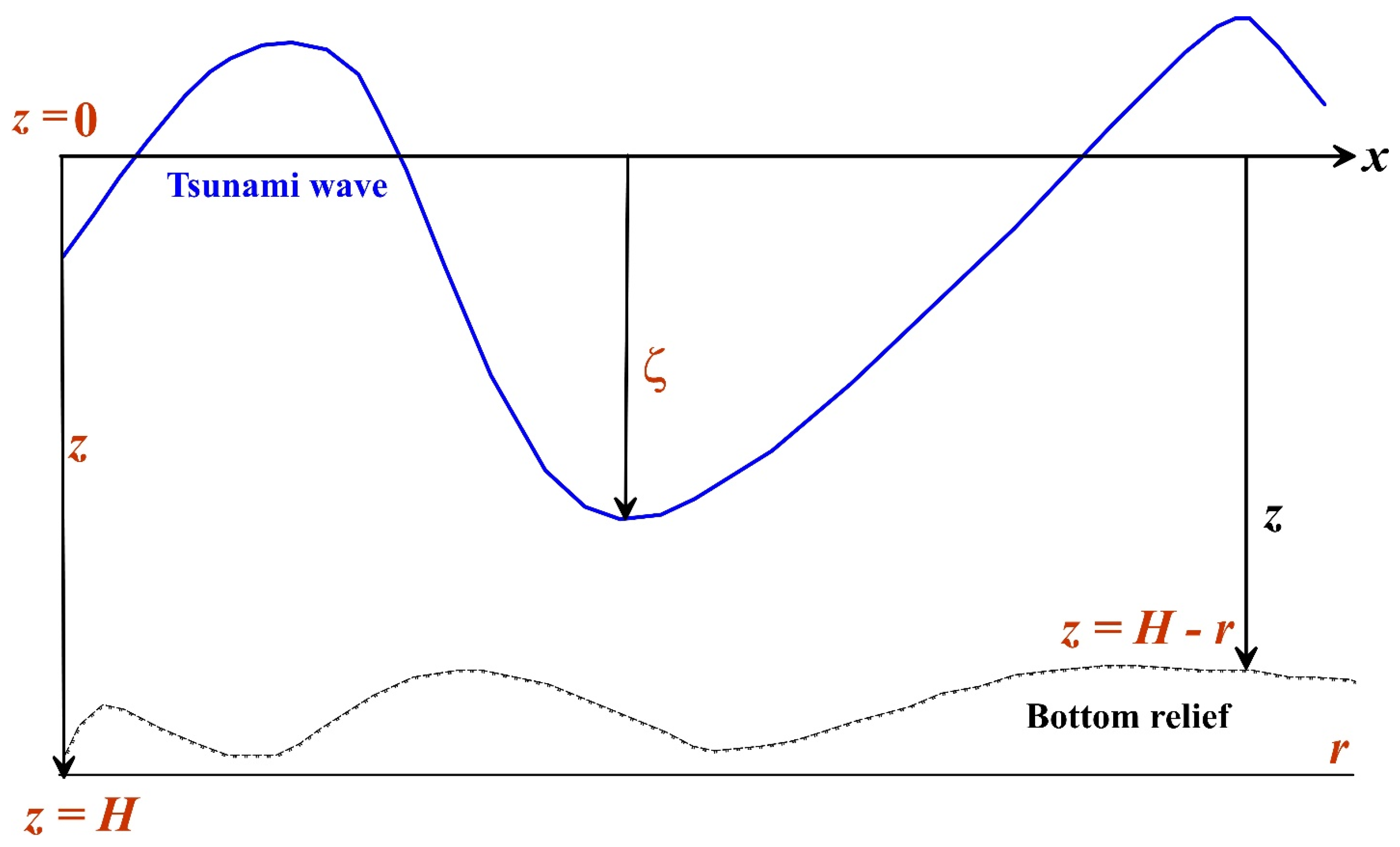
2. Formulation of the Problem

We chose the coordinates’ origin at the shelf’s sea edge x = 0. We directed the x-axis along the direction of wave propagation perpendicular to the coast, the y-axis as perpendicular to the x-axis (left), and the z-axis as vertically down (Figure 1 and Figure 2). The letter M denotes the width of the shelf. The level z = 0 is located on the surface of calm water; the letter z denotes the wave disturbance of the sea surface; the positive value z is counted down from the undisturbed level z = 0 (Figure 2). The letter H denotes the average shelf depth (effects of variable depth and wave refraction are not considered here), and the letter r denotes the average height of the rough protrusions on the bottom so that the total depth of the shelf is H − r.

We used the shallow water theory equations. They are obtained from geophysical hydrodynamic equations by integrating along the z-axis in the range from z = ζ to z = (H − r) [4,31,32]. Assuming that there are no changes along the y-axis (∂/ = 0), we write these equations in the following form:

$$\frac{\partial \varsigma }{\partial t}+\frac{\partial S}{\partial x}\hspace{0.33em}=0,$$

(1)

$$\frac{\partial S}{\partial t}+n\frac{\partial S^2}{\partial x}\hspace{0.33em}=\hspace{0.33em}{c}_0^2\frac{\partial \varsigma }{\partial x}+A_L\frac{{\partial }^{2}S}{\partial x^2}-R_x^H\hspace{0.33em}.$$

(2)

Here, ζ is the perturbation of the water surface level, n = 1/(H − r), c₀² = g (H − r), A_L is the coefficient of horizontal turbulent viscosity, and g is the gravity acceleration. The turbulent friction on the bottom R_x^H can be related to the total flow rate S by a linear law:

$$R_x^H={\omega }_{T}S,\hspace{0.33em}{\omega }_T=\frac{3A}{{\left(H-r\right)}^2},S={\int }_{\varsigma }^{H-r}udz\hspace{0.33em}.$$

(3)

Here, ω_T is the relaxation frequency (friction), A is the coefficient of vertical turbulent viscosity [33], and u is the flow velocity component in the wave along the x-axis. We also consider another nonlinear friction law below at the end of this article.

Equation (2) can be conveniently reduced to the dimensionless form:

$$\frac{{\partial }^2\Pi }{\partial T^2}\hspace{0.33em}+Fr\frac{{\partial }^2{\Pi }^2}{\partial T\partial X}+F_B\frac{\partial \Pi }{\partial T}\hspace{0.33em}-F_L\frac{{\partial }^3\Pi }{\partial T\partial X^2}-\frac{{\partial }^2\Pi }{\partial X^2}\hspace{0.33em}=\hspace{0.33em}0.$$

(4)

Here, T = ωt, Π = S/S_*, X = kx, the relationship between frequency ω and wavenumber k is given by ω = c₀k, Fr = u_*/c₀ is the Froude number, F_B = ω_T/ω is the bottom friction, F_L = Fr/Re = ωA_L/c₀² is the horizontal friction parameter, Re = (u_*/k)A_L is the Reynolds number, and S_* = u_*/n = u_* (H − r) is the total flow rate. The letters with asterisks denote the characteristic values of the corresponding quantities. For example, u_* is the characteristic flow velocity in the wave. For a tsunami wave on the shelf, we can take ω = 1745 × 10⁻³ Hz, (H − r) = 70 m, c₀ = 26.20 m/s, A = 0.0285 m²/s, A_L = 3.93·10³ m²/s, and u_* = 0.262 m/s. Then, Fr = F_B = F_L = μ, where μ is a small parameter (μ = 0.01).

If μ = 0, then Equation (4) transforms into a wave equation with a solution:

Π = Θ (T − X) = Θ (ωt − kx).

(5)

Here, the function Θ is determined by the initial conditions. Therefore, when μ ≠ 0, it is natural to look for the solution of Equation (4) in the following form:

Π = Λ (μX; T − X),

(6)

introducing slow ξ = μ X and fast τ = (T − X) variables. Calculating the derivatives of Π (ξ,τ) concerning X and T, and neglecting quadratic terms in μ, from Equation (4), we find

$$\frac{\partial \Pi }{\partial \xi }-\frac{1}{2}\Phi r\frac{\partial {\Pi }^2}{\partial \tau }=R_L\frac{{\partial }^2\Pi }{\partial {\tau }^2}-R_B\Pi .$$

(7)

It is designated here: Φr = Fr/μ, R_L = F_L/2μ, and R_B = F_B/2μ. Equation (7) was derived by Arsen’yev et al. [6].

From the equation for the total flow rate (2), it is easy to obtain the equation for the dimensionless level of the ocean surface Z = ζ/ζ_*. For this, it is necessary to use the continuity Equation (1). We have ∂Z/∂τ = Sh_*[∂Π/∂X], where Sh = S_*/(c₀ ζ_*) is the Shtokman number (it defines the dimensionless total flow rate). However, ∂Π/∂X = μ ∂Π/∂ξ − ∂Π/∂τ. Therefore, ∂Z/∂τ = −Sh_*[∂Π/∂τ], and we have neglected the value of μ Sh, which is of the order of μ². Thus, Z = −Sh_*Π, or, in dimensional form, S = −c₀ ζ. This relationship between the level ζ and the total flow rate S allows us to write Equation (7) as

$$\frac{\partial Z}{\partial \xi }+\frac{1}{2}\left(\frac{\Phi r}{Sh}\right)\frac{\partial Z^2}{\partial \tau }=R_L\frac{{\partial }^{2}Z}{\partial {\tau }^2}-R_{B}Z.$$

(8)

3. A Solution to the Problem. Linear Case

In the case where turbulent friction dominates, Equation (8) can be written as

$$\frac{\partial Z}{\partial \xi }=R_L\frac{{\partial }^{2}Z}{\partial {\tau }^2}-R_{B}Z.$$

(9)

The substitution

$$Z\hspace{0.33em}=\hspace{0.33em}\Gamma \left(\xi ,\hspace{0.33em}\tau \right)\mathit{exp}\left(-R_B\xi \right)$$

reduces Equation (9) to the equation

$$\frac{\partial \Gamma }{\partial \xi }\hspace{0.33em}=\hspace{0.33em}{R}_L\frac{{\partial }^2\Gamma }{\partial {\tau }^2}$$

concerning the function Γ (ξ, τ). It has a solution,

$$\Gamma ={\Gamma }^0\exp -\left(R_L\xi \right)\mathit{sin}\tau ,$$

satisfying the initial condition: at x = 0, ξ = 0, Γ = Γ⁰ sin τ. Thus, the solution to Equation (9) can be written as

$$Z={\Gamma }^0\mathit{exp}\left[-\left(R_L+R_B\right)\xi \right]\cdot \mathit{sin}\tau .$$

Or, in the dimension form,

$$\varsigma ={\varsigma }_0\mathit{exp}[-\left(\alpha +\beta \right)x]\cdot \mathit{sin}\left(\omega t-kx\right).$$

(10)

Here,

$$\alpha \hspace{0.33em}=\hspace{0.33em}\frac{3A}{2c_0{\left(H-r\right)}^2}$$

(11)

is the damping coefficient due to vertical turbulent friction on the bottom, and

$$\beta =\hspace{0.33em}\frac{{\omega }^2{A}_L}{2\hspace{0.33em}{c_0}^3}$$

(12)

is the damping coefficient due to horizontal turbulent friction. As we can see, the harmonic wave incident on the shelf attenuates with distance due to friction, and the shallower the shelf and the shallower the depth, the stronger the attenuation.

4. Solution of the Nonlinear Problem in the Case of a Homogeneous Wave

Equation (8) in the case of small friction on the bottom compared to the horizontal turbulent friction R_B << R_L has the following form:

$$\frac{\partial Z}{\partial \xi }\hspace{0.33em}+\hspace{0.33em}\frac{1}{2}\left(\frac{\Phi r}{Sh}\right)\frac{\partial Z^2}{\partial \tau }\hspace{0.33em}=\hspace{0.33em}{R}_L\frac{{\partial }^{2}Z}{\partial {\tau }^2}.$$

(13)

In the case of horizontal quasi-homogeneity, changes in the horizontal coordinate can be neglected, assuming ∂/∂ξ ≈ 0. Then,

$$\frac{d}{d\tau }\hspace{0.33em}\left[\frac{1}{2}\left(\frac{\Phi r}{Sh}\right)Z^2-R_L\frac{dZ}{d\tau }\right]=0.$$

(14)

The first integral of this equation is

$$\frac{1}{2}\left(\frac{\Phi r}{Sh}\right)\left(Z^2-U^2\right)-R_L\frac{dZ}{d\tau }=0.$$

(15)

Here, U is the extreme value of Z. In Equation (15), the variables are separated:

$$\frac{dZ}{\left(U^2-Z^2\right)}=\left(-1\right)\left(\frac{\Phi r}{2Sh{R}_L}\right)d\tau$$

(16)

and it integrates:

$$\frac{1}{2U}\mathit{ln}\left|\frac{U+Z}{U-Z}\right|=\left(-1\right)\left(\frac{\Phi r}{2Sh\hspace{0.33em}{R}_L}\right)\tau .$$

(17)

If Z² < U², then the solution of Equation (17) can be written as [34]

$$\frac{1}{U}\mathrm{a}\mathrm{r}\mathrm{t}\mathrm{a}\mathrm{n}\mathrm{h}\left(\frac{Z}{U}\right)=\left(-1\right)\left(\frac{\Phi r}{2Sh\hspace{0.33em}{R}_L}\right)\tau .$$

(18)

Here, artanh is the inverse hyperbolic tangent. From Equation (18), it follows that

$$Z=-U\mathit{tanh}\left(\frac{\Phi rU}{2\hspace{0.33em}Sh{R}_L}\tau \right).$$

(19)

Returning to dimensional variables, we write the solution to the problem in the following form:

$$\varsigma \hspace{0.33em}=\hspace{0.33em}\hspace{0.33em}{\varsigma }_{\max }\hspace{0.33em}\tanh \hspace{0.17em}\left(\frac{{\varsigma }_{\max }\hspace{0.33em}{c}_0}{\left(H\hspace{0.33em}-\hspace{0.33em}r\right)\hspace{0.33em}{A}_L}\hspace{0.33em}\left(x\hspace{0.33em}-\hspace{0.33em}{c}_0\hspace{0.17em}t\right)\right).$$

(20)

The level disturbance ζ is counted down from the calm water level z = 0 (Figure 2). It is convenient to introduce the level D = −ζ, which is counted from z = 0. At the initial moment, a tsunami wave from the open ocean arrives at the edge of the shelf x = 0 with amplitude D_max = −ζ_max = 5 m. We also set the shelf depth H = 101 m and the height of the roughness projections on the bottom r = 1 m. Then, (H − r) = 100 m and c₀ = [g (H − r)]^1/2 = 31.3 m/s.

Suppose that we are at a distance x = 100 m from the shelf edge and observe the arrival of a tsunami wave in time. Figure 3 shows the arriving waveforms calculated by the formula (20) for different values of the turbulent viscosity coefficient A_L: blue curve at A_L = 10 m²/s, red curve at A_L = 100 m²/s, and green curve at A_L = 1000 m²/s. A wave of this shape is sometimes called a kink. As seen, the tsunami wave arrives in the phase of lowering the level, and then the wave height rises to the maximum value. At low values of turbulent viscosity A_L, the wave height D overgrows, and the wavefront turns out to be steep. As the viscosity A_L increases, the wavefront stretches in time, and the shelf flooding occurs more slowly.

Solutions (17), (19), or (20) also describe the shock wave structure in gas dynamics [35,36]. It depends on the value of the coefficient of horizontal turbulent viscosity A_L. At high values of viscosity A_L, the shock wave is smoothed out and stretched horizontally. On the contrary, as the viscosity decreases, A_L → 0 and the shock wave twists, turning into a step (level difference).

Sometimes, at the difference in the level of the water surface, additional level fluctuations occur, known as undulations. This solution can also be used to simulate a turbulent bore: an anomalously high tidal wave that occurs at the mouths of some tidal rivers or in narrow bays and moves up their branches [37]. Such a bore is called a wave or undulator. It can be easily described mathematically by adding a term with a third derivative of the type ∂³Z/∂τ³ to Equation (13). Thus, the appearance of dispersion of gravitational waves with increasing depth is considered. The corresponding models are built in [38,39].

5. A Solution to the Nonlinear Problem: Turbulent Horizontal Friction Dominates

In this case, R_L >> R_B, and Equation (8) takes the form of Equation (13). Considering that ξ = μX, F_r/Sh = ζ_*/μ(H − r) and choosing ζ_* = (H − r), we rewrite Equation (13) as follows:

$$\frac{\partial Z}{\partial X}\hspace{0.33em}+\hspace{0.33em}Z\frac{\partial Z}{\partial \tau }\hspace{0.33em}=\hspace{0.33em}\frac{F_L}{2}\hspace{0.33em}\frac{{\partial }^{2}Z}{\partial {\tau }^2}.$$

(21)

This is the Burgers equation, which occurs in gas dynamics and nonlinear acoustics [35,36,40,41]. It is sometimes written with a different sign for a nonlinear term:

$$\frac{\partial Z}{\partial X}\hspace{0.33em}-\hspace{0.33em}Z\frac{\partial Z}{\partial \alpha }\hspace{0.33em}=\hspace{0.33em}\lambda \hspace{0.33em}\frac{{\partial }^{2}Z}{\partial {\alpha }^2}\hspace{0.33em},$$

(22)

where α = −τ, λ = F_L/2.

Let us introduce the function Ψ: when Z = ∂Ψ/∂y. Then, from Equation (22), it follows that

$$\frac{\partial \Psi }{\partial X}\hspace{0.33em}-\hspace{0.33em}\frac{1}{2}\hspace{0.33em}{\left(\frac{\partial \Psi }{\partial \alpha }\right)}^2=\lambda \frac{{\partial }^2\Psi }{\partial {\alpha }^2}.$$

(23)

We also introduce the function φ: ψ = 2λ lnφ. Then, Equation (23) takes the following form:

$$\frac{\partial \varphi }{\partial X}\hspace{0.33em}=\lambda \hspace{0.33em}\frac{{\partial }^2\varphi }{\partial {\alpha }^2}\hspace{0.33em}.$$

(24)

This is the classical linear heat equation well-known in mathematical physics [42]. It can also be used to find a solution to the nonlinear Equation (22). It has the following form [41]:

$$Z\left(\tau ,\hspace{0.33em}X\right)\hspace{0.33em}=\hspace{0.33em}\sqrt{\frac{\lambda }{\pi \hspace{0.33em}X}}\hspace{0.33em}F\left(\frac{\tau }{2\hspace{0.33em}\sqrt{\lambda \hspace{0.33em}X}}\right),$$

(25)

where the function F is

$$F\left(m\right)\hspace{0.33em}=\hspace{0.33em}\frac{\left[1-\mathit{exp}\left(-p\right)\right]\hspace{0.33em}\mathit{exp}\left(-m^2\right)}{1-\left[1-\mathit{exp}\left(-p\right)\right]\hspace{0.33em}V\left(m\right)}$$

(26)

and p is a parameter determined by the initial conditions. It is also designated here:

$$m\hspace{0.33em}=\hspace{0.33em}\frac{\tau }{2\hspace{0.33em}\sqrt{\lambda \hspace{0.33em}X}},$$

(27)

$$V\left(m\right)=\frac{1}{\sqrt{\pi }}{\int }_{-\mathrm{\infty }}^{m}exp\left(-w^2\right)dw=\hspace{0.33em}\frac{1}{2}\left[1+\hspace{0.33em}erf\left(m\right)\right]$$

(28)

and erf (m) is the Gaussian error integral [42]

$$erf\left(m\right)=\frac{2}{\sqrt{\pi }}{\int }_0^{m}exp\left(-w^2\right)dw.$$

(29)

For example, consider a shelf with an average depth of H = 70.5 m and a height of roughness ridges r = 0.5 m. Then, (H − r) = 70 m and c₀ = 26.19 m/s. We also set the value A_L = 3930 m²/s. Such a large value of horizontal turbulent viscosity is typical for large-scale ocean circulation models [30]. Let a tsunami wave fall on the shelf, and we observe its arrival at the initial time t = 0 at the point x = 100 m from the sea edge of the shelf (Figure 4). We see that the leading edge twists as the wave amplitude and nonlinearity increase, and the wave tends to break. On the contrary, small amplitude waves are almost symmetrical and smoothed out due to the large turbulent viscosity.

The nonlinear Equation (22) also has other solutions in the form of solitary waves (solitons). They arise due to the balance of nonlinearity and friction. Here is another example of a tsunami soliton. It is obtained by solving the auxiliary heat conduction (Equation (24)). It looks like

$$\mathit{\varphi } = A + \mathrm{e}\mathrm{r}\mathrm{f} \left[\alpha /(4 \lambda X)\right],$$

(30)

where A is the integration constant determined by the initial conditions.

Let us substitute Equation (30) into the relationship between the functions ψ and φ, then into the definition of the value of Z through the function ψ. As a result, we obtain the desired solution of Equation (22):

$$Z=\sqrt{\frac{4\lambda }{\pi X}}\hspace{0.33em}\hspace{0.33em}\left[\frac{\mathit{exp}\left(-\frac{{\alpha }^2}{4\lambda X}\right)}{A+erf\left(\frac{\alpha }{\sqrt{4\lambda X}}\right)}\right].$$

(31)

Figure 5 displays Equation (31)’s calculation of three tsunami solitons corresponding to different values of the constant A: blue curve at A = 3, red curve at A = 4, and green curve at A = 7. The calculation uses the same values of the shelf parameters as and for solitons in Figure 4.

6. The Solution to the Problem: Nonlinear Friction on the Bottom Dominates

The representation of friction on the bottom of the form of the linear Equation (3) is approximate. More accurate is the nonlinear quadratic friction

$$R_x^H=f{⟨u⟩}^2,$$

(32)

where

$$⟨u⟩\hspace{0.33em}=\frac{S}{\hspace{0.33em}\left(H-r\right)}$$

is the depth-averaged flow velocity in the wave and f is the drag coefficient. Considering Formula (32), Equation (4) can be written in the dimensional form:

$$\frac{{\partial }^{2}S}{\partial t^2}-{\mathrm{c}}_0^2\frac{{\partial }^{2}S}{\partial x^2}+\frac{\left(g^{2}f\right)\partial S^2}{\hspace{0.33em}\hspace{0.33em}\hspace{0.33em}\hspace{0.33em}\hspace{0.33em}\hspace{0.33em}\partial t}=0\hspace{0.33em}.$$

(33)

Here, we omitted the nonlinear accelerations and horizontal turbulent friction, considering their contribution to be small compared to the nonlinear bottom friction. The drag coefficient can be calculated using the formula [43]

$$f=\frac{{\kappa }^2{\left(1-l\right)}^3}{{\left[ln\left(\frac{1}{1-\sqrt{1-l}}\right)-\sqrt{1-l}-\frac{1}{2}\sqrt{{\left(1-l\right)}^2}-\frac{1}{3}\sqrt{{\left(1-l\right)}^3}\right]}^2\hspace{0.33em}},$$

(34)

where κ = 0.4 is Karman’s constant and l = r/H is the relative bottom roughness. This formula was obtained by Arsen’yev [43] using Kolmogorov’s [44] semi-empirical theory of turbulence.

We are looking for the solution of Equation (33) in the form of a progressive wave if the unknown function S (x, t) depends on one running coordinate B (x, t) = x − Vt, where V is the wave speed. In Equation (33), it is convenient to replace the total flow S with the level ζ using the relationship S = −Vζ. We have

$$\frac{{\partial }^2\varsigma }{\partial t^2}-{\mathrm{c}}_0^2\frac{{\partial }^2\varsigma }{\partial x^2}-\left(\frac{g^{2}Vf}{c^4}\right)\hspace{0.33em}\frac{\partial {\varsigma }^2}{\partial t}=0.$$

(35)

To calculate derivatives, we conduct the following:

$$\begin{gathered} \frac{\partial \hspace{0.33em}\varsigma }{\partial t}=\frac{\partial \varsigma }{\partial B}\frac{\partial B}{\partial t}=\frac{\partial \varsigma }{\partial B}\left(-V\right);\hspace{0.33em}\frac{{\partial }^2\hspace{0.33em}\varsigma }{\partial t^2}=-V\frac{\partial }{\partial t}\left(\frac{\partial \varsigma }{\partial B}\right)=V^2\frac{{\partial }^2\varsigma }{\partial B^2};\hspace{0.33em}\frac{\partial \varsigma }{\partial x}=\frac{\partial \varsigma }{\partial B};\hspace{0.33em}\frac{{\partial }^2\varsigma }{\partial x^2}=\frac{{\partial }^2\varsigma }{\partial B^2}, \\ \frac{\partial {\varsigma }^2}{\partial t}=2\varsigma \frac{\partial \varsigma }{\partial t}=2\varsigma \left(-V\right)\frac{\partial \varsigma }{\partial B}=\left(-V\right)\frac{\partial {\varsigma }^2}{\partial B}. \end{gathered}$$

Substituting them into Equation (35), we obtain

$$-V^2\frac{{\partial }^2\varsigma }{\partial B^2}+c_0^2\hspace{0.33em}\frac{{\partial }^2\varsigma }{\partial B^2}-\left(\frac{g^{2}f{V}^2}{c_0^4}\right)\frac{\partial {\varsigma }^2}{\partial B}=0.$$

Hence, integrating over B, we find

$$V^2\frac{\partial \varsigma }{\partial B}-c_0^2\frac{\partial \varsigma }{\partial B}+\left(\frac{g^{2}f{V}^2}{c_0^4}\right){\varsigma }^2=0.$$

(36)

In Equation (36), the variables are separated:

$$\frac{d\varsigma }{{\varsigma }^2}=-\left(\frac{g^{2}f}{c_0^4\left(1-\frac{c_0^2}{V^2}\right)}\right)dB.$$

Integrating over dζ and dB, we find the solution to the problem:

$$\varsigma \hspace{0.33em}=\hspace{0.33em}\frac{{\varsigma }_0}{1\hspace{0.33em}+\hspace{0.33em}\frac{B}{\mathsf{\Delta }}},$$

(37)

where ζ₀ is the initial (at B = 0) level value and Δ is the wavelength

$$\mathsf{\Delta }\hspace{0.33em}=\hspace{0.33em}\frac{{\mathrm{c}}_0^4\left(1-\hspace{0.33em}\frac{{\mathrm{c}}_0^2}{V^2}\right)}{g^{2}f{\varsigma }_0}.$$

(38)

It is essential that V ≠ c₀, since Solution (37) shows that equality V = c₀; then, for Equation (38), we have the trivial solution ζ = 0.

As an example, consider the propagation of the wave (37) over a shelf with a roughness of r = 100 m (rock ledges, banks, reefs) and depth H = 200 m, meaning (H − r) = 100 m. The phase velocity of the wave c₀ = 31.3 m, V = 1.2c₀ = 37.5 m/s, drag coefficient f = 0.85, and Karman’s constant κ = 0.4. Figure 6 shows the calculation by Formula (37) of a wave incident on the shelf with an initial amplitude ζ₀ = 1 m. Two waves are shown at a distance from the shelf edge x = 100 m (blue curve) and x = 500 m (red curve). As we can see, as the wave propagates along the shelf, the amplitude of the wave decreases due to friction and attenuation. In this case, the wave becomes asymmetric. That is, the drop in level and the drying of the shelf is greater than the rise and flooding.

The waveform is unusual. It has the form of a dipole with two poles—a positive elevation that is adjacent to a negative elevation. Both poles of the dipole wave propagate with the same velocity, V. Otherwise, they are annihilated and the wave disappears. Figure 6 also shows a dipole-type tsunami wave that approaches the shore with a positive rising water surface level phase. Then comes the level’s decline, and the shelf’s bottom is exposed. Such waves are similar to N-waves [22,23].

7. Conclusions

Let us list the main results obtained from this work.

• The necessity of studying the set of nonlinear equation solutions of shallow water theory for calculating and predicting tsunami waves is considered. The principle of superposition is not fulfilled for nonlinear equations, and solutions are not unique. This causes the complexity of the mathematical models.
• Nonlinear equations of shallow water theory are derived and discussed. Ultimately, they come down to one equation. It contains the spatial and temporal variations of the water level disturbance, nonlinear accelerations, and two types of friction: (1) horizontal turbulent friction and (2) bottom friction.
• A solution is obtained when turbulent friction dominates over nonlinearity. It describes the attenuation of tsunami waves running along the shelf.
• A solution to the nonlinear problem is found in the case of low friction against the bottom and quasi-homogeneity of the wave along the horizontal. It looks like a switching wave (kink) of a tsunami flooding the shelf and coast.
• Nonlinear solutions to the problem are obtained and analyzed when the horizontal turbulent friction dominates over the bottom friction. They describe solitary waves (solitons) of a tsunami that arise when the nonlinearity and turbulent friction are in balance.
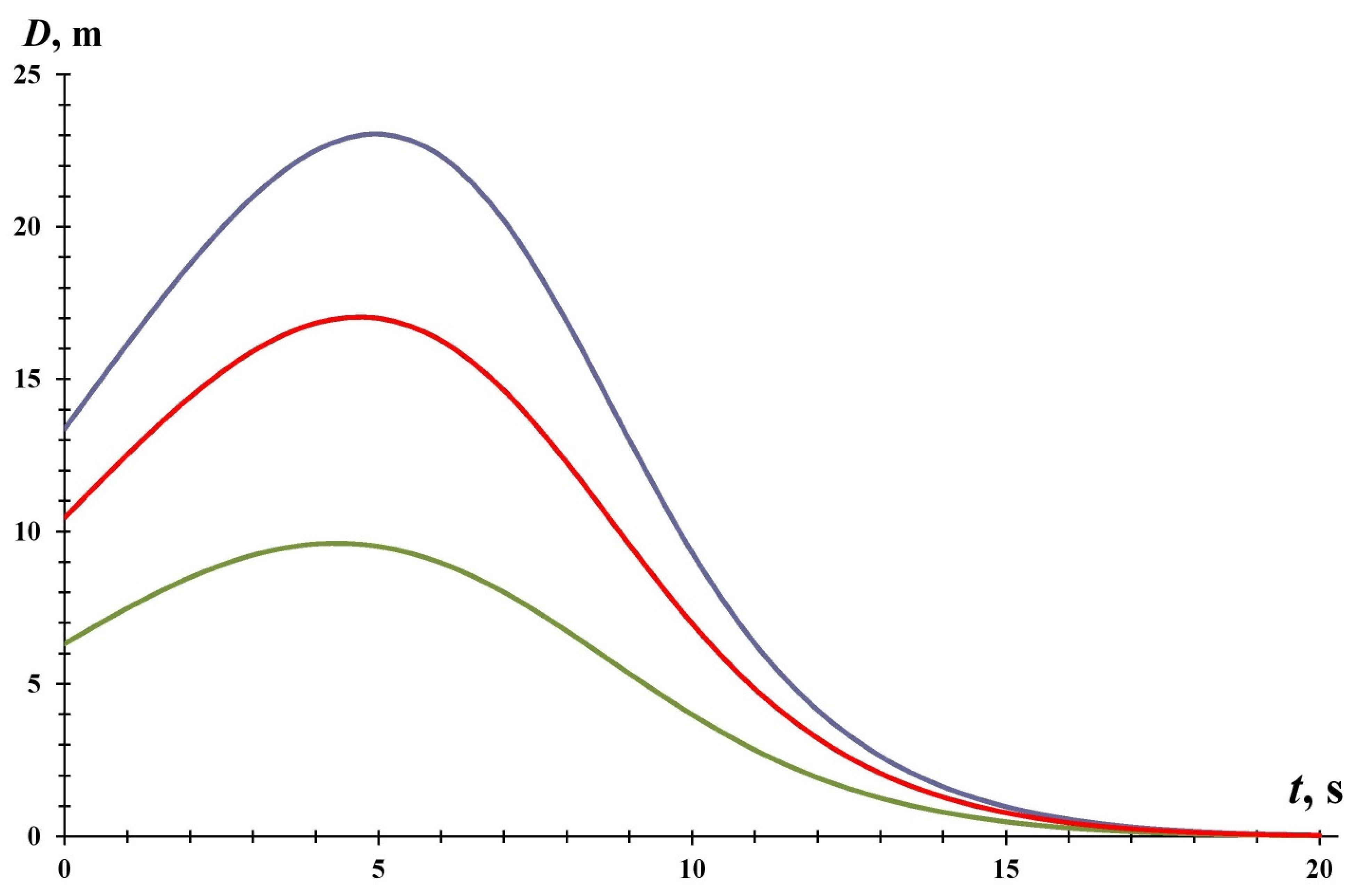
• A nonlinear problem with friction on the bottom has been solved. The resulting tsunami wave has an unusual dipole shape with two poles. A positive rise is adjacent to a negative decrease, with both poles moving together at the same velocity.

References

1. Arsen’yev, S.A.; Eppelbaum, L.V. Nonlinear model of coastal flooding by a highly turbulent tsunami. J. Nonlinear Math. Phys. 2021, 28, 436–451. [Google Scholar] [CrossRef]
2. Pelinovsky, E.N. Hydrodynamics of Tsunami Waves; Institute of Applied Physics of the Russia Academy of Science: Nizhny Novgorod, Russia, 1996. (In Russian) [Google Scholar]
3. Wendt, J.; Oglesby, D.D.; Geist, E.L. Tsunamis and splay fault dynamics. Geophys. Res. Lett. 2009, 36, L15303. [Google Scholar] [CrossRef]
4. Levin, B.W.; Nosov, M.A. Physics of Tsunami; Springer: Cham, Switzerland, 2016. [Google Scholar]
5. Rabinovich, A.B. Twenty-seven years of progress in the science of meteorological tsunamis following the 1992 Daytona Beach event. Pure Appl. Geophys. 2020, 177, 1193–1230. [Google Scholar] [CrossRef]
6. Arsen’yev, S.A.; Rykunov, L.N.; Shelkovnikov, N.K. Nonlinear interactions of tsunami and tides in an ocean. Dokl. Russ. Acad. Sci. 1993, 331, 732–734. [Google Scholar]
7. Turcotte, D.L. Fractals and Chaos in Geology and Geophysics; Cambridge University Press: Cambridge, UK, 1992. [Google Scholar]
8. Sadovsky, M.A. Some Selected Works. In Geophysics and Physics of Explosion; Nauka: Moscow, Russia, 1999. (In Russian) [Google Scholar]
9. Kardashov, V.R.; Eppelbaum, L.V.; Vasilyev, O.V. The role of nonlinear source terms in geophysics. Geophys. Res. Lett. 2000, 27, 2069–2072. [Google Scholar] [CrossRef] [Green Version]
10. Eppelbaum, L.V.; Kardashov, V.R. Analysis of strongly nonlinear processes in geophysics. In Proceedings of the Chapman Conference on Exploration Geodynamics, Dunsborough, Australia, 19–24 August 2001; pp. 43–44. [Google Scholar]
11. Keilis-Borok, V.; Ismail-Zadeh, A.; Kossobokov, V.; Shebalin, P. Non-linear dynamics of the lithosphere and intermediate-term earthquake prediction. Tectonophysics 2001, 338, 247–260. [Google Scholar] [CrossRef]
12. Morra, G.; Yuen, D.A. Role of Korteweg stresses in geodynamics. Geophys. Res. Lett. 2008, 35, L07304. [Google Scholar] [CrossRef]
13. Schmedes, J.; Archuleta, R.J.; Lavallèe, D. Correlation of earthquake source parameters inferred from dynamic rupture simulations. J. Geophys. Res. 2010, 115, B03304. [Google Scholar] [CrossRef] [Green Version]
14. Kakinuma, T. A Numerical Study on Distant Tsunami Propagation Considering the Strong Nonlinearity and Strong Dispersion of Waves, or the Plate Elasticity and Mantle Fluidity of Earth. Fluids 2022, 7, 150. [Google Scholar] [CrossRef]
15. Shuleikin, V.V. Physics of the Sea; Nauka: Moscow, Russia, 1968. (In Russian) [Google Scholar]
16. Sretensky, L.N. Theory of Wave Motions of Fluids; Nauka: Moscow, Russia, 1977. (In Russian) [Google Scholar]
17. Ablowitz, M.J.; Segur, H. Solitons and Inverse Spectral Transform; SIAM: Philadelphia, PA, USA, 1980. [Google Scholar]
18. Dodd, R.K.; Eilbeck, J.C.; Gibbon, J.D.; Morris, H.C. Solitons and Nonlinear Wave Equations; Academic Press: Cambridge, NY, USA, 1988. [Google Scholar]
19. Arsen’yev, S.A.; Seleverstov, S.V.; Shelkovnikov, N.K. Giant solitary waves in the ocean and their modeling. Mosc. Univ. Phys. Bull. 1997, 38, 57–59. [Google Scholar]
20. Ren, Z.; Liu, H.; Jimenez, C.; Wang, Y. Tsunami resonance and standing waves in the South China Sea. Ocean Eng. 2022, 262, 112323. [Google Scholar] [CrossRef]
21. Gao, J.; Ma, X.; Chen, H.; Zang, J.; Dong, G. On hydrodynamic characteristics of transient harbor resonance excited by double solitary waves. Ocean Eng. 2021, 219, 108345. [Google Scholar] [CrossRef]
22. Gao, J.; Ji, C.; Gaidai, O.; Liu, Y.; Ma, X. Numerical investigation of transient harbor oscillations induced by N-waves. Coast. Eng. 2017, 125, 119–131. [Google Scholar] [CrossRef]
23. Gao, J.; Ma, X.; Dong, G.; Zang, J.; Zhou, X.; Zhou, L. Topographic influences on transient harbor oscillations excited by N-waves. Ocean Eng. 2019, 192, 106548. [Google Scholar] [CrossRef]
24. Arsen’yev, S.A. On the theory of long waves on water. Dokl. Russ. Acad. Sci. 1994, 334, 635–638. [Google Scholar]
25. Geyer, A. Solitary traveling water waves of moderate amplitude. J. Nonlinear Math. Phys. 2012, 19 (Suppl. S1), 104–115. [Google Scholar] [CrossRef] [Green Version]
26. Rajan, G.K.; Bayram, S.; Henderson, D.M. Periodic envelopes of waves over non-uniform depth. Phys. Fluids 2016, 28, 042106. [Google Scholar] [CrossRef]
27. Benilov, E.S.; Flanagan, J.D.; Howlin, C.P. Evolution of packets of surface gravity waves over smooth topography. J. Fluid Mech. 2005, 533, 171–181. [Google Scholar] [CrossRef] [Green Version]
28. Grimshaw, R.H.J.; Annenkov, S.Y. Water wave packets over variable depth. Stud. Appl. Math. 2011, 126, 409–427. [Google Scholar] [CrossRef]
29. Fedorov, A.V.; Melville, W.K. Nonlinear gravity–capillary waves with forcing and dissipation. J. Fluid Mech. 1998, 354, 1–42. [Google Scholar] [CrossRef] [Green Version]
30. Arsen’yev, S.A.; Babkin, V.A.; Yu, G.A.; Nikolaevskiy, V.N. Theory of Mesoscale Turbulence. Eddies of the Atmosphere and the Ocean; Regular and Chaotic Dynamics, Institute of Computer Sciences: Moscow, Russia; Izhevsk, Russia, 2010. (In Russian) [Google Scholar]
31. Labzovskii, N.A. Non-Periodic Sea Level Fluctuations; Gidrometeoizdat: Saint Petersburg, Russia, 1971. (In Russian) [Google Scholar]
32. Arsen’yev, S.A. On the nonlinear equations of long sea waves. Water Resour. 1991, 1, 29–35. (In Russian) [Google Scholar]
33. Arsen’yev, S.A.; Shelkovnikov, N.K. Storm Surges as Dissipative Solitons. Mosc. Univ. Phys. Bull. 2013, 68, 483–489. [Google Scholar] [CrossRef]
34. Dwight, H.B. Tables of Integrals and Other Mathematical Data; Lan: Saint Petersburg, Russia, 2009. [Google Scholar]
35. Landau, L.D.; Lifshits, E.M. Fluid Mechanics; Pergamon Press: Oxford, UK; New York, NY, USA; Tokyo, Japan, 1987. [Google Scholar]
36. Whitham, F.R.S. Linear and Nonlinear Waves; John Wiley & Sons: New York, NY, USA; London, UK; Sydney, Australia, 1999. [Google Scholar]
37. Lighthill, J. Waves in Fluids; Cambridge University Press: London, UK; New York, NY, USA; Melbourne, Australia, 1978. [Google Scholar]
38. Johnson, R.S. Shallow Water Waves on a Viscous Fluid—The Undular Bore. Phys. Fluids 1972, 15, 1693–1699. [Google Scholar] [CrossRef]
39. El, G.A.; Grimshaw, R.H.J.; Smyth, N.F. Unsteady undular bores in fully non-linear shallow–water theory. Phys. Fluids 2006, 18, 027104. [Google Scholar] [CrossRef] [Green Version]
40. Vinogradova, M.B.; Rudenko, O.B.; Suhorukov, A.P. Theory of Waves; Nauka: Moscow, Russia, 1990. (In Russian) [Google Scholar]
41. Gurbatov, S.N.; Rudenko, O.V.; Saichev, A.I. Waves and Structures in Nonlinear Media without Dispersion. Applications to Nonlinear Acoustics; Fizmatlit: Moscow, Russia, 2008. (In Russian) [Google Scholar]
42. Tikhonov, N.; Samarsky, A.A. Equations of Mathematical Physics; Moscow University Press: Moscow, Russia, 1999. [Google Scholar]
43. Arsen’yev, S.A. On the laws of resistance for purely drift and gradient flows. In Comprehensive Studies of the Northern Caspian; Institute of Water Problems, Academy of Sciences of the USSR: Moscow, Russia; Nauka: Moscow, Russia, 1988. (In Russian) [Google Scholar]
44. Kolmogorov, A.N. Equations of turbulent motion of an incompressible fluid. Izv. USSR Acad. Sci. Phys. Ser. 1942, 6, 299–303. (In Russian) [Google Scholar]
Figure 1. Simplified scheme: horizontal coordinate axes and symbols (modified after [1]).
Applsci 13 08112 g001
Figure 2. Schematic vertical section of the water flow over the bottom relief (modified after [1]).
Applsci 13 08112 g002
Figure 3. Calculations of a switching wave (kink) arriving at a given shelf point x = 100 m. The curves correspond to different values of the turbulent viscosity coefficient AL. The blue curve is calculated at AL = 10 m2/s, the red curve is calculated at AL = 100 m2/s, and the green curve is calculated at AL = 1000 m2/s.
Applsci 13 08112 g003
Figure 4. The forms of arriving tsunami waves are calculated by Equations (25)–(29) for various values of the parameter p determined by the initial conditions. Green curve, p = 0.8; blue curve, p = 0.6; and red curve, p = 0.4.
Applsci 13 08112 g004
Figure 5. Dissipative tsunami solitons are calculated by Equation (31) for various values of the constant A. Dark blue curve at A = 3, red curve at A = 4, and green curve at A = 7. The ratio between the dimensional coordinates in Figure 5 and nondimensional variables in Equation (31) are the following: Z = ς/ς*, D = −ς, α = −τ, τ = (TX), T = ωt, X = kx = ωx/c0, and λ = FL/2, FL = ωAL/c02.
Applsci 13 08112 g005
Figure 6. Dipole tsunami waves calculated by Equation (37) with initial amplitude ζ0 = 1 m. Wave behavior is shown at the following distances from the shelf edge: x = 100 m (blue curve) and x = 500 m (red curve).
Applsci 13 08112 g006
Disclaimer/Publisher’s Note: The statements, opinions and data contained in all publications are solely those of the individual author(s) and contributor(s) and not of MDPI and/or the editor(s). MDPI and/or the editor(s) disclaim responsibility for any injury to people or property resulting from any ideas, methods, instructions or products referred to in the content.