
Safety Assessment and Uncertainty Quantification of Electromagnetic Radiation from Mobile Phones to the Human Head

Abstract
1. Introduction
2. Parameter Uncertainty Quantification Method
2.1. gPC Method
2.2. Random Response Surface Method
- a.
- Construction of the generalized chaotic polynomial expansion model
- b.
- Estimation of the coefficient of interest
2.3. Global Sensitivity Analysis
3. Electromagnetic Simulation Model and Electromagnetic Radiation Scenarios
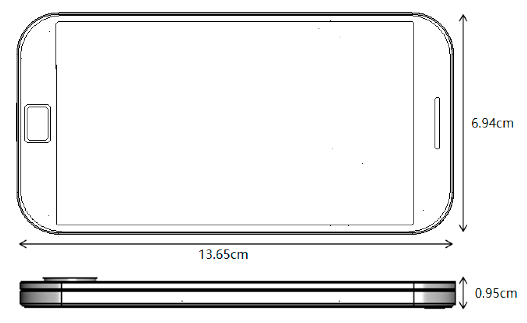
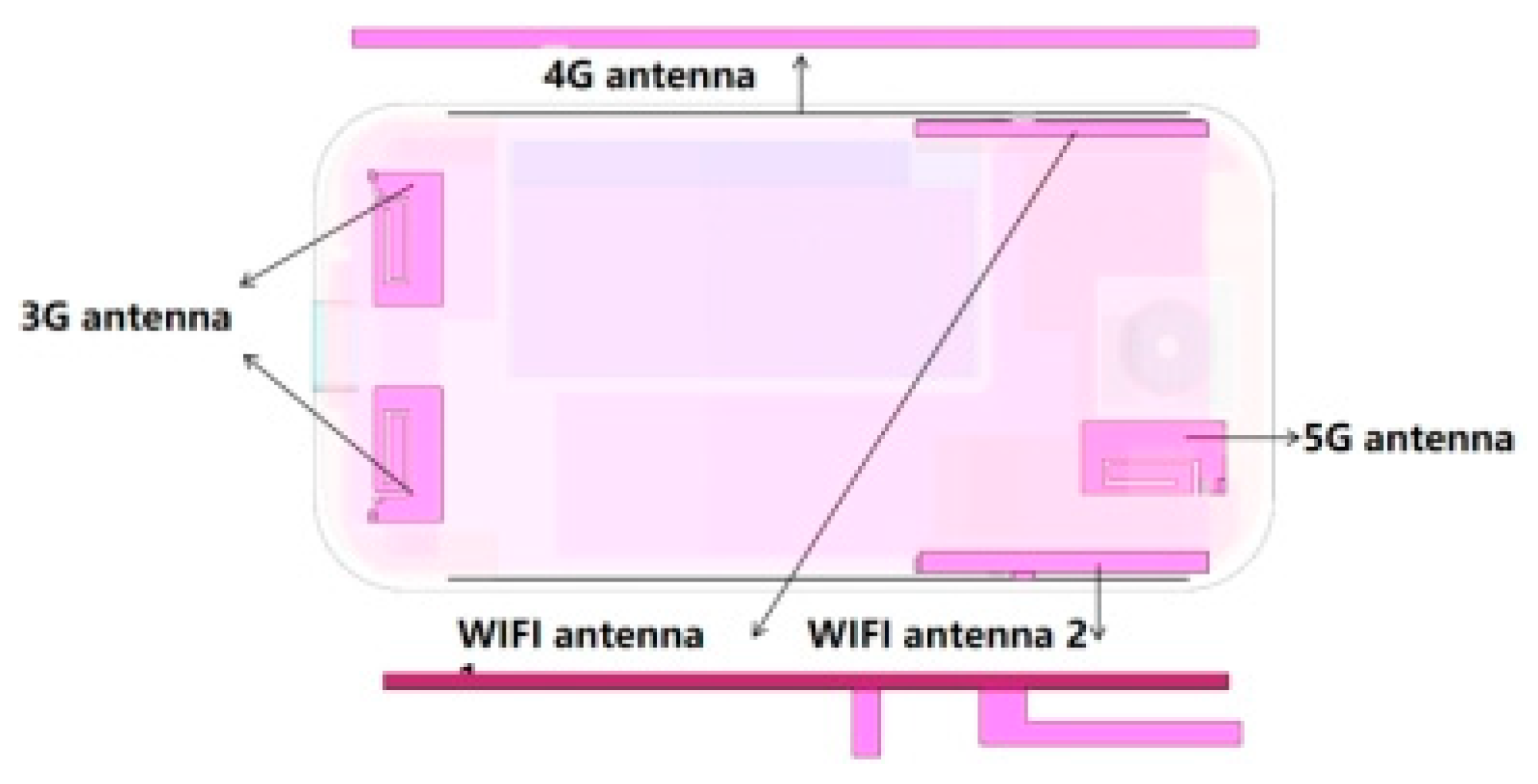
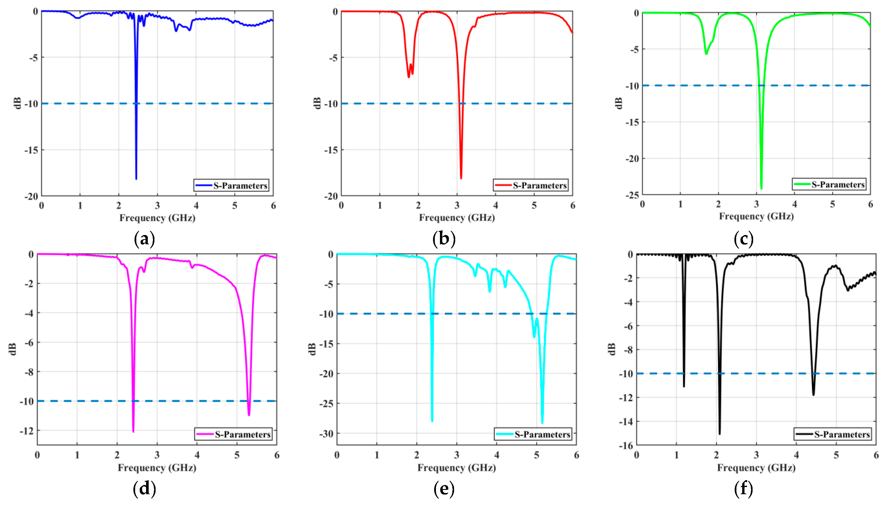
3.1. Mobile Phone Electromagnetic Simulation Model
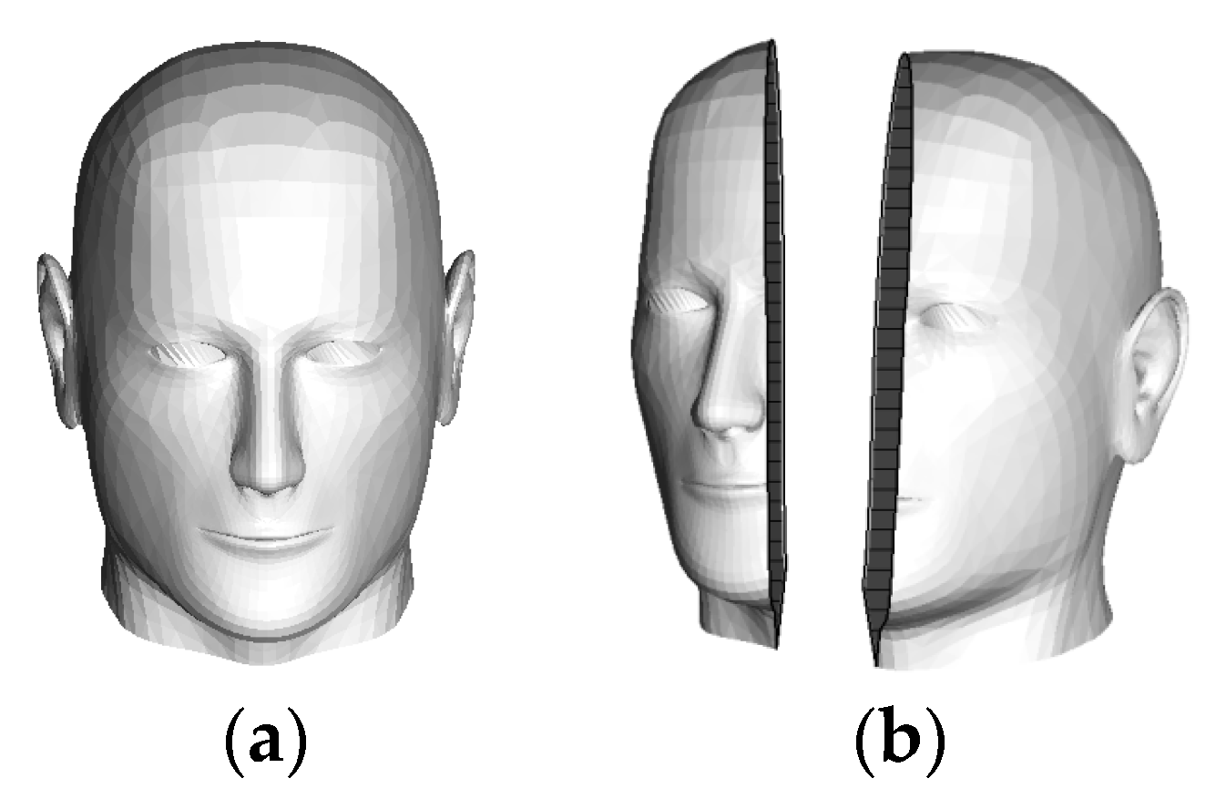
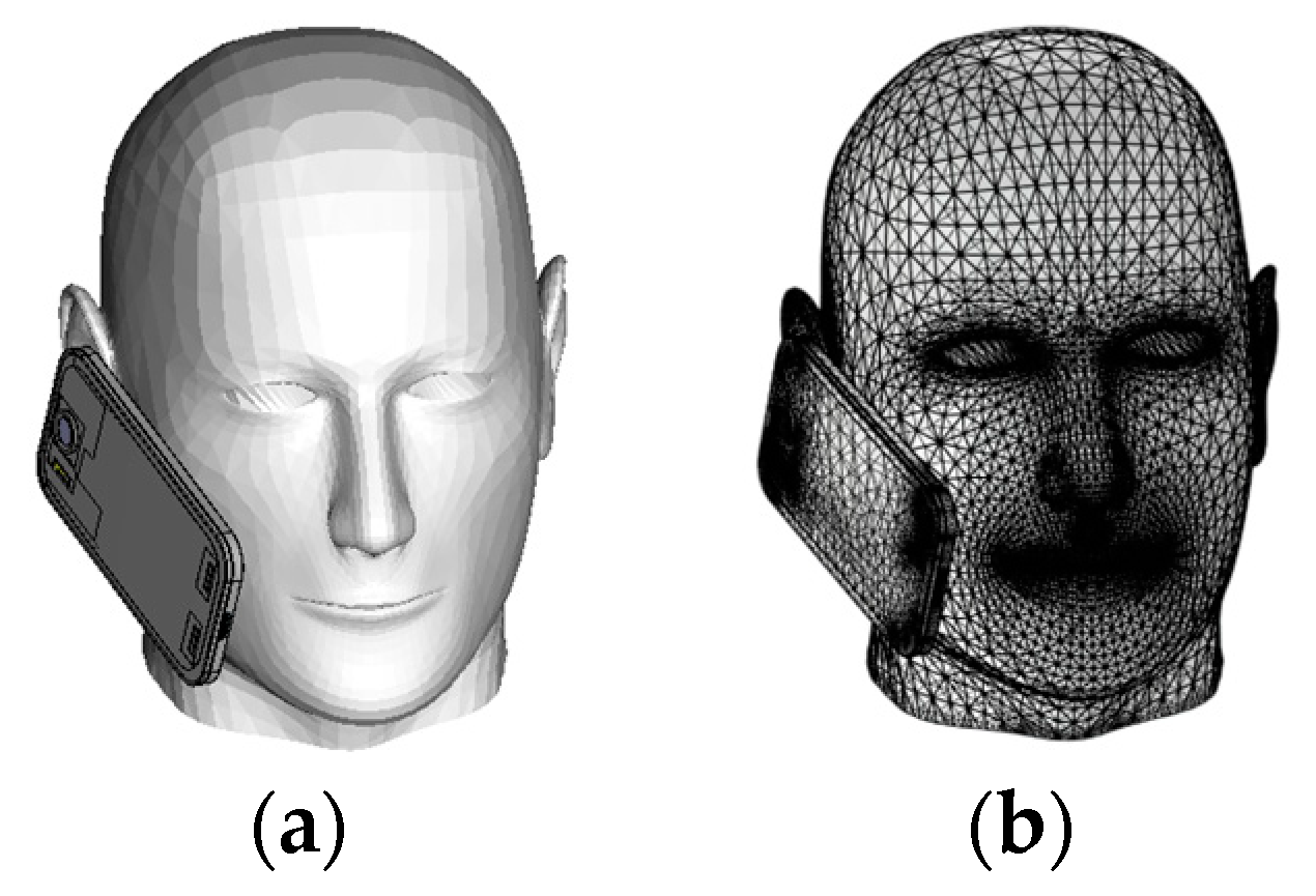
3.2. Electromagnetic Simulation Model of the Human Head
3.3. Electromagnetic Radiation Scenarios
4. Electromagnetic Exposure Safety Assessment and Uncertainty Quantification
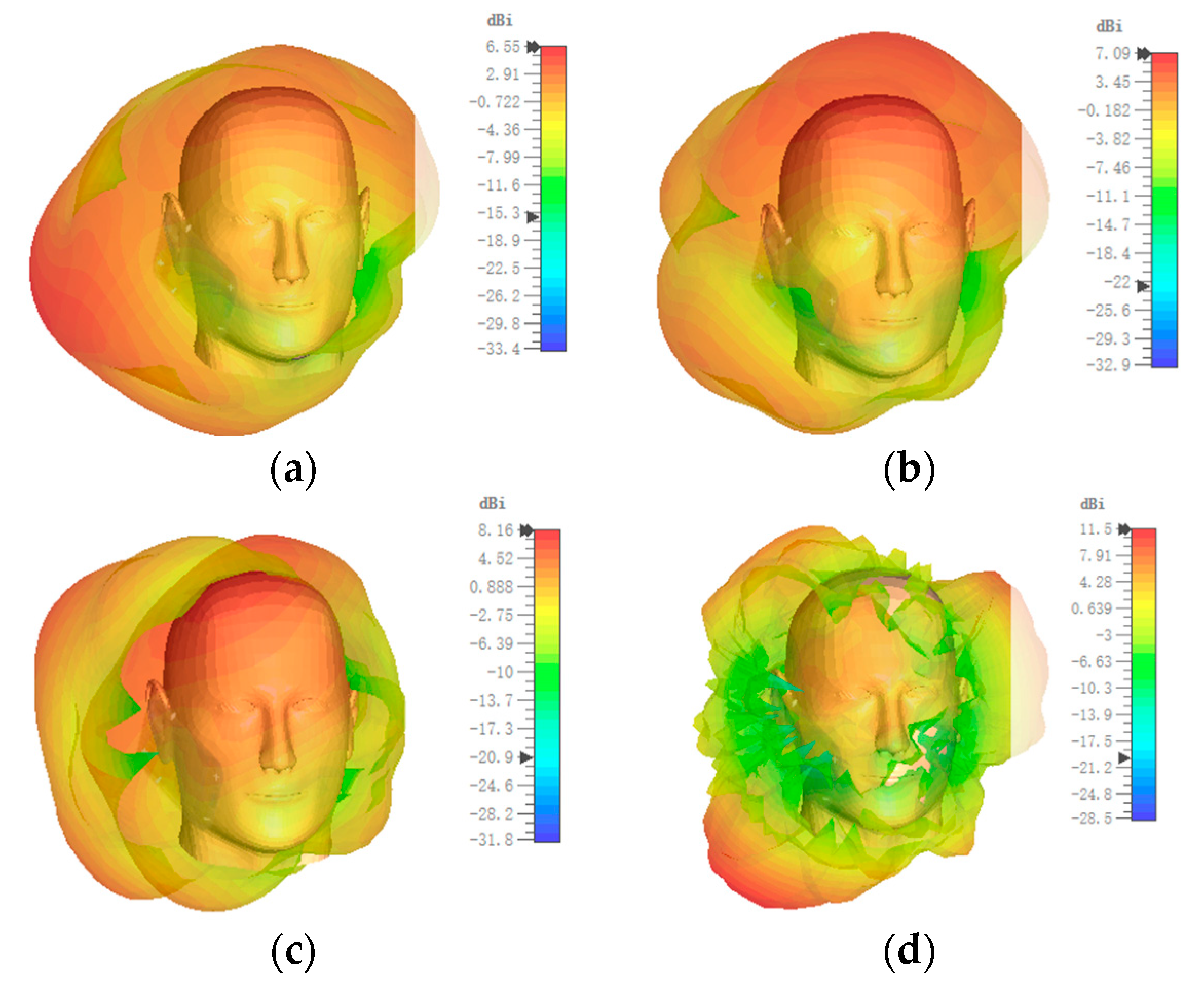
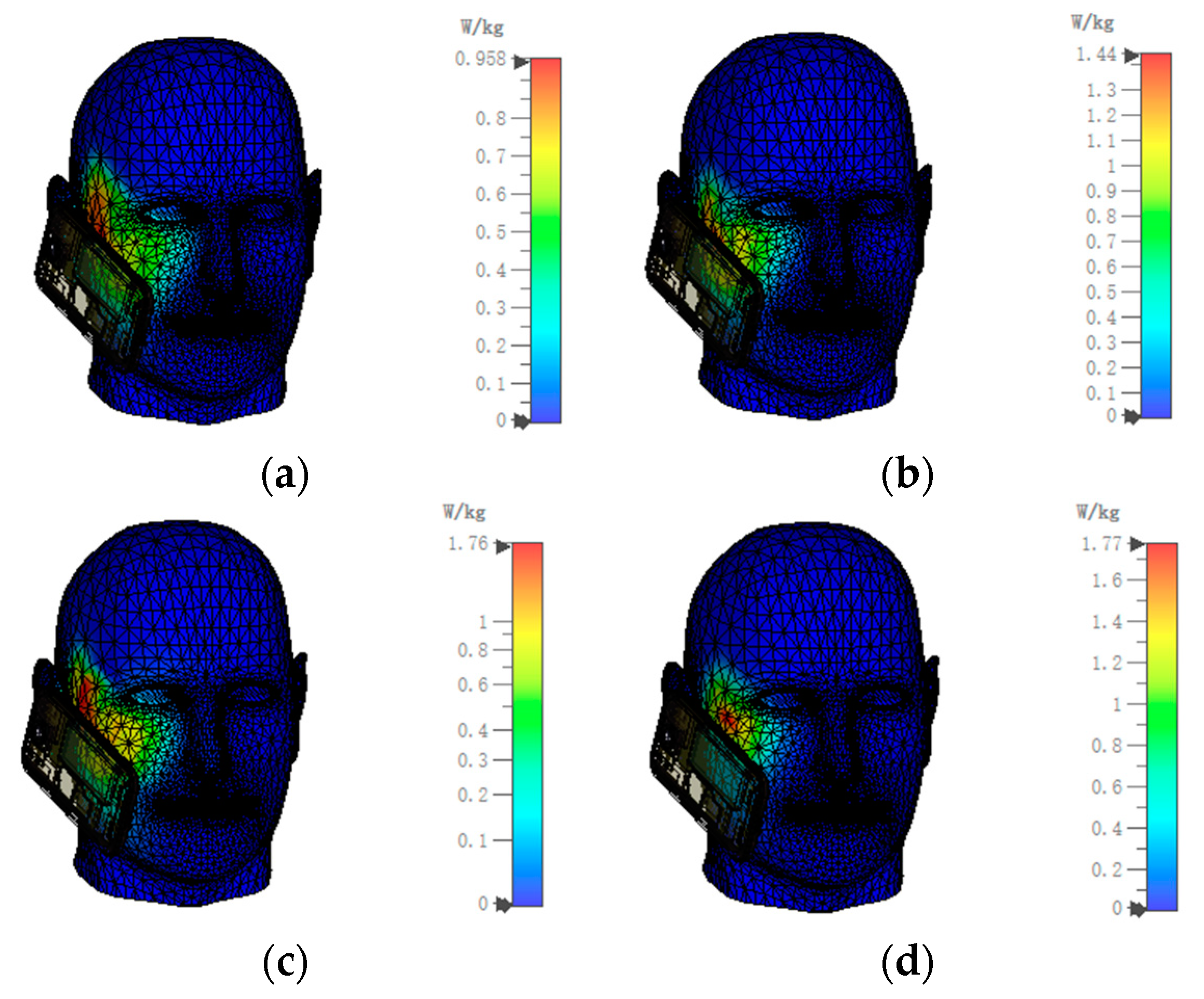
4.1. Safety Assessment
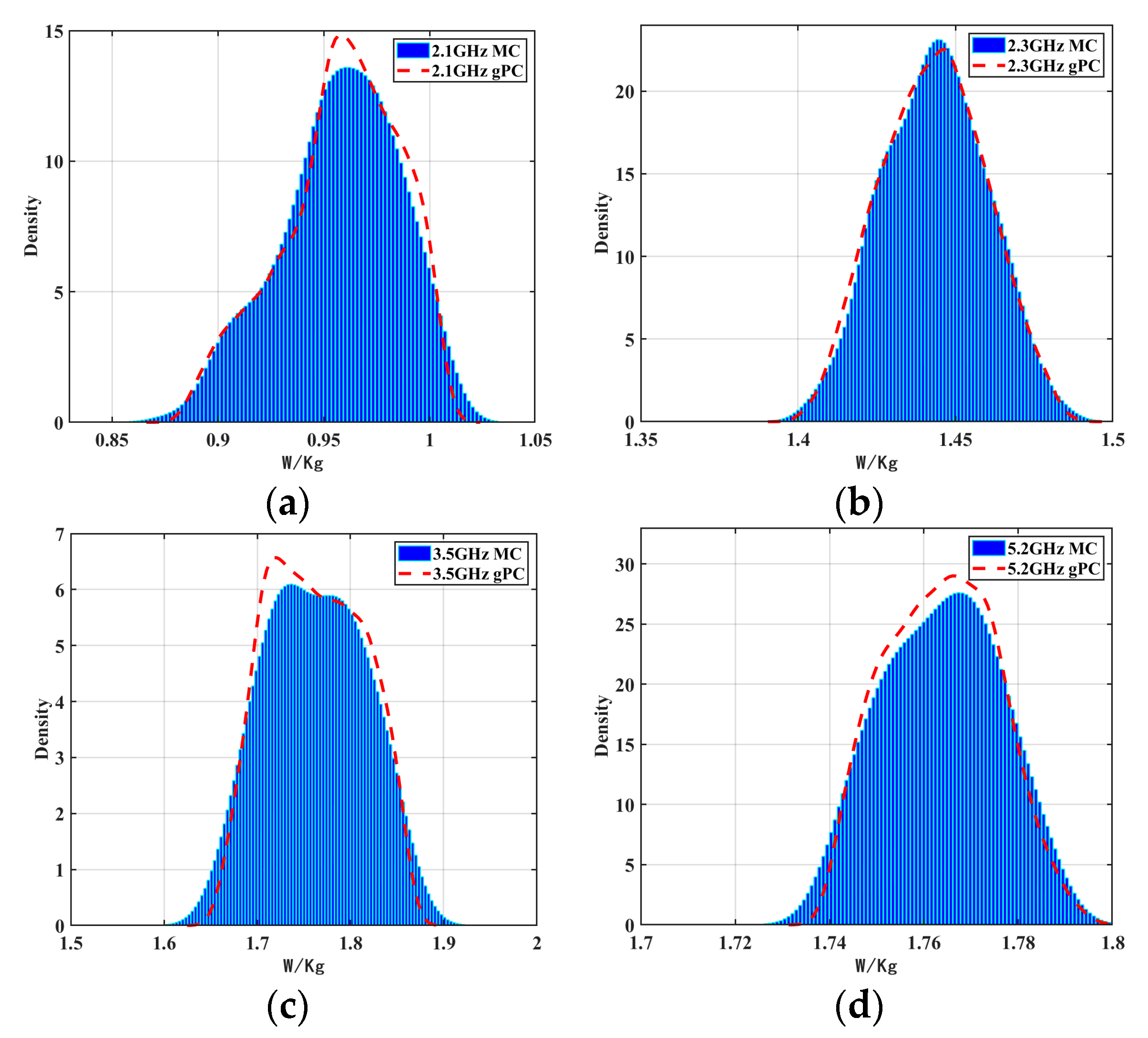
4.2. Uncertainty Quantification
5. Conclusions
Author Contributions
Funding
Institutional Review Board Statement
Informed Consent Statement
Data Availability Statement
Acknowledgments
Conflicts of Interest
References
- van Rongen, E.; Croft, R.; Juutilainen, J.; Lagroye, I.; Miyakoshi, J.; Saunders, R.; de Seze, R.; Tenforde, T.; Verschaeve, L.; Veyret, B.; et al. Effects of radiofrequency electromagnetic fields on the human nervous system. J. Toxicol. Environ. Health Part B 2009, 12, 572–597. [Google Scholar] [CrossRef] [PubMed]
- Kesari, K.K.; Siddiqui, M.; Meena, R.; Verma, H.N.; Kumar, S. Cell phone radiation exposure on brain and associated biological systems. Indian J. Exp. Biol. 2013, 51, 187–200. [Google Scholar] [PubMed]
- Mumtaz, S.; Rana, J.N.; Choi, E.H.; Han, I. Microwave Radiation and the Brain: Mechanisms, Current Status, and Future Prospects. Int. J. Mol. Sci. 2022, 23, 9288. [Google Scholar] [CrossRef] [PubMed]
- Gartshore, A.; Kidd, M.; Joshi, L.T. Applications of Microwave Energy in Medicine. Biosensors 2021, 11, 96. [Google Scholar] [CrossRef]
- IEEE Standard 1528-2013; IEEE Recommended Practice for Determining the Peak Spatial-Average Specific Absorption Rate (SAR) in the Human Head from Wireless Communications Devices: Measurement Techniques. IEEE: Piscataway, NY, USA, 2013.
- International Commission on Non-Ionizing Radiation Protection. Guidelines for limiting exposure to time-varying electric, magnetic and electromagnetic fields (up to 300 GHz). Health Phys. 1998, 75, 494–522. [Google Scholar]
- Zhou, W.; Lu, M. Safety evaluation of radio frequency electromagnetic exposure from wireless communication system of subway. J. Radiat. Res. Radiat. Process. 2018, 36, 040401. [Google Scholar]
- IS/IEC 62209-1; Human Exposure to Radio Frequency Fields from Hand-Held and Body-Mounted Wireless Communication Devices—Human Models, Instrumentation, and Procedures—Part 1: Procedure to Determine the Specific Absorption Rate (SAR) for Hand-Held Devices Used in Close Proximity to the Ear (Frequency Range of 300 MHz to 3 GHz). IEC: Geneva, Switzerland, 2005.
- Singh, M. Biological heat and mass transport mechanisms behind nanoparticles migration revealed under microCT image guidance. Int. J. Therm. Sci. 2023, 184, 107996. [Google Scholar] [CrossRef]
- Singh, M.; Ma, R.; Zhu, L. Quantitative evaluation of effects of coupled temperature elevation, thermal damage, and enlarged porosity on nanoparticle migration in tumors during magnetic nanoparticle hyperthermia. Int. Commun. Heat Mass Transf. 2021, 126, 105393. [Google Scholar] [CrossRef]
- Cheng, X.; Monebhurrun, V. Application of different methods to quantify uncertainty in specific absorption rate calculation using a CAD-based mobile phone model. IEEE Trans. Electromagn. Compat. 2016, 59, 14–23. [Google Scholar] [CrossRef]
- Xiu, D. The wiener-asky polynomial chaos for stochastic differential equations. SIAM J. Sci. Comput. 2005, 27, 1118–1139. [Google Scholar] [CrossRef]
- Xiu, D.; Karniadakis, G.E. Modeling uncertainty in flow simulations via generalized polynomial chaos. J. Comput. Phys. 2003, 187, 137–167. [Google Scholar] [CrossRef]
- Rubinstein, R.Y.; Kroese, D.P. (Eds.) Simulation and Monte Carlo Method; Front Matter; John Wiley & Sons: Hoboken, NJ, USA, 2008. [Google Scholar]
- Blatman, R.; Sudret, B. Adaptive sparse polynomial chaos expansion based on least angle regression. J. Comput. Phys. 2011, 230, 2345–2367. [Google Scholar] [CrossRef]
- Marelli, S.; Sudret, B. An active-learning algorithm that combines sparse polynomial chaos expansions and bootstrap for structural reliability analysis. Struct. Saf. 2018, 75, 67–74. [Google Scholar] [CrossRef]
- Kersaudy, P.; Sudret, B.; Varsier, N.; Picon, O.; Wiart, J. A new surrogate modeling technique combining Kriging and polynomial chaos expansions—Application to uncertainty analysis in computational dosimetry. J. Comput. Phys. 2015, 286, 103–117. [Google Scholar] [CrossRef]
- Jakeman, J.D.; Eldred, M.S.; Sargsyan, K. Enhancing l(1)-minimization estimates of polynomial chaos expansions using basis selection. J. Comput. Phys. 2015, 289, 18–34. [Google Scholar] [CrossRef]
- Homma, T.; Saltelli, A. Importance measures in global sensitivity analysis of nonlinear models. Reliab. Eng. Syst. Saf. 1996, 52, 1–17. [Google Scholar] [CrossRef]
- Isukapalli, S.S. Uncertainty Analysis of Transport-Transformation Models. Ph.D. Thesis, The State University of New Jersey, New Brunswick, NJ, USA, 1999. [Google Scholar]
- IEEE P62704-3; Determining the Peak Spatial-Average Specific Absorption Rate (SAR) in the Human Body from Wireless Communications Devices, 30 MHz–6 GHz. Part 3: Specific Requirements for Using the Finite-Difference Time-Domain (FDTD) Method for SAR Calculations of Mobile Phones. IEEE: Piscataway, NY, USA, 2020.
- Monebhurrun, V.; Wong, M.F.; Wiart, J. Numerical and experimental investigations of a commercial mobile handset for SAR calculations. In Proceedings of the 2nd International Conference on Bioinformatics and Biomedical Engineering, Shanghai, China, 16–18 May 2008; pp. 784–787. [Google Scholar]
- CST Studio Suite. Electromagnetic Field Simulation Software. Available online: https://www.3ds.com/products-services/simulia/products/cst-studio-suite (accessed on 14 May 2021).
- IEC/IEEE 62704-1; IEC/IEEE International Standard—Determining the Peak Spatial-Average Specific Absorption Rate (SAR) in the Human Body from Wireless Communications Devices, 30 MHz to 6 GHz—Part 1: General Requirements for Using the Finite-Difference Time-Domain (FDTD) Method for SAR Calculations. IEEE: Piscataway, NY, USA, 2017; pp. 1–86.
- Gabriel, C. Compilation of the Dielectric Properties of Body Tissues at RF and Microwave Frequencies; Report AL/OE-TR-1996-0037; Armstrong Laboratory (AFMC), Radiofrequency Radiation Division, Brooks AFB: San Antonio, TX, USA, 1996. [Google Scholar]
- Gabriel, C.; Gabriel, S.; Corthout, E. The dielectric properties of biological tissues: I. Literature survey. Phys. Med. Biol. 1996, 41, 2231–2249. [Google Scholar] [CrossRef] [PubMed]
- Gabriel, S.; Lau, R.W.; Gabriel, C. The dielectric properties of biological tissues: II. Measurements in the frequency range 10 Hz to 20 GHz. Phys. Med. Biol. 1996, 41, 2251–2269. [Google Scholar] [CrossRef]
- Gabriel, S.; Lau, R.W.; Gabriel, C. The dielectric properties of biological tissues: III. Parametric models for the frequency spectrum of tissues. Phys. Med. Biol. 1996, 41, 2271–2293. [Google Scholar] [CrossRef]
- Duck, F.A. Physical Properties of Tissue—A Comprehensive Reference Book; Academic Press Ltd.: Cambridge, MA, USA, 1990. [Google Scholar]
- Singh, M.; Gu, Q.; Ma, R.; Zhu, L. Heating Protocol Design Affected by Nanoparticle Redistribution and Thermal Damage Model in Magnetic Nanoparticle Hyperthermia for Cancer Treatment. J. Heat Transf. 2020, 142, 072501. [Google Scholar] [CrossRef]
- Stein, M. Large Sample Properties of Simulations Using Latin Hypercube Sampling. Technometrics 1987, 29, 143–151. [Google Scholar] [CrossRef]


| Distribution Pattern | Orthogonal Polynomial Basis | Weight Function | Variable Range | |
|---|---|---|---|---|
| normal | Hermite | |||
| uniform | 1/2 | Legendre | 1 | |
| exponential | Legendre | |||
| γ | generalized Legendre |
| Component | Relative Permittivity | Conductivity |
|---|---|---|
| antenna | 1.00 | PEC |
| battery | 1.00 | PEC |
| battery jar | 5.00 | PEC |
| display screen | 4.80 | 0.01 |
| PCB | 1.00 | PEC |
| phone receiver | 1.00 | PEC |
| loudspeaker | 1.00 | PEC |
| speaker connector | 1.00 | PEC |
| inner shell | 2.30 | PEC |
| shell | 2.20 | PEC |
| camera | 1.90 | PEC |
| casing pipe | 3.00 | 0.01 |
| vibrator | 1.00 | PEC |
| Dielectric Constant | Distribution Pattern | Distribution Interval |
|---|---|---|
| camera | uniform | [1.8,2.0] |
| battery jar | uniform | [4.8,5.2] |
| inner shell | normal | [2.3,0.52] |
| shell | uniform | [2.0,2.4] |
| Frequency | Output Mean | Standard Deviation | ||
|---|---|---|---|---|
| MC | gPC | MC | gPC | |
| 2.1 GHz | 0.9576 | 0.9580 | 0.0274 | 0.0277 |
| 2.3 GHz | 1.4436 | 1.4431 | 0.0159 | 0.0165 |
| 3.5 GHz | 1.7621 | 1.7622 | 0.0511 | 0.0501 |
| 5.2 GHz | 1.7737 | 1.7731 | 0.0119 | 0.0117 |
| Frequency | 2.1 GHz | 2.3 GHz | 3.5 GHz | 5.2 GHz |
|---|---|---|---|---|
| mean | 0.9580 | 1.4431 | 1.7622 | 1.7731 |
| STD | 0.0277 | 0.0165 | 0.0501 | 0.0117 |
| minimum | 0.8804 | 1.3993 | 1.6557 | 1.7380 |
| maximum | 1.0098 | 1.4885 | 1.8662 | 1.8078 |
| lower 90% | 0.9051 | 1.4159 | 1.6846 | 1.7548 |
| upper 90% | 0.9985 | 1.4706 | 1.8443 | 1.7928 |
| lower 95% | 0.8978 | 1.4122 | 1.6756 | 1.7529 |
| upper 95% | 1.0019 | 1.4749 | 1.8513 | 1.7962 |
| lower 99% | 0.8885 | 1.4056 | 1.6633 | 1.7502 |
| upper 99% | 1.0062 | 1.4807 | 1.8607 | 1.8016 |
| Computational Method | Computation Time |
|---|---|
| gPC | 35 min 20 s |
| MC | 16 h 36 min |
Disclaimer/Publisher’s Note: The statements, opinions and data contained in all publications are solely those of the individual author(s) and contributor(s) and not of MDPI and/or the editor(s). MDPI and/or the editor(s) disclaim responsibility for any injury to people or property resulting from any ideas, methods, instructions or products referred to in the content. |
© 2023 by the authors. Licensee MDPI, Basel, Switzerland. This article is an open access article distributed under the terms and conditions of the Creative Commons Attribution (CC BY) license (https://creativecommons.org/licenses/by/4.0/).
Share and Cite
Yi, M.; Wu, B.; Zhao, Y.; Su, T.; Chi, Y. Safety Assessment and Uncertainty Quantification of Electromagnetic Radiation from Mobile Phones to the Human Head. Appl. Sci. 2023, 13, 8107. https://doi.org/10.3390/app13148107
Yi M, Wu B, Zhao Y, Su T, Chi Y. Safety Assessment and Uncertainty Quantification of Electromagnetic Radiation from Mobile Phones to the Human Head. Applied Sciences. 2023; 13(14):8107. https://doi.org/10.3390/app13148107
Chicago/Turabian StyleYi, Miao, Boqi Wu, Yang Zhao, Tianbo Su, and Yaodan Chi. 2023. "Safety Assessment and Uncertainty Quantification of Electromagnetic Radiation from Mobile Phones to the Human Head" Applied Sciences 13, no. 14: 8107. https://doi.org/10.3390/app13148107
APA StyleYi, M., Wu, B., Zhao, Y., Su, T., & Chi, Y. (2023). Safety Assessment and Uncertainty Quantification of Electromagnetic Radiation from Mobile Phones to the Human Head. Applied Sciences, 13(14), 8107. https://doi.org/10.3390/app13148107