Solution for the Mathematical Modeling and Future Prediction of the COVID-19 Pandemic Dynamics

Abstract

The COVID-19 infectious disease spread in the world represents, by far, one of the most significant moments in humankind’s recent history, affecting daily activities for a long period of time. The data available now allow important modelling developments for the simulation and prediction of the process of an infectious disease spread. The current work provides strong insight for estimation and prediction mathematical model development with emphasis on differentiation between three distinct methods, based on data gathering for Romanian territory. An essential aspect of the research is the quantification and filtering of the collected data. The current work identified five main categories considered as the model’s inputs: inside temperatures (°C), outside temperatures (°C), humidity (%), the number of tests and the quantified value of COVID-19 measures (%) and, as the model’s outputs: the number of new cases, the number of new deaths, the total number of cases or the total number of deaths. Three mathematical models were tested to find the optimal solution: transfer vector models using transfer functions as elements, autoregressive-exogenous (ARX) models, and autoregressive-moving-average (ARMAX) models. The optimal solution was selected by comparing the fit values obtained after the simulation of all proposed models. Moreover, the manuscript includes a study of the complexity of the proposed models. Based on the gathered information, the structure parameters of the proposed models are determined and the validity and the efficiency of the obtained models are proven through simulation.

1. Introduction

Very few phenomena throughout human history have shaped our societies and cultures the way outbreaks of infectious diseases have. Catastrophic pandemics have occurred at regular intervals throughout human history. The bubonic plague of the 14th century, within 50 years of its reign, reduced the global population from 450 million, possibly, to below 300 million, and may have claimed up to 60% of the lives in Europe at that time [1,2]. The Spanish flu pandemic (1918–1920) was the first true global pandemic that occurred in the setting of modern medicine, with specialities such as infectious diseases and epidemiology studying the nature of the illness and the course of the pandemic as it unfolded [3]. A fifth of the world’s population, at that time, was infected and 50 million people worldwide were killed. An unusual characteristic of this virus was the high death rate it caused among healthy adults from 15 to 34 years of age [4]. Severe Acute Respiratory Syndrome (SARS) was the first outbreak in the twenty-first century that managed to receive public attention. Caused by the SARS Coronavirus (SARS-CoV), the first cases originated in China and affected fewer than 10,000 individuals, but the severity of respiratory symptoms and mortality rate of about 10% caused a global public health concern. Due to the vigilance of public health systems worldwide, the outbreak was contained by mid-2003 [5]. The 2009 H1N1 influenza pandemic infected over 10% of the global population; it was perceived as highly threatening because it disproportionately affected healthy young adults, often quickly leading to severe respiratory failure [6].

COVID-19 is an infectious disease caused by the SARS-CoV-2 virus. In December 2019, the illness was first reported in Wuhan, the capital of China’s Hubei province. At the end of December 2019, a consistent number of patients were admitted to hospitals with an initial pneumonia diagnostic test showing an unknown etiology [7], soon confirmed as a previously unknown betacoronavirus, different from both MERS-CoV and SARS-CoV, and the seventh member of the family of coronaviruses that infect humans [8]. Since then, the disease caused by SARS-CoV-2, COVID-19, has spread around the globe. COVID-19 was declared a global pandemic on 11 March 2020 by the World Health Organization (WHO) [9].

Coronaviruses are among the main pathogens that predominantly affect the human respiratory system. SARS-CoV-2 is mainly spread via respiratory droplets, including aerosols, from a COVID-19-infected person who sneezes, coughs, speaks, sings, or breathes near other people. Exposure may occur via the inhalation of respiratory droplets or aerosol particles, deposition of respiratory droplets and particles on exposed mucous membranes (mouth, nose and eyes) and/or by touching mucous membranes after being contaminated by contact with surfaces with the infectious virus on them. The relative risk of environmental SARS-CoV-2 transmission from contaminated surfaces is considered low compared with direct contact, droplet transmission, or airborne transmission [10].

The WHO updated regularly guidance on critical preparedness, readiness and response for actions that are necessary (depending on the SARS-CoV-2 transmission scenario), such as contact tracing, laboratory testing, infection prevention and control, public health and social measures and health services [11,12]. Environmental factors, such as air pollution and chemical exposures, climate, and the built environment, were found to influence COVID-19 transmission and coronavirus disease 2019 (COVID-19) susceptibility and severity through four major interlinking mechanisms: increased risk of preexisting conditions associated with disease severity; immune system impairment; viral survival and transport; and behaviours that increase viral exposure [12]. Several studies have pointed to comorbidities as key factors in the prognosis of COVID-19 cases. Cancer, older age, cardiovascular diseases, and certain cardiovascular risk factors including hypertension, diabetes mellitus, renal disease, liver disease, cerebrovascular disease, obesity, smoking history and current smoking associated with a higher likelihood of severe COVID-19 and/or mortality with COVID-19 [13,14].

In the face of the current time-sensitive COVID-19 pandemic, the limited capacity of healthcare systems resulted in an emerging need for newer methods to control the pandemic spread to be developed. Artificial Intelligence (AI), and Machine Learning (ML) have a vast potential to exponentially optimize healthcare research. AI-based tools can be a game-changer for the diagnosis, treatment, and management of COVID-19 patients with the potential to reshape the future of healthcare [15,16].

The first case of COVID-19 was diagnosed in Romania on 26 February 2020 [17]. Due to the spread of COVID-19 in Italy, the government of Romania and the National Institute of Public Health decided at the beginning of March 2020 to have a two-week quarantine period and SARS-CoV-2 molecular testing for all individuals coming from the risk regions [18]. Other healthcare measures included designating five tertiary infectious diseases hospitals as facilities dedicated to COVID-19 treatments and assigning specific microbiology laboratories for molecular diagnostic testing. To reduce virus transmission, several other steps were taken by the government and the National Emergency Situations Committee, such as suspending school activities, restrictions for large mass gatherings and border closures.

The number of affected people reached the first hundred at the end of the second week of March 2020. Following an increase in new affirmed cases, on 24 March, the administration declared Military Ordinance, establishing a national lockdown. By 4 April 2020, there were 181 COVID-19 deaths reported [19].

As with many other processes in nature, from the growth of a bacterial colony to the spread of SARS-CoV-2, processes that vary in time, COVID-19 can be described with the help of mathematical functions (linear, nonlinear, exponential, parabolic, polynomial, logarithmic, etc.) some simpler, others complex [20]. The major challenge for any researcher is to identify which function captures most accurately the dynamics of the analyzed nature process (the evolution of the HIV epidemic in the 1980s was well captured by polynomial functions) [21].

Approximately two months after the first COVID-19 diagnosed case in Romania, the number of COVID-19 infected people announced by the authorities exceeded the level of 10,000 cases, while, by 2023, at the end of January, 3.32 million confirmed cases and 67,542 confirmed deaths were reported [22]. Probably, this number is lower than the real one based on the multitude of factors that influenced the pandemic spread and this possibility was considered in the design of our complex mathematical model.

Other prediction models regard the COVID-19 spread in four European countries (Spain, Germany, France and Italy). The forecasts of future COVID-19 daily cases in [23,24] have a prediction interval of 10 days. Both performed studies used the ARIMA model (autoregressive integrated moving average). Those studies show that ARIMA models are suitable for predicting the prevalence of COVID-19 in the future; the results are analyzed to understand the trends of the outbreak, in the given countries.

The model with the fewest parameters is most likely the susceptible-infected-removed (SIR) model, which is based on dividing the population into the following groups: susceptible (S) individuals are those who are not affected; infected and infectious individuals (I) with more or less visible symptoms; people who have been removed (R) from the infectious process, either because they have been cured or because they have died after being infected [25].

Another study uses the SIHM model, a model adding the feedback and memory into an SI (R) model, for describing the COVID-19 dynamics [26], considering values as susceptible individuals (S), the infectious (I), hospital admissions (H) and a memory (M) variable retaining the average number of admissions inside hospitals, for four countries in Europe (Germany, France, UK and Italy).

In recent studies, different data-driven models have been used to predict infections [27,28], using methods with different approaches including machine learning [29], search-interest-based models [30], neural networks and artificial intelligence. A neural network approach is considered one of the most efficient prediction models in building a medical classification [31]. Such a neural network was used to generate a classifier prediction model to foresee the status of recovered and death associated with COVID-19 patients [31].

Artificial intelligence (AI) was used in other types of applications for COVID-19 for looking ahead against the new diseases: monitoring the treatment, individuals contact tracing, projection of cases and mortality or drug research [32,33]. AI is a technology which can easily track the spread of this virus and can be useful in controlling this infection in real-time; with the help of real-time data analysis, AI can provide updated information also helping its prevention. 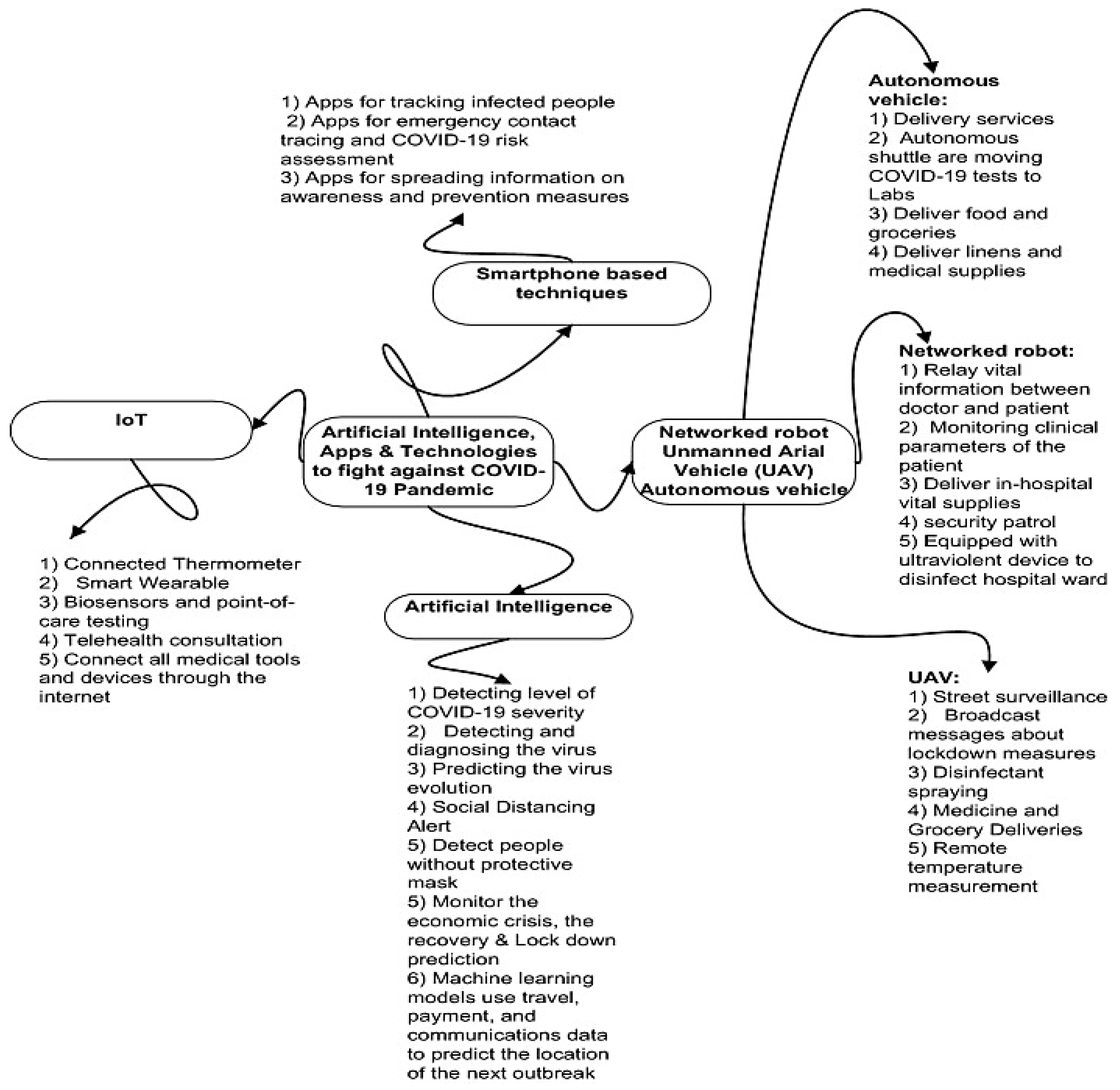AI can also predict the number of future COVID-19 cases by adequately analyzing the previous data on the infection [32]. Due to contextual conditions associated with COVID-19, innovative solutions were developed to ensure an appropriate function of day-to-day life. In research, the identified solutions offered the possibility to explore new technologies such as AI and IoT for better management of food delivery, temperature monitoring, virus monitoring and pandemic management while still following the government’s restrictions. Figure 1 depicts a detailed map of such approaches for evaluation, monitoring and prediction of COVID-19 impact.

The current research is focusing on the availability of simpler mathematical models to supply accurate predictions.

The main objective of this manuscript is to determine an integrated solution for modelling and simulation of the SARS-CoV-2 virus transmission process, on the Romanian territory. Currently, no solution is available that can be used to predict the main pandemic parameters evolution, with respect to the health system, both in relation to time and geographical position. Furthermore, another opportunity emerges due to the lack of a current method of pandemic control. The existence and simulation of a mathematical model for the virus transmission process would allow us to perform pandemic impact studies in Romanian society.

In this context, an important research aspect is the determination of the process’ mathematical model, meaning the determination of the multivariable functional relationship between all identified types of input signals (causes) and the relevant output signals (effects or results). The functional relationship will be a causal one, in the sense that an input signal modification will involve the modification of all corresponding output signals.

The dynamic process of transmitting the virus SARS-CoV-2, an evolution both, in relation to the time variable, and in terms of geographical position, is a process with distributed parameters; the final form of the proposed mathematical model should be expressed using techniques specific to this process type. The SARS-CoV-2 virus transmission is also a MIMO (Multiple Input Multiple Output) process, characterized by a large number of input signals (causes that influence the pandemic dynamics) and a large number of output signals (effects of input signals variation).

The input signals (causes or inputs) were grouped into three broad categories:

• Controllable input signals in the sense that their modification involves the modification of the output signals and these can be modified by various decisions (actions) of the involved decision makers, assumed for slowing down the pandemic spread;
• Uncontrollable input signals in the sense that their modification involves modification of the output signals, but their value, although variable, cannot be changed or cannot be changed significantly through decisions (actions) of the involved decision makers (practically, the values of these signals represent facts);
• Disturbance signals (which are also input signals as their modification involves the alteration of the output signals, influencing the pandemic’s spread in a negative way by increasing its speed).

Output signals (effects or outputs) are changed in value due to all mentioned input signals (at one point in time, a single input signal, several input signals, or all input signals at the same time may vary). In this context, the model of the SARS-CoV-2 virus transmission process, in relation to time, must be designed and parameterized to make the mathematical functional connection between all input signals and all output signals.

The first stage in the elaboration of this mathematical model is the mathematical quantification of each input signal’s influence on the output signals, considering that the mathematical model will run effective mathematical values. This stage is an essential one making possible the effective mathematical modelling of the process.

A strong aspect of the proposed solution’s overall impact is the determination of a mathematical model of the SARS-CoV-2 virus transmission specific to the Romanian territory, a model faithful to reality, with simulation availability. In this sense, due to the model’s proposed architecture flexibility, the model can be built gradually starting from a minimum number of input signals and, gradually, adding the effects of new input signals. Due to its flexibility, the model can be generalized for other pandemics or epidemics. The existence of such a mathematical model will have the following types of impact:

• Economic impact by pandemic/epidemic parameters prediction (duration, aggression, new waves, peaks of each wave), adding opportunities for both the budget sector and private companies, to make decisions regarding subsequent actions and to differentiate various forecasts, based on simulations results;
• Social impact by predicting the parameters of the pandemic materialized both by forecasting the time needed to resume the pre-pandemic population lifestyle and also forecasting this transition process stages; by knowing the parameters of the pandemic and based on the simulations results, the social impact reduction is materialized through the authorities possibilities to decide measures for the population protection, including the risk groups.

The first section is an introductive one. In the second section, the “experimental” data processed for the model identification are presented. Additionally, the main explanations associated with the input signals used for the modelling and their impact on the spreading of the COVID-19 virus.

In the third section, the types of mathematical models used for modelling the pandemic dynamics are described together with the corresponding equations, advantages and disadvantages of using each model for such a biomedical system.

In the fourth section, the simulation and the results interpretations of the proposed model are made. Additionally, the validity of the proposed model in the prediction of future evolutions of the pandemic is proven.

In the last section, the conclusions are drawn and some future research directions that will be approached are presented.

2. Data Processing for Model Identification

The data containing all the necessary information needed for model identification were received both from the authorities involved in combating the pandemic spread, from the infectious diseases hospitals and from profile research institutes (The Clinical Hospital of Infectious Diseases, Alessandrescu Rusescu National Institute for Mother and Child Health). The data between 28 February 2020 and 30 September 2020 were collected each day, in every county of Romania and they were stored in a database.

After implementing this database, the containing data were processed for determining the mathematical model of the pandemic dynamics on Romanian territory in the following way:

• The data were analyzed, in order to verify to gaps possibility between the days and the information; the identified missing data from the database were later collected and, in the final form, the database was completed;
• The data were processed accordingly for each day; for example, in order to obtain the relevant data for the entire of Romania, the data from all counties were merged and processed (in the case of the temperature or humidity, the data processing refers to the computation of the arithmetic average);
• The consistent information was selected; at this stage, the inconsistencies from the database structure were filtered and eliminated; more exactly, the inconsistent information was replaced after a study with consistent information;
• The data were organized in such a manner as to be processed in the next steps; for example, groups of data from the database were extracted and arranged in vectorial or matrixial form.

After processing the data were split into two categories:

• Possible inputs by each date: number of taken tests, inside temperature (in closed spaces such as supermarkets, offices, and rooms), outside temperature (in open spaces), outside humidity, quantified values of COVID-19 measures taken by the authorities in order to slow the pandemic spread;
• Possible outputs by each date: number of new cases, number of new deaths, total number of cases, total number of deaths.

In

Table 1. Examples of input data.

Date	Inside Temperature (°C)	Outside Temperature (°C)	Humidity (%)	No. of Tests	Quantified Value of COVID-19 Measures (%)
28 February 2020	21 °C	10.714 °C	72.286%	8	0%
28 March 2020	20.5 °C	16.571 °C	68.857%	86	86.85%
28 April 2020	19 °C	22.857 °C	71.571%	759	87%
28 May 2020	21.8 °C	28 °C	71.286%	1271	73%
28 June 2020	20.3 °C	32.429 °C	65.714%	1689	47.5%
28 July 2020	18.8 °C	33.571 °C	61.714%	2374	49.5%
28 August 2020	20.7 °C	34 °C	60%	3498	45.5%
28 September 2020	19.9 °C	25 °C	64%	4632	31.5%

and

Table 2. Examples of output data.

Date	No. of New Cases	No. of New Deaths	Total No. of Cases	Total No. of Deaths
28 February 2020	2	0	3	0
28 March 2020	160	5	1452	29
28 April 2020	277	19	11,616	650
28 May 2020	197	10	18,791	1229
28 June 2020	291	23	26,313	1612
28 July 2020	1151	33	47,053	2239
28 August 2020	1318	48	84,468	3507
28 September 2020	1271	30	123,944	4748

, some examples of data groups from the database structure are presented. There, only a part of the available data types for one day, in each month, is exemplified. Obviously, these data are available for the entire considered period.

In Table 1, the data associated with input signals are exemplified and, in Table 2, the data are associated with output signals. As a remark, the elaborated database contains much more data types (for example, the available drugs from the hospitals, medical available equipment from hospitals, and medical information regarding the patient).

Several studies indicate that the transmission of COVID-19 is affected by temperature [34]. In this context, an inverse correlation was found between the outside temperature and the daily number of infections. Other studies determine the temperature range for this effect. For instance, the virus transmission is hindered by a specific humidity above 6 g/kg and an average air temperature above 11 °C.

In some studies, the temperature is expressed as the average daily temperature or the average temperature over a time period. Others use average temperatures (an average between the minimum and the maximum recorded temperatures) [35], underlying that those countries, from a total of 204 considered, having high temperatures, showed fewer infections.

Recently, there have been several attempts to correlate temperature and humidity with the seasonality of the COVID-19 infection rate [36]. However, temperature and humidity are not the only factors that affect the seasonal virus infection rate.

Additionally, climate data are recorded outdoors, whereas most virus transmission is considered to occur indoors, which can have different conditions than the outside environment due to: heating, ventilation and air-conditioning (HVAC). The indoor conditions are affected by the socioeconomic status of the sample population and the geometric location of the country as well [37].

The main points in preventing the spread in society are hand hygiene, social distancing and quarantine. With increased testing capacity, detecting more COVID-19-positive patients in the community also enables the secondary case number reduction with stricter quarantine rules. Social distancing is advised, particularly in locations that have community transmission. Romanian authorities have installed quarantine and social/physical distancing as measures to prevent the further spread of the virus.

As an essential aspect of this research, the measures taken by the authorities with the purpose of lowering the COVID-19 pandemic spread were quantified based on the impact of the legislation existing on each date from the considered time interval over the population’s freedom of movement and socializing. The mentioned quantified values are enclosed between 0% and 100%.

The number of tests is also essential for pandemic dynamics. However, the processing of this signal is difficult due to the testing decrease during the weekends.

Using the daily gathered data, oscillations can appear on the data representation graphic due to the consistent differences between the number of tests taken during the working days and the number of tests taken during the weekend. The mentioned oscillations, in almost all cases, represent an impediment in the process identification of the mathematical models, an aspect which implies a deficit in the accuracy of the determined mathematical model. To address this issue, the effect of the oscillations is reduced by applying the 3-day average. This procedure will be useful in our future research based on Artificial Intelligence (AI) techniques. In order not to distort the original dynamics of the experimental responses, the averaging procedure was not extended for more than 3 days.

3. Types of Mathematical Models Used

In this manuscript, the transfer functions from the structure of a Multiple Input Single Output (MISO) mathematical model are identified using pairs of input–output data which were filtered as presented in the previous section. The estimation of a non-minimal order transfer function under a selection of oversimplified assumptions, such as constant variance errors, known order, and delays, is a prevalent strategy in the approaches now in use for the identification of MISO systems. Identifying the order of the transfer function which connects each input signal with each output signal is a difficult task due to the complexity of the approached biological process, the transmission of SARS-CoV-2 virus.

The process structure is presented in Figure 2, in the form of a black-box representation, where ${\mathrm{u}}_{\mathrm{i}}$(t) represents the input signals (i ∈ {1,…,5}) and y(t) represents the output signal.

The five input signals are the following:

• Inside temperature, ${\mathrm{u}}_1\left(\mathrm{t}\right)$;
• Outside temperature, ${\mathrm{u}}_2\left(\mathrm{t}\right)$;
• Humidity, ${\mathrm{u}}_3\left(\mathrm{t}\right)$;
• Number of tests taken each day, ${\mathrm{u}}_4\left(\mathrm{t}\right)$;
• Quantified value of COVID-19 measures taken by the authorities to limit the spread of the COVID-19 pandemic, ${\mathrm{u}}_5\left(\mathrm{t}\right)$.

Between each input signal and the output signal (daily number of cases or daily number of deaths), the corresponding transfer functions are determined.

A mathematical model of a dynamic system is defined as a collection of equations that accurately or reasonably describe the dynamics of the system. It should be noted that the dynamics of a particular system can be modelled using a corresponding particular mathematical model. From one system to another one, the model can have different parameters and structures; furthermore, a system can be represented in a variety of ways, resulting in a multitude of mathematical models.

3.1. Transfer Function Model

Transfer functions are often utilized in control theory to characterize the input–output dependencies in the case of linear time-invariant systems (these types of systems can be modelled in the time domain using ordinary differential equations with constant coefficients) [38]. The dependency between the input signal and the output signal written in the complex domain in the case of a SISO system (Single Input Single Output) is presented in (1):

$$\mathrm{Y}\left(\mathrm{s}\right)=\frac{\mathrm{n}\mathrm{u}\mathrm{m}\left(\mathrm{s}\right)}{\mathrm{d}\mathrm{e}\mathrm{n}\left(\mathrm{s}\right)}\mathrm{U}\left(\mathrm{s}\right)+\mathrm{E}(\mathrm{s}),$$

(1)

where: Y(s), U(s), and E(s) represent the Laplace transforms of the output signal, input signal and noise signal, respectively; num(s) and den(s) represent the numerator and the denominator of the transfer function which mathematically connects the U(s) and Y(s) signals; and num(s) and den(s) represent polynomials of “s” complex variable associated to the Laplace transform.

A linear time-invariant system [39] is considered, it is modelled by the following differential Equation (2):

$${\mathrm{a}}_0\mathrm{y}\left(\mathrm{t}\right)+{\mathrm{a}}_1\frac{\mathrm{d}}{\mathrm{d}\mathrm{t}}\mathrm{y}\left(\mathrm{t}\right)+\dots +{\mathrm{a}}_{\mathrm{n}-1}\frac{{\mathrm{d}}^{\mathrm{n}-1}}{{\mathrm{d}\mathrm{t}}^{\mathrm{n}-1}}\mathrm{y}\left(\mathrm{t}\right)+{\mathrm{a}}_{\mathrm{n}}\frac{{\mathrm{d}}^{\mathrm{n}}}{{\mathrm{d}\mathrm{t}}^{\mathrm{n}}}\mathrm{y}\left(\mathrm{t}\right)={\mathrm{b}}_0\mathrm{x}\left(\mathrm{t}\right)+{\mathrm{b}}_1\frac{\mathrm{d}}{\mathrm{d}\mathrm{t}}\mathrm{x}\left(\mathrm{t}\right)+\dots +{\mathrm{b}}_{\mathrm{m}-1}\frac{{\mathrm{d}}^{\mathrm{m}-1}}{{\mathrm{d}\mathrm{t}}^{\mathrm{m}-1}}\mathrm{x}\left(\mathrm{t}\right)+{\mathrm{b}}_{\mathrm{m}}\frac{{\mathrm{d}}^{\mathrm{m}}}{{\mathrm{d}\mathrm{t}}^{\mathrm{m}}}\mathrm{x}\left(\mathrm{t}\right),$$

(2)

where y is the output signal of the system and x is the input signal.

In (2), the ${\mathrm{a}}_{\mathrm{i}}$ (i $\in \{1,2,\dots ..,\mathrm{n}\}$) and ${\mathrm{b}}_{\mathrm{j}}$ (j $\in \{1,2,\dots ..,\mathrm{m}\}$), coefficients are constant. Consequently, the differential equation presented in (1) can be used for describing the operation of a linear system. Due to the fact that in (1), only one input signal and only one output signal occur, this type of differential equation can be used for modelling a SISO (Single Input Single Output) system.

By applying the Laplace transform for zero initial conditions to (1), it results in (3):

$$\mathrm{H}\left(\mathrm{s}\right)=\frac{\mathrm{Y}\left(\mathrm{s}\right)}{\mathrm{X}\left(\mathrm{s}\right)}=\frac{{\mathrm{b}}_{\mathrm{m}}·{\mathrm{s}}^{\mathrm{m}}+{\mathrm{b}}_{\mathrm{m}-1}·{\mathrm{s}}^{\mathrm{m}-1}\cdots \cdots \cdots +{\mathrm{b}}_1·\mathrm{s}+{\mathrm{b}}_0}{{\mathrm{a}}_{\mathrm{n}}·{\mathrm{s}}^{\mathrm{n}}+{\mathrm{b}}_{\mathrm{n}-1}·{\mathrm{s}}^{\mathrm{n}-1}\cdots \cdots \cdots +{\mathrm{a}}_1·\mathrm{s}+{\mathrm{a}}_0},$$

(3)

where $\mathrm{Y}\left(\mathrm{s}\right)=\mathrm{L}\left[\mathrm{y}\left(\mathrm{t}\right)\right]$ and $\mathrm{X}\left(\mathrm{s}\right)=\mathrm{L}\left[\mathrm{x}\left(\mathrm{t}\right)\right]$ represent the Laplace transforms of the output, with respect to the input signal, and $\mathrm{H}\left(\mathrm{s}\right)$ represents the transfer function of the modelled system. A system is practically feasible (practically implementable) only if $\mathrm{n}\ge \mathrm{m}$. If $\mathrm{n}>\mathrm{m}$ the system is strictly proper (the case of the majority of practically feasible systems); if $\mathrm{n}=\mathrm{m}$ the system is proper. The main advantage of applying the Laplace transform is the conversion of the differential Equation (2) (in the time domain) into an algebraic equation (in the complex domain), an equation which is further much simple to be mathematically processed.

The considered biological system (process) of the SARS-CoV-2 transmission dynamics is a MIMO one (Multiple Input Multiple Output) due to its complexity and due to the multitude of factors which influence it. However, in order to obtain a higher accuracy for the proposed mathematical models, the SARS-CoV-2 transmission process is modelled as a family of MISO (Multiple Input Single Output) models. More exactly, the cumulative effect of all the input signals to each output signal is modelled separately.

The general linear differential equation usable for modelling a MISO system with 5 input signals and one output signal is presented in (4):

$${\sum }_{\mathrm{i}=0}^{\mathrm{n}}{\mathrm{a}}_{\mathrm{i}}·\frac{{\mathrm{d}}^{\mathrm{i}}\left(\mathrm{y}\left(\mathrm{t}\right)\right)}{\mathrm{d}{\mathrm{t}}^{\mathrm{i}}}={\sum }_{\mathrm{j}=0}^{{\mathrm{m}}_1}{\mathrm{b}}_{1\mathrm{j}}·\frac{{\mathrm{d}}^{\mathrm{j}}\left({\mathrm{x}}_1\left(\mathrm{t}\right)\right)}{\mathrm{d}{\mathrm{t}}^{\mathrm{j}}}+{\sum }_{\mathrm{k}=0}^{{\mathrm{m}}_2}{\mathrm{b}}_{2\mathrm{k}}·\frac{{\mathrm{d}}^{\mathrm{k}}\left({\mathrm{x}}_2\left(\mathrm{t}\right)\right)}{\mathrm{d}{\mathrm{t}}^{\mathrm{k}}}+{\sum }_{\mathrm{p}=0}^{{\mathrm{m}}_3}{\mathrm{b}}_{3\mathrm{p}}·\frac{{\mathrm{d}}^{\mathrm{p}}\left({\mathrm{x}}_3\left(\mathrm{t}\right)\right)}{\mathrm{d}{\mathrm{t}}^{\mathrm{p}}}+{\sum }_{\mathrm{c}=0}^{{\mathrm{m}}_4}{\mathrm{b}}_{4\mathrm{c}}·\frac{{\mathrm{d}}^{\mathrm{c}}\left({\mathrm{x}}_4\left(\mathrm{t}\right)\right)}{\mathrm{d}{\mathrm{t}}^{\mathrm{c}}}+{\sum }_{\mathrm{c}=0}^{{\mathrm{m}}_5}{\mathrm{b}}_{5\mathrm{e}}·\frac{{\mathrm{d}}^{\mathrm{e}}\left({\mathrm{x}}_5\left(\mathrm{t}\right)\right)}{\mathrm{d}{\mathrm{t}}^{\mathrm{e}}},$$

(4)

where $\mathrm{y}\left(\mathrm{t}\right)$ is the output signal and ${\mathrm{x}}_1\left(\mathrm{t}\right)$, ${\mathrm{x}}_2\left(\mathrm{t}\right)$, ${\mathrm{x}}_3\left(\mathrm{t}\right)$, ${\mathrm{x}}_4\left(\mathrm{t}\right)$ and ${\mathrm{x}}_5\left(\mathrm{t}\right)$ are the input signals. In order for the system to be practically feasible, the following conditions: $\mathrm{n}\ge {\mathrm{m}}_1$, $\mathrm{n}\ge {\mathrm{m}}_2$, $\mathrm{n}\ge {\mathrm{m}}_3$, $\mathrm{n}\ge {\mathrm{m}}_4$ and $\mathrm{n}\ge {\mathrm{m}}_5$ have to be simultaneously accomplished. By applying to (4) the Laplace transform for zero initial conditions, the following equation results:

$$\begin{array}{cc}\hfill \left({\displaystyle \sum _{\mathrm{i}=0}^{\mathrm{n}}}{\mathrm{a}}_{\mathrm{i}}·{\mathrm{s}}^{\mathrm{i}}\right)·\mathrm{Y}\left(\mathrm{s}\right)& \hfill =\left({\displaystyle \sum _{\mathrm{j}=0}^{{\mathrm{m}}_1}}{\mathrm{b}}_{1\mathrm{j}}·{\mathrm{s}}^{\mathrm{j}}\right)·{\mathrm{X}}_1\left(\mathrm{s}\right)+\left({\displaystyle \sum _{\mathrm{k}=0}^{{\mathrm{m}}_2}}{\mathrm{b}}_{2\mathrm{k}}·{\mathrm{s}}^{\mathrm{k}}\right)·{\mathrm{X}}_2\left(\mathrm{s}\right)+\left({\displaystyle \sum _{\mathrm{p}=0}^{{\mathrm{m}}_3}}{\mathrm{b}}_{3\mathrm{p}}·{\mathrm{s}}^{\mathrm{p}}\right)·{\mathrm{X}}_3\left(\mathrm{s}\right)+\left({\displaystyle \sum _{\mathrm{c}=0}^{{\mathrm{m}}_4}}{\mathrm{b}}_{4\mathrm{c}}·{\mathrm{s}}^{\mathrm{c}}\right)·{\mathrm{X}}_4\left(\mathrm{s}\right)\\ \hspace{1em}& +\left({\displaystyle \sum _{\mathrm{e}=0}^{{\mathrm{m}}_5}}{\mathrm{b}}_{5\mathrm{e}}·{\mathrm{s}}^{\mathrm{e}}\right)·{\mathrm{X}}_5\left(\mathrm{s}\right),\hfill \end{array}$$

(5)

From (5), the output signal equation results:

$$\mathrm{Y}\left(\mathrm{s}\right)=\frac{\sum _{\mathrm{j}=0}^{{\mathrm{m}}_1}{\mathrm{b}}_{1\mathrm{j}}·{\mathrm{s}}^{\mathrm{j}}}{\sum _{\mathrm{i}=0}^{\mathrm{n}}{\mathrm{a}}_{\mathrm{i}}·{\mathrm{s}}^{\mathrm{i}}}·{\mathrm{X}}_1\left(\mathrm{s}\right)+\frac{\sum _{\mathrm{k}=0}^{{\mathrm{m}}_2}{\mathrm{b}}_{2\mathrm{k}}·{\mathrm{s}}^{\mathrm{k}}}{\sum _{\mathrm{i}=0}^{\mathrm{n}}{\mathrm{a}}_{\mathrm{i}}·{\mathrm{s}}^{\mathrm{i}}}·{\mathrm{X}}_2\left(\mathrm{s}\right)+\frac{\sum _{\mathrm{p}=0}^{{\mathrm{m}}_3}{\mathrm{b}}_{3\mathrm{p}}·{\mathrm{s}}^{\mathrm{p}}}{\sum _{\mathrm{i}=0}^{\mathrm{n}}{\mathrm{a}}_{\mathrm{i}}·{\mathrm{s}}^{\mathrm{i}}}·{\mathrm{X}}_3\left(\mathrm{s}\right)+\frac{\sum _{\mathrm{c}=0}^{{\mathrm{m}}_4}{\mathrm{b}}_{4\mathrm{c}}·{\mathrm{s}}^{\mathrm{c}}}{\sum _{\mathrm{i}=0}^{\mathrm{n}}{\mathrm{a}}_{\mathrm{i}}·{\mathrm{s}}^{\mathrm{i}}}·{\mathrm{X}}_4\left(\mathrm{s}\right)+\frac{\sum _{\mathrm{e}=0}^{{\mathrm{m}}_5}{\mathrm{b}}_{5\mathrm{e}}·{\mathrm{s}}^{\mathrm{e}}}{\sum _{\mathrm{i}=0}^{\mathrm{n}}{\mathrm{a}}_{\mathrm{i}}·{\mathrm{s}}^{\mathrm{i}}}·{\mathrm{X}}_5\left(\mathrm{s}\right),$$

(6)

In (6), the following notations are made:

$${\mathrm{H}}_1\left(\mathrm{s}\right)=\frac{\sum _{\mathrm{j}=0}^{{\mathrm{m}}_1}{\mathrm{b}}_{1\mathrm{j}}·{\mathrm{s}}^{\mathrm{j}}}{\sum _{\mathrm{i}=0}^{\mathrm{n}}{\mathrm{a}}_{\mathrm{i}}·{\mathrm{s}}^{\mathrm{i}}},$$

(7)

$${\mathrm{H}}_2\left(\mathrm{s}\right)=\frac{\sum _{\mathrm{k}=0}^{{\mathrm{m}}_2}{\mathrm{b}}_{2\mathrm{k}}·{\mathrm{s}}^{\mathrm{k}}}{\sum _{\mathrm{i}=0}^{\mathrm{n}}{\mathrm{a}}_{\mathrm{i}}·{\mathrm{s}}^{\mathrm{i}}},$$

(8)

$${\mathrm{H}}_3\left(\mathrm{s}\right)=\frac{\sum _{\mathrm{p}=0}^{{\mathrm{m}}_3}{\mathrm{b}}_{3\mathrm{p}}·{\mathrm{s}}^{\mathrm{p}}}{\sum _{\mathrm{i}=0}^{\mathrm{n}}{\mathrm{a}}_{\mathrm{i}}·{\mathrm{s}}^{\mathrm{i}}},$$

(9)

$${\mathrm{H}}_4\left(\mathrm{s}\right)=\frac{\sum _{\mathrm{c}=0}^{{\mathrm{m}}_4}{\mathrm{b}}_{4\mathrm{c}}·{\mathrm{s}}^{\mathrm{c}}}{\sum _{\mathrm{i}=0}^{\mathrm{n}}{\mathrm{a}}_{\mathrm{i}}·{\mathrm{s}}^{\mathrm{i}}},$$

(10)

$${\mathrm{H}}_5\left(\mathrm{s}\right)=\frac{\sum _{\mathrm{e}=0}^{{\mathrm{m}}_5}{\mathrm{b}}_{5\mathrm{e}}·{\mathrm{s}}^{\mathrm{e}}}{\sum _{\mathrm{i}=0}^{\mathrm{n}}{\mathrm{a}}_{\mathrm{i}}·{\mathrm{s}}^{\mathrm{i}}},$$

(11)

The ${\mathrm{H}}_{\mathrm{f}}\left(\mathrm{s}\right)$ (f $\in \{1,2,3,4,5\}$) notation is referring to the transfer function which mathematically connects the ${\mathrm{X}}_{\mathrm{f}}\left(\mathrm{s}\right)$ input signal with the $\mathrm{Y}\left(\mathrm{s}\right)$ output signal.

Considering these notations, (6) can be rewritten under the form:

$$\mathrm{Y}\left(\mathrm{s}\right)={\mathrm{H}}_1\left(\mathrm{s}\right)·{\mathrm{X}}_1\left(\mathrm{s}\right)+{\mathrm{H}}_2\left(\mathrm{s}\right)·{\mathrm{X}}_2\left(\mathrm{s}\right)+{\mathrm{H}}_3\left(\mathrm{s}\right)·{\mathrm{X}}_3\left(\mathrm{s}\right)+{\mathrm{H}}_4\left(\mathrm{s}\right)·{\mathrm{X}}_4\left(\mathrm{s}\right)+{\mathrm{H}}_5\left(\mathrm{s}\right)·{\mathrm{X}}_5\left(\mathrm{s}\right),$$

(12)

Furthermore, (12) can be rewritten in the vector form, as:

$$\mathcal{Ƴ}=\mathcal{H}·\mathcal{X},$$

(13)

where the output vector, is:

$$\mathrm{Ƴ}=\mathrm{Y}\left(\mathrm{s}\right),$$

(14)

and the input vector, is:

$$\mathcal{X}=\left(\begin{array}{c}{\mathrm{X}}_1\left(\mathrm{s}\right)\\ \begin{array}{c}{\mathrm{X}}_2\left(\mathrm{s}\right)\\ {\mathrm{X}}_3\left(\mathrm{s}\right)\\ {\mathrm{X}}_4\left(\mathrm{s}\right)\end{array}\\ {\mathrm{X}}_5\left(\mathrm{s}\right)\end{array}\right)$$

(15)

In (13),

$$\mathcal{H}=\left(\begin{array}{ccc}{\mathrm{H}}_1\left(\mathrm{s}\right)& \begin{array}{ccc}{\mathrm{H}}_2\left(\mathrm{s}\right)& {\mathrm{H}}_3\left(\mathrm{s}\right)& {\mathrm{H}}_4\left(\mathrm{s}\right)\end{array}& {\mathrm{H}}_5\left(\mathrm{s}\right)\end{array}\right)$$

(16)

represents the transfer vector of the MISO model, more exactly, the mathematical model of the considered process.

3.2. ARX Model and ARMAX Model

The ARX (autoregressive-exogenous) model is the most basic model that includes the input signal. As it is the outcome of solving linear regression equations in analytic form, the estimation of the ARX model is the most efficient of the polynomial estimation methods. As a result, the ARX model is preferable, especially when the model order is large.

The ARX (n, m) model is defined in (17):

$$\mathrm{y}\left(\mathrm{k}\right)={\mathrm{a}}_1\mathrm{y}\left(\mathrm{k}-1\right)+{\mathrm{a}}_2\mathrm{y}\left(\mathrm{k}-2\right)+\dots +{\mathrm{a}}_{\mathrm{n}}\mathrm{y}\left(\mathrm{k}-\mathrm{n}\right)+{\mathrm{b}}_1\mathrm{u}\left(\mathrm{k}-1\right)+{\mathrm{b}}_2\mathrm{u}\left(\mathrm{k}-2\right)+{\mathrm{b}}_{\mathrm{m}}\mathrm{u}\left(\mathrm{k}-\mathrm{m}\right)+\mathrm{v}\left(\mathrm{k}\right)$$

(17)

where y is the model output signal; u is the model input signal; ${\mathrm{a}}_{\mathrm{i}}$ is the ${\mathrm{i}}^{\mathrm{t}\mathrm{h}}$ autoregressive (AR) parameter; ${\mathrm{b}}_{\mathrm{i}}$ is the ${\mathrm{i}}^{\mathrm{t}\mathrm{h}}$ exogenous (X) parameter; and v is the noise.

When the system’s disturbance v(k) is not white noise, the connection between the deterministic and stochastic dynamics might decrease the quality of the ARX model estimation. To reduce the error, the model order has to be set higher than the system order, especially when the signal-to-noise ratio is low. However, raising the model order might alter several dynamic properties of the model, such as its stability.

ARMAX (autoregressive-moving-average) models are frequently utilized in system identification because they accurately capture a wide range of real-world processes with a minimal level of complexity. ARMAX models have the same stochastic context as Kalman filtering and are a common tool in control engineering for both, system model and control design.

ARMAX models are part of the equation-error model family. Their result is given as the sum of three regression terms including historical inputs, outputs, and white noise samples. The parallel connection of a deterministic component is driven by the observed input signal u(t) and of a stochastic part driven by a remote white noise v(t).

The deterministic part is represented by the discrete transfer function B(${\mathrm{z}}^{-1}$)/A(${\mathrm{z}}^{-1}$) and its output signal y(t) is not available. The stochastic part is denoted by the discrete transfer function C(${\mathrm{z}}^{-1}$)/A(${\mathrm{z}}^{-1}$) and its output signal is a white noise v(t) that can be the effect of non-accessible disturbances on the state of the deterministic part.

Before estimating a model, it is necessary to select an appropriate model structure. The model structure is chosen based on an understanding of the physical systems. In system identification, three types of models are commonly used: black-box models, grey-box models, and user-defined models. The black-box model states that systems are unknown and that all model parameters may be adjusted without regard, for the physical environment. To change randomly all the settings is not allowed. The grey-box model states that some of the underlying dynamical or physical characteristics are known and that the model parameters may be constrained in some way. The user-defined model is based on the assumption that the frequently used parametric models cannot accurately reflect the model that has to be estimated.

To aid in the modelling of an unknown system, several parametric model structures are available. Differential equations and transfer functions are used to explain systems in metric models. These models give insight into the mechanics of the system as well as compact model architectures. To test a variety of architectures to choose the optimal one is frequently advantageous. A parametric model structure is a black-box model that specifies either a continuous-time or discrete-time system.

In particular, the technique described is based on the extension of the dynamic Frisch scheme. Once a high-order ARX model has been identified, the polynomials A(${\mathrm{z}}^{-1}$), B(${\mathrm{z}}^{-1}$) are estimated by using the properties of polynomials with common factors. Finally, part C(${\mathrm{z}}^{-1}$) is estimated by considering the relation with its high-order autoregressive approximation.

In Figure 3, the ARMAX model is presented and its equation is described by the relation (18):

$$\mathrm{A}\left({\mathrm{z}}^{-1}\right)\mathrm{y}\left(\mathrm{t}\right)=\mathrm{B}\left({\mathrm{z}}^{-1}\right)\mathrm{u}\left(\mathrm{t}\right)+\mathrm{C}\left({\mathrm{z}}^{-1}\right)\mathrm{v}\left(\mathrm{t}\right),$$

(18)

where:

$$\mathrm{A}\left({\mathrm{z}}^{-1}\right)=1+{\mathrm{a}}_1{\mathrm{z}}^{-1}+\cdots +{\mathrm{a}}_{{\mathrm{n}}_{\mathrm{a}}}{\mathrm{z}}^{-{\mathrm{n}}_{\mathrm{a}}},$$

(19)

$$\mathrm{B}\left({\mathrm{z}}^{-1}\right)={\mathrm{b}}_0+{\mathrm{b}}_1{\mathrm{z}}^{-1}+\cdots +{\mathrm{b}}_{{\mathrm{n}}_{\mathrm{b}}}{\mathrm{z}}^{-{\mathrm{n}}_{\mathrm{b}}},$$

(20)

$$\mathrm{C}\left({\mathrm{z}}^{-1}\right)=1+{\mathrm{c}}_1{\mathrm{z}}^{-1}+\cdots +{\mathrm{c}}_{{\mathrm{n}}_{\mathrm{c}}}{\mathrm{z}}^{-{\mathrm{n}}_{\mathrm{c}}},$$

(21)

are polynomials depending on the delay operators ${\mathrm{z}}^{-1}$ (i.e., ${\mathrm{z}}^{-1}$x(t) = x(t − 1)).

Figure 4 depicts the technique for modelling a dynamical system using the identification approach, both in the ARX and ARMAX models.

Reviewing the technique for the identification strategy is usually beneficial. Four main processes are involved in building the model using extracted data as highlighted in Figure 4:

• Data set acquisition;
• A collection of candidate models and selecting the best model from the set;
• Model’s parameter estimation;
• The validation of the proposed model.

The data set is an important component of the identification method:

• The dataset collection process is establishing which signals to be measured and when to measure them;
• The goal of the experiment design is to make these decisions; in this study, data were recorded and gatheed from a hospital system over a period of time;
• The input and output datasets were separated into two parts; the first section was selected for the estimation part and the second for the validation part.

The selection of the candidate models and the determination of the best model in the set:

• Selecting an appropriate model structure is required before estimating its parameters; the black-box model states that the identified system is unknown and all the model parameters have to be adjusted without taking into account the physical context;
• A parametric model structure is a black-box model that models either a continuous-time or discrete-time system; the concept of parametric model-based system identification is to derive a mathematical model guided by real-world data.

Model’s parameter estimation:

• Estimating linear models using a specific model structure and exploring which model structure best fits the data (different configuration was used and the best configuration result is declared as the identification solution);
• If the simple model structures do not produce good models, there can be selected more complex model structures by specifying a higher model order for the same linear model structure; a higher model order increases the model flexibility for capturing complex phenomena; however, an unnecessarily high order can make the model less reliable.

The ARX model’s structure may be represented in the form of Equation (22), and the overall structure of the MISO system which is described in this manuscript for all the five input signals, the ARX model is shown in Equation (23).

$$\mathrm{A}\left({\mathrm{z}}^{-1}\right)\mathrm{y}\left(\mathrm{t}\right)=\mathrm{B}\left({\mathrm{z}}^{-1}\right)\mathrm{u}\left(\mathrm{t}\right)+\mathrm{v}\left(\mathrm{t}\right),$$

(22)

$$\mathrm{A}\left({\mathrm{z}}^{-1}\right)\mathrm{y}\left(\mathrm{t}\right)={\mathrm{B}}_1\left({\mathrm{z}}^{-1}\right){\mathrm{u}}_1\left(\mathrm{t}\right)+{\mathrm{B}}_2\left({\mathrm{z}}^{-1}\right){\mathrm{u}}_2\left(\mathrm{t}\right)+{\mathrm{B}}_3\left({\mathrm{z}}^{-1}\right){\mathrm{u}}_3\left(\mathrm{t}\right)+{\mathrm{B}}_4\left({\mathrm{z}}^{-1}\right){\mathrm{u}}_4\left(\mathrm{t}\right)+{\mathrm{B}}_5\left({\mathrm{z}}^{-1}\right){\mathrm{u}}_5\left(\mathrm{t}\right)+\mathrm{v}\left(\mathrm{t}\right),$$

(23)

The ARMAX model structure is similar to the ARX structure, but it includes an additional component that reflects the moving average error. When dominating disturbances that have entered early in the process, ARMAX modes are beneficial. The ARMAX model’s structure may be represented in the form of Equation (24) and the overall structure of the MISO ARMAX model is indicated in the equation:

$$\mathrm{A}\left({\mathrm{z}}^{-1}\right)\mathrm{y}\left(\mathrm{t}\right)={\mathrm{B}}_1\left({\mathrm{z}}^{-1}\right){\mathrm{u}}_1\left(\mathrm{t}\right)+{\mathrm{B}}_2\left({\mathrm{z}}^{-1}\right){\mathrm{u}}_2\left(\mathrm{t}\right)+{\mathrm{B}}_3\left({\mathrm{z}}^{-1}\right){\mathrm{u}}_3\left(\mathrm{t}\right)+{\mathrm{B}}_4\left({\mathrm{z}}^{-1}\right){\mathrm{u}}_4\left(\mathrm{t}\right)+{\mathrm{B}}_5\left({\mathrm{z}}^{-1}\right){\mathrm{u}}_5\left(\mathrm{t}\right)+\mathrm{C}\left({\mathrm{z}}^{-1}\right)\mathrm{v}\left(\mathrm{t}\right),$$

(24)

4. Prediction of Future Pandemic Evolution

The infectious nature of the disease and lack of vaccinations created a restriction on social interactions and economic collapse, overwhelming economic and healthcare systems everywhere. These effects created an urgent need to study the virus, predict the spread, find a cure, and help local authorities all over the world to decide the required measures for virus spread prevention. The need is more obvious for helping countries to decide the best time to open back their economies and manage healthcare logistics.

To predict—with accuracy and specificity—the spread of COVID-19 is important. Using the existing data, there is a need to forecast trends in the virus expansion. Many governments rely heavily on such predictions to plan their next actions, related to medical resources allocation or to lockdowns level required shifts (to ease or to increase).

Considering that this virus has made impossible the focus on a single mode of transmission, to concentrate on various factors that can affect the spread of the disease became fundamentally important, for scientific communities.

Most models assume a uniformly distributed population with the same levels of immunity or susceptibility to infection and a relatively immobile population. However, the modern world does not always follow all these conditions. For example, populations are clustered, people of different ages and economic conditions have different susceptibilities to diseases, public opinion adds to the dangers of contagion shift over time, and the population is extremely mobile.

Populations are more mobile, concentrated, and social, making it difficult to model epidemics as flows. Instead, modern models use diffusion equations and complexity equations to represent the spread of a contagion. Moreover, these models are much more data-driven because conditions change. For example, social distancing, patterns of mobility, and nonuniform mixing affect the contagion, causing it to surge in some places and die out in other places, which can only be represented in the data.

4.1. Identification Model

4.1.1. Continuous Transfer Function Model

The next five equations were determined based on real data collected through the National Committee for Special Emergency Situations, as follows:

$${\mathrm{H}}_1\left(\mathrm{s}\right)=\frac{0.08897\mathrm{s}-0.0003917}{{\mathrm{s}}^4+0.7874{\mathrm{s}}^3+0.01296{\mathrm{s}}^2+0.0003136\mathrm{s}+1.395·{10}^{-5}},$$

(25)

$${\mathrm{H}}_2\left(\mathrm{s}\right)=\frac{0.0087\mathrm{s}+7.098·{10}^{-5}}{{\mathrm{s}}^4+0.004978{\mathrm{s}}^3+0.01069{\mathrm{s}}^2+2.571·{10}^{-5}\mathrm{s}+1.345·{10}^{-5}},$$

(26)

$${\mathrm{H}}_3\left(\mathrm{s}\right)=\frac{-0.004716\mathrm{s}+9.113·{10}^{-5}}{{\mathrm{s}}^4+0.01741{\mathrm{s}}^3+0.0108{\mathrm{s}}^2+0.0001057\mathrm{s}+2.951·{10}^{-6}}$$

(27)

$${\mathrm{H}}_4\left(\mathrm{s}\right)=\frac{-0.0009913\mathrm{s}+5.405·{10}^{-5}}{{\mathrm{s}}^4+0.01583{\mathrm{s}}^3+0.01108{\mathrm{s}}^2+8.476·{10}^{-5}\mathrm{s}+7.494·{10}^{-6}}$$

(28)

$${\mathrm{H}}_5\left(\mathrm{s}\right)=\frac{-0.0003472\mathrm{s}-8.991·{10}^{-5}}{{\mathrm{s}}^4+0.04924{\mathrm{s}}^3+0.02067{\mathrm{s}}^2+0.0003081\mathrm{s}+5.897·{10}^{-5}}$$

(29)

The significance of the transfer functions is:

• ${\mathrm{H}}_1\left(\mathrm{s}\right)$—transfer function correlating inside temperatures with the number of new cases.
• ${\mathrm{H}}_2\left(\mathrm{s}\right)$—transfer function correlating outside temperatures with the number of new cases.
• ${\mathrm{H}}_3\left(\mathrm{s}\right)$—transfer function correlating humidity with the number of new cases.
• ${\mathrm{H}}_4\left(\mathrm{s}\right)$—transfer function correlating number of tests with the number of new cases.
• ${\mathrm{H}}_5\left(\mathrm{s}\right)$—transfer function correlating quantified values of COVID-19 measures with the number of new cases.

Each of these transfer functions provides relevant distinct information between a specific input affecting the spread of the disease and the outcome, the number of new cases.

4.1.2. ARX Model

The following equations provide a detailed specification of the ARX model parameters.

The discrete-time ARX model is represented in the following form (30) and the vectorial form (31):

$${\mathrm{A}}_1·{\mathrm{Z}}_{11}·\mathrm{y}\left(\mathrm{t}\right)=\mathrm{U}\left(\mathrm{t}\right)·\left({\mathrm{B}}_1{·\mathrm{Z}}_{12}\right)+\mathrm{e}\left(\mathrm{t}\right),$$

(30)

where:

$$\begin{gathered} {\mathrm{A}}_1=\left(\begin{array}{ccccc}1& -1.196& 0.02204& 0.09766& 0.07964\end{array}\right), \\ {\mathrm{B}}_1=\left(\begin{array}{cccccccc}0.9044& -1.362& 2.713& -4.543& 5.256& -3.663& 1.049& -0.07813\\ 0.02698& -2.851& 3.611& 0.5376& -3.477& 2.163& -0.02327& -0.2289\\ 0& 0& 0& 0& 0& 0& 6.863& 0\\ 3.769& 18.38& -37.44& 7.828& 3.77& 19.77& -22.05& 7.033\\ 6.082& 5.736& -31.75& 17.2& 1.406& 10.02& -19.39& 8.294\end{array}\right) \\ \mathrm{U}\left(\mathrm{t}\right)=\left(\begin{array}{ccccc}{\mathrm{u}}_1\left(\mathrm{t}\right)& {\mathrm{u}}_2\left(\mathrm{t}\right)& {\mathrm{u}}_3\left(\mathrm{t}\right)& {\mathrm{u}}_4\left(\mathrm{t}\right)& {\mathrm{u}}_5\left(\mathrm{t}\right)\end{array}\right), \\ {\mathrm{Z}}_{11}=\left(\begin{array}{c}1\\ {\mathrm{z}}^{-1}\\ {\mathrm{z}}^{-2}\\ {\mathrm{z}}^{-3}\\ {\mathrm{z}}^{-4}\end{array}\right) \\ {\mathrm{Z}}_{12}=\left(\begin{array}{c}{\mathrm{z}}^{-1}\\ {\mathrm{z}}^{-2}\\ {\mathrm{z}}^{-3}\\ {\mathrm{z}}^{-4}\\ {\mathrm{z}}^{-5}\\ {\mathrm{z}}^{-6}\\ {\mathrm{z}}^{-7}\\ {\mathrm{z}}^{-8}\end{array}\right) \end{gathered}$$

(31)

4.1.3. ARMAX Model

The vector-matrix equation associated to the ARMAX model is given by (32) and the vectorial form is as in (33):

$${\mathrm{A}}_2·{\mathrm{Z}}_{21}·\mathrm{y}\left(\mathrm{t}\right)=\mathrm{U}\left(\mathrm{t}\right)·\left({\mathrm{B}}_2{·\mathrm{Z}}_{22}\right)+\mathrm{C}·{\mathrm{Z}}_{32}·\mathrm{e}\left(\mathrm{t}\right),$$

(32)

where:

$$\begin{gathered} {\mathrm{A}}_2=\left(\begin{array}{ccccc}1& -1.847& 1.306& -1.007& 0.528\end{array}0.0296-0.00126\right), \\ {\mathrm{B}}_2=\left(\begin{array}{ccccc}0& -0.0585& 1.97& -2.682& 0.8727\\ 0& -0.3194& -1.093& 2.999& -1.582\\ 0& 0.3429& 0.3429& 0.3429& 0.3429\\ 0& -4.382& 29.17& -46.42& 21.65\\ 0& 4.971& 4.565& -27.68& 17.65\end{array}\right) \\ \mathrm{C}=\left(\begin{array}{ccccc}1& -0.7708& 0.644& -0.8162& 0.1557\end{array}0.0686-0.2813\right) \\ {\mathrm{Z}}_{21}=\left(\begin{array}{c}1\\ {\mathrm{z}}^{-1}\\ {\mathrm{z}}^{-2}\\ {\mathrm{z}}^{-3}\\ {\mathrm{z}}^{-4}\\ {\mathrm{z}}^{-5}\\ {\mathrm{z}}^{-6}\end{array}\right) \\ {\mathrm{Z}}_{22}=\left(\begin{array}{c}1\\ {\mathrm{z}}^{-1}\\ {\mathrm{z}}^{-2}\\ {\mathrm{z}}^{-3}\\ {\mathrm{z}}^{-4}\end{array}\right) \\ {\mathrm{Z}}_{32}=\left(\begin{array}{c}1\\ {\mathrm{z}}^{-1}\\ {\mathrm{z}}^{-2}\\ {\mathrm{z}}^{-3}\\ {\mathrm{z}}^{-4}\\ {\mathrm{z}}^{-5}\\ {\mathrm{z}}^{-6}\end{array}\right) \end{gathered}$$

(33)

As a remark, the ARMAX model equations in comparison with the above presented ARX model equations contain additionally a six previous errors computation given by the C(z) vector.

4.2. Simulation Results

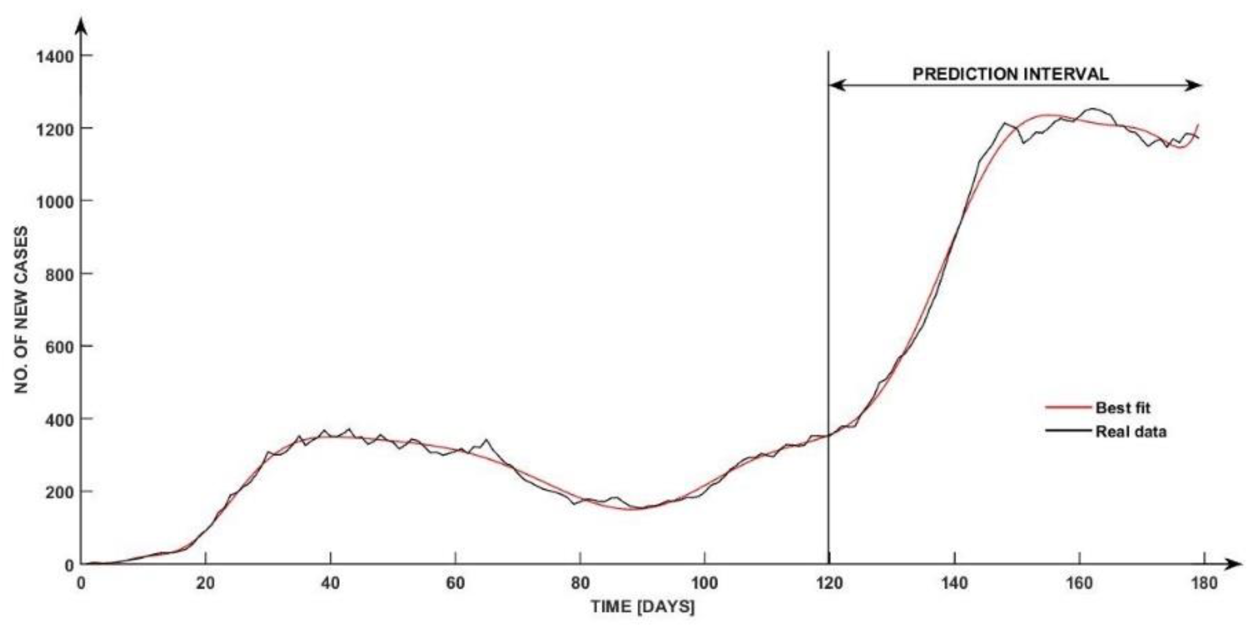
In Figure 5, the black curve provides a visual representation of the evolution of the number of new cases “experimentally determined” in relation to time.

The other five coloured curves represent responses of the proposed model, based on continuous transfer functions by applying at its inputs the same values as the “experimental ones” (for which the real number of cases was obtained). In this case, different variations of the number of poles and zeros for obtaining the best fit were chosen, to analyze an extended evaluation of the best solution.

As available below, the estimated curves follow the black curve (the real data curve) closely. The curves represent the evolution of the case numbers in 120 days. The following interval between $[121,180]$ days represents the prediction offered through the model of the continuous transfer vector (which contains as elements the transfer functions ${\mathrm{H}}_1\left(\mathrm{s}\right)$, ${\mathrm{H}}_2\left(\mathrm{s}\right)$, ${\mathrm{H}}_3\left(\mathrm{s}\right)$, ${\mathrm{H}}_4\left(\mathrm{s}\right)$ and ${\mathrm{H}}_5\left(\mathrm{s}\right)$).

The model performance is highlighted using the cumulated relative error in percentages defined by:

$$\mathrm{c}\mathrm{r}\mathrm{e}\mathrm{p}=100·\frac{\sum _{\mathrm{i}=1}^{\mathrm{N}}\left|{\mathrm{y}}_{\mathrm{s}\mathrm{i}\mathrm{m},\mathrm{k}}-{\mathrm{y}}_{\mathrm{r}\mathrm{k}}\right|}{\sum _{\mathrm{i}=1}^{\mathrm{N}}\left|{\mathrm{y}}_{\mathrm{r},\mathrm{k}}\right|}[\mathrm{\%}]$$

(34)

where: crep—the cumulative relative error (%), N—the number of the pairs of the considered data samples, ${\mathrm{y}}_{\mathrm{r},\mathrm{k}}$—the real value (the “experimental” value) of the considered output signal associated with the sample k and ${\mathrm{y}}_{\mathrm{s}\mathrm{i}\mathrm{m},\mathrm{k}}$—the simulated value of the output signal associated with the sample k, obtained through the simulation of one of the proposed mathematical models. Consequently, the fit between the two responses is given by:

$$\mathrm{f}\mathrm{i}\mathrm{t}=100\mathrm{\%}-\mathrm{c}\mathrm{r}\mathrm{e}\mathrm{p}$$

(35)

where the crep value is computed using the data corresponding to the considered responses.

The degrees of the polynomials of the numerators and of the denominators of the five transfer functions are centralized in

Table 3. The centralizer of the parameters associated with the continuous transfer functions.

The Curve	No. of Zeros for Each Transfer Function	No. of Poles for Each Transfer Function
Estimation_1	[1 1 1 1 1]	[4 4 3 3 3]
Estimation_2	[1 1 1 2 2]	[8 8 7 7 7]
Estimation_3	[1 2 1 1 2]	[4 4 3 3 3]
Estimation_4	[1 1 2 1 1]	[6 6 6 6 6]
Estimation_5	[2 2 2 2 2]	[6 5 5 4 4]

(these polynomials depend on the complex variable “s” associated with the Laplace transform).

In Figure 6, the best solution using Estimation_3 from Table 3 is depicted with a fit of 97.23%. The difference in obtaining a 100% fit is given by the inconsistency of data gathering due to the not optimal feedback provided through the national official platforms on weekends affecting the validation model as seen in the interval between day 135 and day 160. During this time interval, the graphic shows a few oscillations, but the estimated model does not, so this could be a natural outcome due to the inconsistency mentioned before.

The five coloured responses presented in Figure 7 are the responses of the proposed ARX models (with different parameters) in comparison with the “experimental response”. The simulations of the five proposed ARX models are made in the same conditions as the simulation presented in Figure 5.

In Figure 7, the errors are visible due to consistent distances (visible on several time domains) between the real curve and the estimated one. The ARX model estimation shows a slightly less performance than in the case of the continuous transfer function estimation which was detailed above.

As shown in Figure 8, the response of the best ARX model, with a fit equal to 89.42% is obtained using Estimation_2 from

Table 4. The centralizer of the polynomials orders for the ARX model.

The Curve	na	nb	nk
Estimation_1	[4 4 4 4 4]	[2 2 2 2 2]	[1 1 1 1 1]
Estimation_2	[4 4 4 4 4]	[1 1 1 1 1]	[1 1 1 1 1]
Estimation_3	[6 6 6 6 6]	[2 2 2 2 2]	[1 1 1 1 1]
Estimation_4	[8 8 8 6 6]	[1 1 1 2 2]	[1 1 1 1 1]
Estimation_5	[6 6 6 4 4]	[2 2 2 2 2]	[1 1 1 1 1]

and follows the experimental curve with visible higher deviations than in the case of the continuous transfer functions model. So far, the best solution is provided by the transfer functions model estimation.

In Figure 9, all five responses of the ARMAX models are available. The main difference consists of a larger estimation deviation for the last period (the last 20 days).

The best fit equal to 89.42% in this case is provided in Figure 10, using Estimation_5 from

Table 5. The centralizer of the polynomials orders for the ARMAX model.

The Curve	na	nb	nc	nk
Estimation_1	[4 4 4 4 4]	[2 2 2 2 2]	[2 2 2 2 2]	[1 1 1 1 1]
Estimation_2	[4 4 4 4 4]	[1 1 1 1 1]	[1 1 1 1 1]	[1 1 1 1 1]
Estimation_3	[6 6 6 6 6]	[2 2 2 2 2]	[2 2 2 2 2]	[1 1 1 1 1]
Estimation_4	[8 8 8 6 6]	[1 1 1 2 2]	[1 1 1 1 1]	[1 1 1 1 1]
Estimation_5	[6 6 6 4 4]	[2 2 2 2 2]	[2 2 2 2 2]	[1 1 1 1 1]

and it follows with acceptable accuracy the experimental curve.

In the case of new daily cases prediction, the most efficient method is the continuous transfer function.

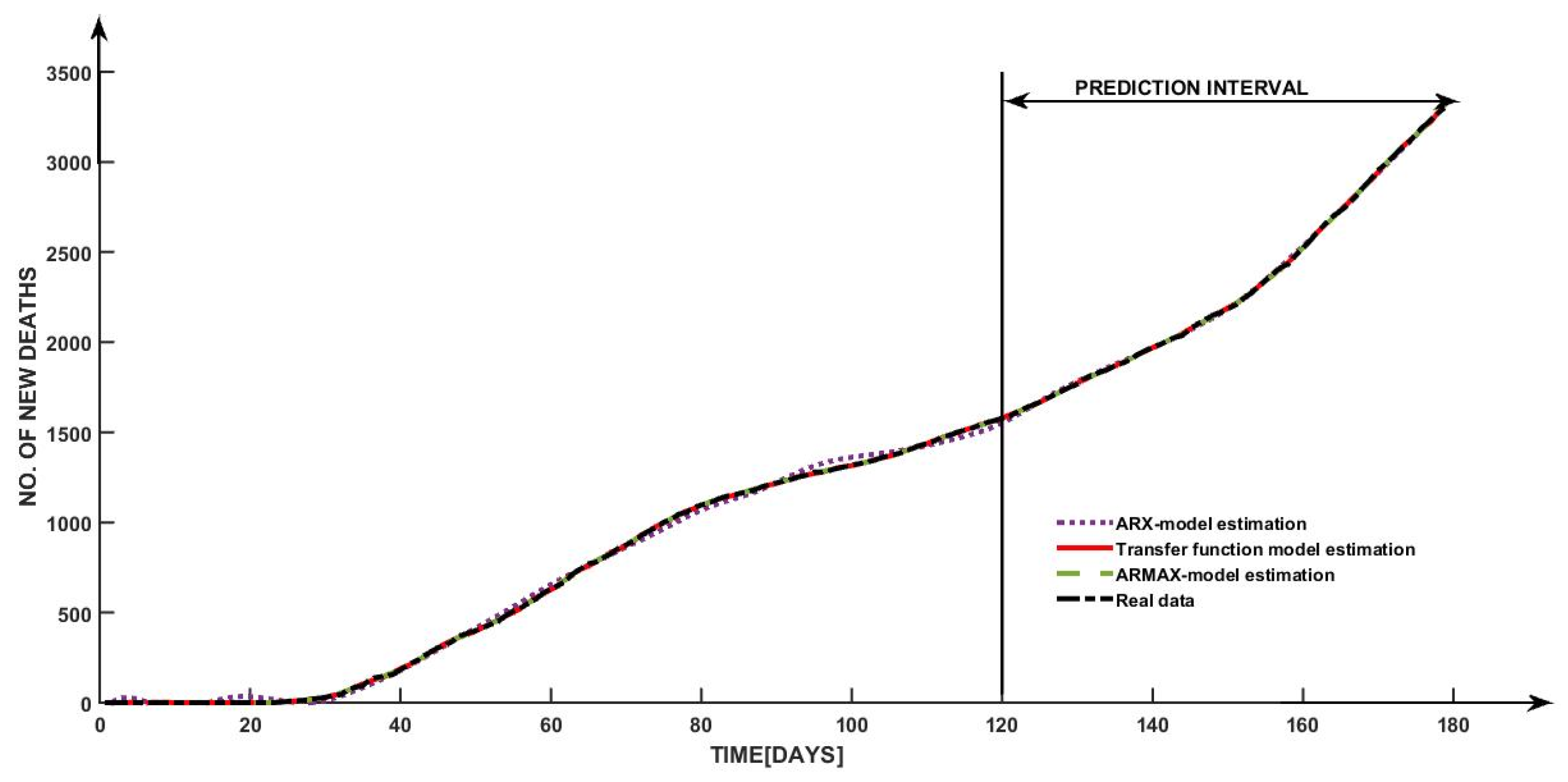
Furthermore, using the proposed types of models, the prediction of the future number of daily deaths can be estimated too.

In the case of this application, all three considered models proved to align very high accuracy over the experimental curve as it is highlighted in Figure 11, with a fit higher than 99.59%.

The visible superposition can be explained through a continuous constant increase in the number of deaths and independently of the number of cases.

5. Conclusions

The current research proposes three estimation mathematical models for SARS-CoV-2 virus transmission dynamics based on Romanian data collection. The parameters of the proposed dynamical models are identified using information collected by Romanian Healthcare Institutions (such as the Infectious Diseases Hospital, The National Committee for Special Emergency Situations, Research Institutes and County Health Departments). In order to obtain the best solution, three types of mathematical models were evaluated: transfer vector model with transfer functions as elements, ARX models and ARMAX models. The best solution was determined in the fourth section of this manuscript by comparing the fit values obtained after the simulation of all the proposed models. Furthermore, a study regarding the complexity of the proposed models is presented in the current research work. In this study, the data corresponding to the first 6 months of the pandemic in Romania were considered and they were split into two sets; the first one (containing the data for the first 4 months) was used for the estimation of the proposed models’ parameters and the second one (containing the data for the last 2 months), for testing the prediction capacity of the proposed models. The best fit was obtained for the transfer vector model (97.16%) and its associated simulations prove the efficiency of usage, in practice. The efficiency of the prediction horizon extension can be improved by considering a larger data set (associated with a longer period).

As mentioned before, the proposed MISO model, based on using the transfer function, generates the best performances.

As described in the introduction, in the literature, ARIMA models were utilized as well. In this context, in our research, we used ARMAX models (i.e., an ARIMA model with an exogenous variable). Consequently, they generate higher modelling performances.

From our perspective, the main advantage of the mathematical models proposed in the presented research in comparison with the SIR model is the fact that we have used experimental identification. Thus, we have processed the real data adding a significant impact for an accurate model determination. In the case of a relatively new virus such as COVID-19, with unappropriated monitoring for long and consistent periods of time, we consider that the analytical modelling (used for example in determining the SIR model) is disadvantageous with respect to the experimental one.

Obviously, AI-based techniques (for example, neural network usage) represent a consistent part of the future, in many domains, including mathematical modelling. However, in the case of dynamic systems with more input signals, the neural models have in general, a high complexity and they require, to be trained, significant computation power. Furthermore, in general, the neural nonlinear models generate better performances than the linear ones, an aspect which introduces supplementary problems in their numerical implementation.

In opposition, the proposed MISO model based on transfer functions is a linear one, very simple for numerical implementation. Furthermore, as a disadvantage in relation to the classical models, the neural networks present important limitations in the cases when the training signals are affected by disturbances and noises and when both, insufficient data and too many data are available. This situation is simpler to solve with classical modelling techniques.

The limitation of the prediction period of the currently proposed models is due to the fact that, in the first six months of the pandemic, the values of the considered signals (both inputs and outputs) were highly particular and they did not cover their entire domains of variation. Consequently, the longer the considered period is, the higher the consistency of the used “experimental” data is and implicitly higher the quality of the proposed models. By extending the considered period of time, only the accuracy is improved, but the used procedures are the same, the proposed solutions being general ones. In order not to increase without a justification the complexity of the proposed models, to approximate the dynamics of each output signal of interest a mathematical model of MISO type was determined. This procedure, due to the previous remark, is preferred over the case of considering only one more complex MIMO model.

Furthermore, the following development directions are identified:

• The extension of the period of time considered for collecting the data in order to improve the accuracy of the proposed models and to enlarge their prediction horizon;
• The consideration of a larger number of input and output signals;
• Extension of the models by considering, also, the pandemic geographical spread;
• The design of an appropriate control strategy to impose a certain nonaggressive dynamic for the pandemic based on the proposed models.

In the case of the last proposed future development direction, some starting points for future research are next presented. In Figure 12, a negative feedback control structure for controlling the dynamics of the interest output signal (which can be, for example, the number of new cases, the number of daily deaths or the number of persons hospitalized in intensive care) is proposed (${\mathrm{y}}_{\mathrm{r}\mathrm{e}\mathrm{f}}$(t) signifies the set-point signal for y(t) and e(t) signifies the error signal). However, in the real context, not all the signals can be varied by the human factor.

Considering the main human controllable signals, the mentioned control structure can be modified under the form depicted in Figure 13, where only control signals u₄(t) and u₅(t) are considered; u₁(t), u₂(t) and u₃(t) can be interpreted as exogenous input signals or even disturbances, in some values ranges. In the case of the negative feedback structure from Figure 13, the proposed model is used for the controller tuning.

In Figure 14, a control structure based on IMC (Internal Model Control) strategy is proposed. By using the proposed model, the equivalent deviation of the real process in comparison with the initial identified model is evaluated and its effect is rejected.

These proposed control strategies remain as developments for future research, in different scenarios, considering, also, the potential shifts in the progress of the virus spread.