Accurate Tracking Algorithm for Cluster Targets in Multispectral Infrared Images

Abstract

To address the issue of poor tracking accuracy and the low recognition rate for multiple small targets in infrared images caused by uneven image intensity, this paper proposes an accurate tracking algorithm based on optical flow estimation. The algorithm consists of several steps. Firstly, an infrared image subspace model is established. Secondly, a full convolutional network (FCN) is utilized for local double-threshold segmentation of the target image. Furthermore, a target observation model is established using SIR filtering particles. Lastly, a shift vector sum algorithm is employed to enhance the intensity of the infrared image at a certain time scale in accordance with the relationship between the pixel intensity and the temporal parameters of the detected image. Experimental results demonstrate that the multi-target tracking accuracy (MOTA) reaches 79.7% and that the inference speed frame per second (FPS) reaches 42.3. Moreover, the number of ID switches during tracking is 9.9% lower than that of the MOT algorithm, indicating high recognition of cluster small targets, stable tracking performance, and suitability for tracking weak small targets on the ground or in the air.

1. Introduction

The application of large numbers of drones forming drone swarms in the military, coupled with their increasing level of intelligence, has the potential to overturn the rules of future warfare. Drone swarms have the capability to accomplish complex tasks that are difficult to achieve with a single drone. However, the scale and complexity of drone swarms, resulting from the increase in the number of UAVs, also bring numerous security risks. These risks extend beyond mission-related factors and may pose a threat to national security and public safety. A swarm of UAVs represents one example of clusters of weak targets with distinct characteristics; thus, detecting, identifying, and tracking such clusters has become a technical challenge [1]. Among the challenges faced in this field are the low signal-to-noise ratio imaging of cluster weak targets in complex environments, where they tend to be submerged in complex backgrounds. Moreover, the uneven intensity of IR images further diminishes the recognition rates and tracking accuracy of multiple small targets [2]. Consequently, achieving fine target tracking in infrared images has become a pressing technical challenge. To address this challenge, this paper presents research on an accurate multi-target tracking algorithm for infrared images based on optical flow estimation. This algorithm aims to solve the problem of accurate tracking and recognition rates for weak and small targets in infrared image clusters.

There are various problems in computer vision, including motion target recognition. However, image tracking techniques face challenges due to factors such as the complex uncertainty of the environment, background, and target, which can cause motion targets to become blurred and jittery during tracking. Moreover, when the target is far away from the detection system, it may appear as a point target or point source target, making it difficult to detect and recognize due to the lack of spatial information, such as shape, size, dimension, and texture, as well as the similarity in motion characteristics between the target and decoy. This can lead to the loss or mistracking of the target. At the two moments of temperature change between day and night, the target cannot be detected or tracked due to the zero difference in radiation temperature between the target and the background [3]. To address these challenges, various studies propose different solutions. Reference [4] suggests enhancing feature extraction by increasing the degree of learning of edge features and using adaptive updating to determine the need for model updates in tracking filtered targets. However, the threshold-setting judgment of this method requires extensive experience and significantly affects the accuracy of the results. On the other hand, reference [5] presents a fast multi-domain convolutional neural network tracking algorithm that improves tracking accuracy by synthesizing features from multi-channel video. Nonetheless, this approach leads to increased processing time and poor real-time performance. In contrast, reference [6] introduces a multi-layer depth linear feature interpolation approach for training depth models through feature fusion. However, obtaining the depth model for this algorithm from a large number of image training sets is computationally intensive and time-consuming. In reference [7], a multi-layer convolutional feature-based method is proposed to calculate the correlation of multiple targets in a video image, which is then used for adaptive decision fusion in tracking. However, this algorithm requires combining the history information of multiple trackers and is computationally complex. Lastly, reference [8] proposes an improved RTMD Net tracking algorithm that divides multi-channel video images into different grid scales to enhance tracking accuracy. However, the formation of grid-scale information is complex and poses difficulties in information management.

This paper proposes research on an accurate multi-target tracking algorithm for infrared images based on optical flow estimation, which improves the accuracy and recognition rate of infrared image multi-target tracking. The algorithm is suitable for rapid multi-target identification, detection, and tracking. Infrared target detection and tracking systems are passive detection systems with the advantages of good concealment, strong anti-interference capability, high accuracy, and good performance [9,10]. They have become some of the indispensable key technologies in modern warfare. The algorithm can be applied to target detection and tracking of threatening infrared targets (UAVs, missiles, aircraft, etc.) in the air [11], at sea, and on land, and to provide target-related information for defensive weapons systems [12], which has certain research significance and value.

This paper is divided into five parts. Firstly, in this introduction, the current state of research on related technologies has been analyzed. An infrared multi-target precision tracking algorithm has been proposed to address current technical problems, such as the poor accuracy and low recognition rate of infrared multi-target tracking, and its application environment and related research significance and value have been clearly defined. This is followed by a brief introduction to the underlying theory of this research in the Section 2. The theoretical derivation and algorithmic structure of the algorithm proposed in this paper are discussed in detail in the Section 3. The experimental validation and detailed data analysis are then carried out in the Section 4. The strengths and weaknesses of the algorithm proposed in this paper are discussed in light of the data analysis, and future directions for continued research and the application of the technique are explored. Finally, clear conclusions and the significance and value of the research are outlined in the Section 5.

2. Related Work

2.1. Fully Convolutional Neural Networks (FCNs)

A fully convolutional neural network (FCN) [13] is a network model based on deep learning, which is widely used in image segmentation. FCNs have the following advantages:

(1)

The full connection layer is replaced with a convolution layer to achieve end-to-end convolution network training.

(2)

To achieve pixel-level segmentation, all pixel features in the image are classified by prediction. However, for an image with a complicated visual environment, the FCN network still adopts the simplest deconvolution method, which results in blurred contours and serious adhesion of the segmented image.

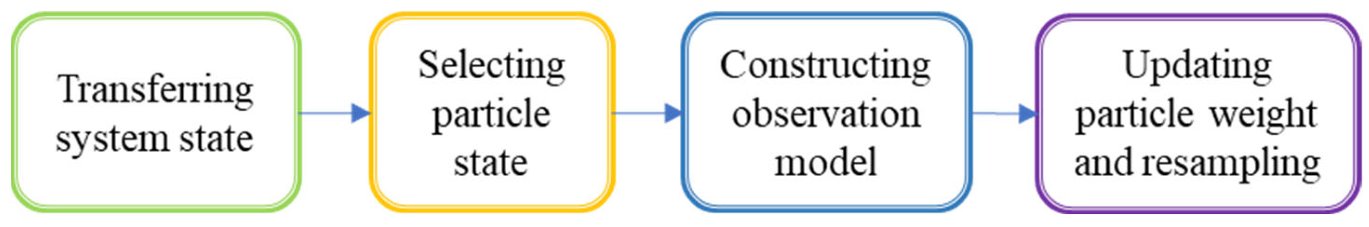
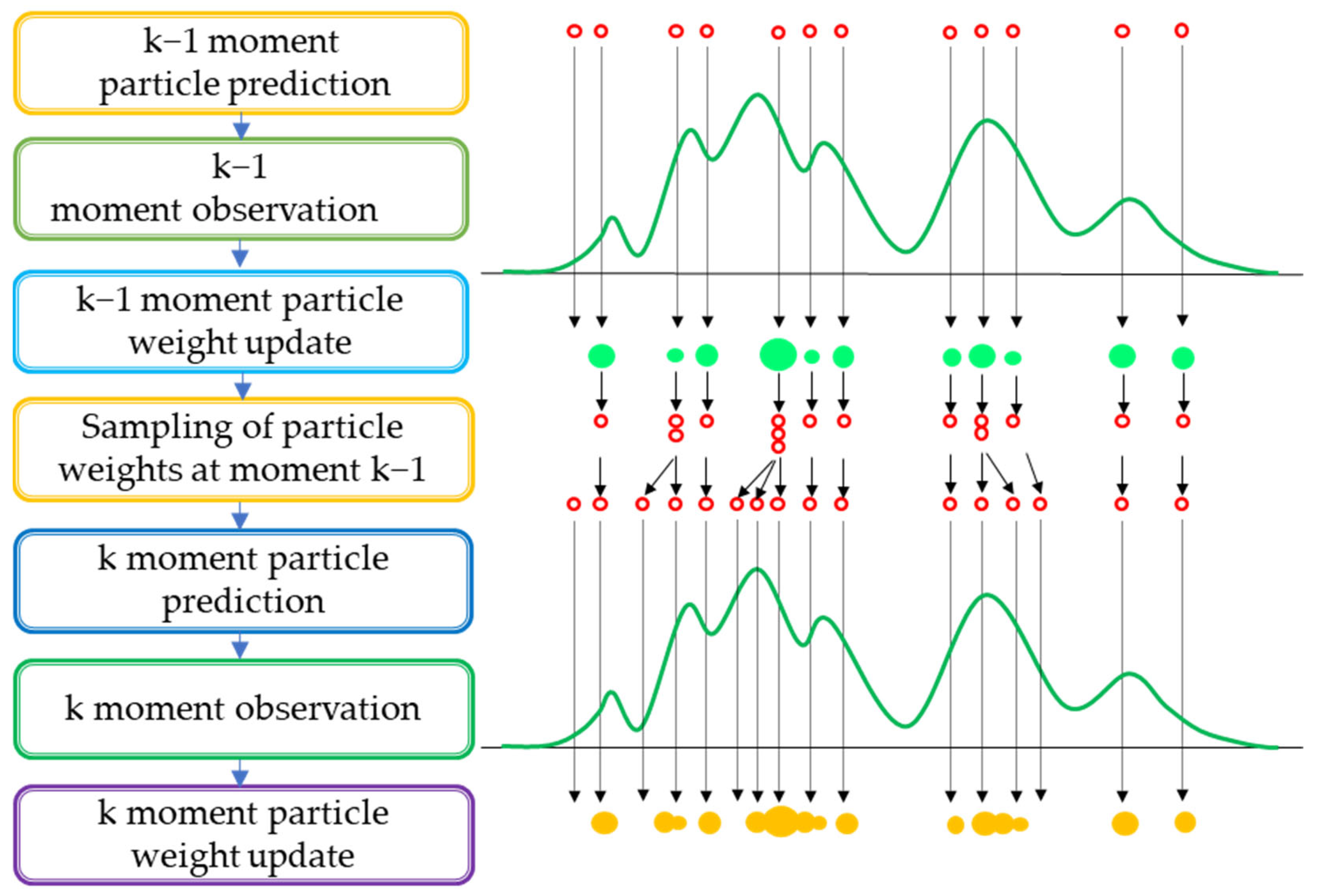
2.2. Particle Filter

The idea of particle filtering is based on the Monte Carlo method, which uses sets of particles to represent probabilities of things and can be used for any form of state-space model. The core idea is to express the distribution through random state particles drawn from posterior probabilities through a sequential importance sampling method. In simple terms, particle filtering is the process of approximating a probability density function by finding a set of random samples propagated in a state space and replacing the integration operation with the sample mean to obtain the state minimum variance distribution.

Although the probability distribution of the algorithm is only an approximation of the true distribution, it is unaffected by the constraint according to which random quantities must satisfy a Gaussian distribution when solving non-linear filtering problems due to its non-parametric nature, and it can express a wider range of distributions than a Gaussian model, in addition to having a greater ability to model the non-linear properties of the variable parameters. Thus, particle filtering can more accurately express the posterior probability distribution based on the observed and control quantities and can be used to solve SLAM problems. New variants of the MCMC have been developed as improvement strategies for particle filters, unscented particle filters, Rao–Blackwellized particle filters, and Gaussian particle filters.

2.3. Thermal Radiation Analysis

The long-wave infrared data in the dataset were acquired in April when the outdoor temperature was about 15 °C, the surface temperature of a moving car was roughly 30 °C to 40 °C, and the temperature of a boat in a river was about 20 °C to 30 °C.

$$M(T,\lambda )=\frac{2\pi h{c}^2}{{\lambda }^5(\exp (\frac{ch}{k\lambda T})-1)}$$

(1)

where $M(T,\lambda )$ is the spectral radiance of the blackbody (${\mathrm{W}·\mathrm{m}}^{-2}{·\mathsf{\mu }\mathrm{m}}^{-1}$), $\lambda$ is the wavelength of radiation (μm), T is the absolute blackbody temperature (k, T = t + 273 k), C is the speed of light ($2.998\times {10}^8{\mathrm{ms}}^{-1}$), h is Planck’s constant ($3.626\times {10}^{-34}\mathrm{JS}$), and k is the Boltzmann constant.

According to the Wien’s law formula:

$${\lambda }_{\mathrm{m}}·T=2.898\times {10}^3(\mathsf{\mu }\mathrm{m}·\mathrm{K})$$

(2)

where ${\lambda }_{\mathrm{m}}$ is the wavelength at the maximum blackbody spectral radiation brightness (μm) and T is the absolute temperature of the blackbody (K).

According to Wien’s law, when the surface temperature of a driving car is 30 °C, the wavelength range can be found between 9.25 and 9.56 μm by heat radiation calculation. When the surface temperature of a boat in the river is 20 °C, the wavelength range is between 9.56 and 9.89 μm. The wavelength of the thermal radiation generated by the car and the boat in the river is between 8 and 14 μm. A long-wave infrared detector is used to obtain long-wave infrared image information of the target.

3. Methods

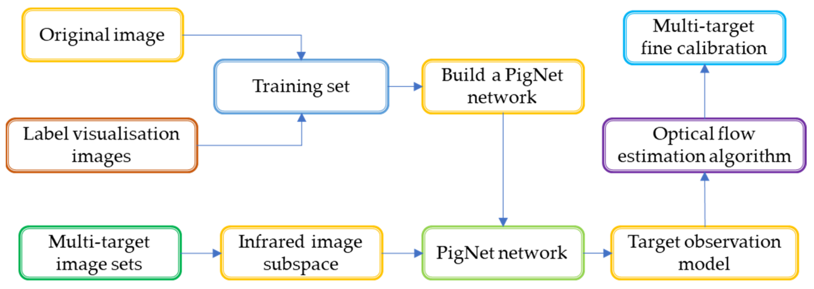
3.1. Establishment of an Infrared Image Subspace

An infrared image subspace is a complete linear aggregation of weak targets, and each feature node represents an image information parameter to be extracted. Considering the rigidity of infrared image extraction in complex environments, the larger the actual range of the subspace, the larger the total amount of matching information.

Assuming that the maximum range of variation of a weak target never exceeds the parameter $\lambda$ in an infrared image subspace and that the maximum information quantity condition of the extracted image is $r$, the infrared image subspace of the weak target can be defined as:

$$A={\displaystyle \underset{r=1}{\overset{n}{\int }}\frac{\lambda }{r({\delta }_1+{\delta }_2)}}dr$$

(3)

where $\lambda$ represents the number of weak target limits, $r=1$ represents the minimum extraction matching condition of the weak target feature node, $r=n$ represents the maximum extraction matching condition of the weak target feature node, and ${\delta }_1$ and ${\delta }_2$ represent two different infrared image information parameter values.

3.2. Local Segmentation of Double-Threshold Images

Mask R-CNN [14] is an instance segmentation algorithm, and the region of interest (ROI) is used as a network branch of the deep convolution neural network to realize the instance segmentation of the target image. To preserve the accuracy of the target spatial location coordinates, the Mask R-CNN network replaces the ROIPool operation with the ROIAlign operation. ROIAlign can be used to correct the misplaced layer of spatial quantization feature extraction. The bilinear difference keeps the spatial position accuracy between the input network and the output network constant and corresponds to the coordinate value of the ROI bin. The dependency between the judgment class (Class) and the output mask (MASK) is minimized, and the prediction of the binary mask, with the average binary cross-entropy loss for each target, is realized separately, which reduces the competitiveness among the classes and improves the efficiency of image segmentation.

Based on the Mask R-CNN network structure, the network depth and width are optimized, and transfer learning is carried out. The parameters and network model are obtained by calculating the segmentation accuracy of the different layers and different convolution cores.

Finally, the optimal network model is determined as a PigNet network structure, and two improvements to the Mask R-CNN network structure are made in terms of the convolution layer and class number:

(1)

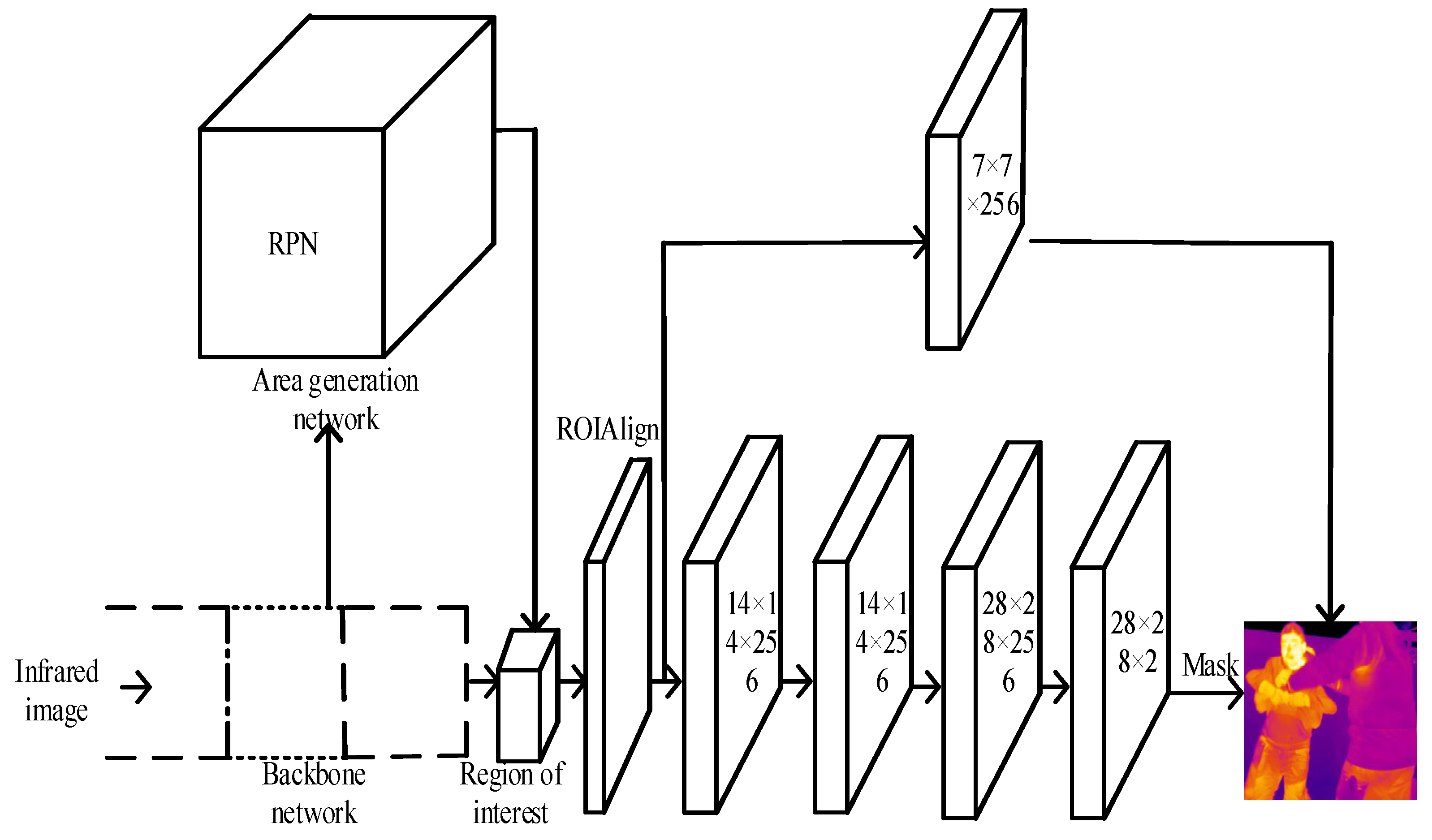
For different target regions in the image, the Mask R-CNN network is changed from 69 convolution layers to 12 layers in the fourth stage, which can reduce the level of feature loss and the amount of convolution computation.

(2)

The number of classes in the last convolution layer of the mask branch of the Mask R-CNN network is optimized and adjusted to the PigNet class and background class. The structure is shown in Figure 1.

A PigNet network structure [15] consists of 5 stages and 44 convolution layers. All convolution layers adopt a residual learning structure. Each arc consists of 3 convolution layers, and 1 × 1 × 64 layers represent convolution layers with a 1 × 1 convolution nucleus and 64 channels. The residual learning structure reduces the number of parameters to a great extent, which simplifies the calculation and keeps the spatial position accuracy of the target unchanged. Through the arc part of the network diagram, the residual learning structure transmits the input information directly to the following layers and also partially reduces the feature loss [16]. The residual learning structure can also reduce the sliding step size of each convolution layer from 2 pixels to 1/4 while increasing the number of output channels to 2048.

In the structure of the PigNet backbone network, two kinds of feature extraction processes are involved: on the one hand, the network model 4 conv12 convolution layer output map is analyzed and processed through the candidate region network (RPN), and the required feature information is extracted; on the other hand, it propagates forward to generate the feature map. RPN can then quickly select regions of interest.

The loss function ($F$) of the PigNet network is mainly composed of three parts: classification error ($F_s$), detection error ($F_b$), and segmentation error ($F_k$). The formula is as follows:

$$F=F_s+F_b+F_k$$

(4)

In Formula (4), $F_s$ and $F_b$ represent the processing of the fully connected layer that is used to predict the regression box coordinates of the category and the target space for all the areas of interest. $F_k$ represents segmentation and assigns a mask to the target image for each area of interest. To calculate the loss function of region segmentation, only the relative entropy error of the pig class can be taken into account. To avoid competition between classes, the relative entropy error of the pig class is calculated without considering the background class. The main function of $F_b$ is to ensure that the coordinates of the object image’s regression box do not deviate. $F_k$ is used to ensure the accuracy of the target image generation mask. The class branch predicts that the ROI is a pig class so that $F_k$ only needs to predict the pixels of the pig class. The contour of the target image is distinct, and no conglutination occurs, thus ensuring the accuracy of the contour position coordinate information at different depths and that the image can achieve accurate segmentation.

In this paper, the PigNet network model is used to calculate 2 regions of interest by convolution. $F_b$ is used to predict the position coordinates of the regression box in the target space, and $F_k$ is used to predict the position coordinates of the regression box in the target space to form a binary mask by combining the mean binary cross-entropy loss function with the sigmoid function [17]. The segmented image is represented as two different color masks, which are placed at two different layer depths. Even if there are more images of the segmented object, the PigNet model forms a corresponding binary mask for each segmented object.

3.3. Construction of the Target Observation Model

Firstly, the SIR filter particle method [18] is used to construct the target observation model. The concrete steps include the selection of the particle state, the transfer of the system state, the construction of the observation model, the updating of the particle weight, and resampling. The operation steps are shown in Figure 2.

In the composition-building step of the SIR filter algorithm, one first selects the important probability function as:

$$\mathrm{q}(x_k^{(i)}|x_{k-1}^{(i)},y_k)=p(x_k^{(i)}|x_{k-1}^{(i)})$$

(5)

Then, based on the particle weights:

$$M_k^{(i)}\propto M_{k-1}^{(i)}·\frac{p(y_k|x_k^{(i)})·p(x_k^{(i)}|x_{k-1}^{(i)})}{\mathrm{q}(x_k^{(i)}|x_{k-1}^{(i)},y_k)}=p(y_k|x_k^{(i)})·M_{k-1}^{(i)}$$

(6)

After resampling, again:

$$M_{k-1}^{(i)}=\frac{1}{N}$$

(7)

Finally, by simplification:

$$M_{k-1}^{(i)}\propto p(y_k|x_k^{(i)})$$

(8)

This step realizes the theoretical derivation of the particle filtering algorithm. Here, $M_k^{(i)}$ and $M_{k-1}^{(i)}$ represent the k moments, k − 1 represents the particle weights, $x_k$ represents the observed variable at moment k, $y_k$ represents the state at moment k, $p(y_k|x_{1:k})$ represents the posterior probability, $q(y|x)$ represents the proposed distribution, and N represents the N samples sampled from the posterior probabilities.

First, one selects the particle state using the following formula:

$$W_k=\left(x,y,s\right)$$

(9)

where $\left(x,y\right)$ represents the coordinates of the particles in the infrared image, that is, the center position of the particle rectangle; $s$ represents the scale factor of the rectangle; and $W_k$ represents the particle state. A total of 200 particles are selected from the SIR-filtered particles, and the selected particles are initialized and restored to their initial position at the center of the target frame. That is:

$$W_0=\left(x_0,y_0,s_0\right)$$

(10)

where $\left(x_0,y_0\right)$ represents the initial position of the center of the target box and $s_0$ represents the scale factor of the initial change in the rectangular box.

One initializes the particle scale to 1 and constructs the HSV color histogram of the initial position target box [19].

Then, the state of the system is transferred: the particle position is transferred from the previous frame to the next frame using the autoregressive second-order transfer model [20]. The autoregressive second-order transfer model randomly combines the previous particle states and predicts the particle position in the next frame based on the combined results. The specific expressions of the autoregressive second-order transfer model are as follows:

$$X_k-\overline{X}=A_1\left(X_{k-1}-\overline{X}\right)+A_2\left(X_{k-2}-\overline{X}\right)+R·z$$

(11)

where ${\mathrm{X}}_k$ represents the corresponding particle state at the time $k$; $\overline{X}$ represents the estimated mean value of all the particles; $X_{k-1}$ represents the corresponding particle state at the time $k-1$; $X_{k-2}$ represents the corresponding particle state at the time $k-2$; $z$ stands for random noise; $A_1$ and $A_2$ are a pair of constants; and R represents the specific propagation radius of the particle.

Then, one predicts the specific state of particles at the time $k$ according to the above formula:

$$W_k=\frac{A_1\left(W_{k-1}-\overline{X}\right)+A_2\left(W_{k-2}-\overline{X}\right)}{\overline{X}}+R\cdot z_k$$

(12)

where $z_k$ represents the noise at the time $k$. The process is shown in Figure 3.

Then, we construct the observation model. After the particle position prediction in the next frame, we must observe the particles to judge the actual similarity between the target and the real state. If the actual similarity is high, it will be given a larger weight, and vice versa. Firstly, using the HSV color region histogram $\widehat{p}(x)$ representing $x$, the candidate particle, and $\widehat{q}$, the HSV color region histogram representing the target reference model, the Pap distance coefficient between them is:

$$\Re \left[\widehat{p}(w),\widehat{q}\right]={\displaystyle \sum _{v=1}^n({\widehat{p}}_v(w){\widehat{q}}_v)}$$

(13)

where $\Re$ represents the Babbitt distance coefficient between $\widehat{p}(w)$ and $\widehat{q}$; $v$ represents the specific dimension of the vector; ${\widehat{p}}_v(w)$ represents the HSV color region histogram of the candidate particle $w$ under the $v$-dimensional vector; and ${\widehat{q}}_v$ represents the HSV color region histogram of the target reference model under the $v$-dimensional vector.

The observation model is constructed by defining the actual measurement distribution of two HSV color region histograms, as shown in the following formula:

$$\left\{\begin{array}{l}\frac{\left[\widehat{p}(w),\widehat{q}\right]}{\chi }=\Re \left[\widehat{p}(w),\widehat{q}\right]\\ p\left(w_k\left|x_k\right.\right)\infty \exp \left(\gamma \right)\end{array}\right.$$

(14)

where $\chi$ represents the actual measured distribution of two HSV color regions, $p\left(w_k\left|x_k\right.\right)$ represents the observation model, $\lambda$ represents the observation threshold, and $\gamma$ usually has a value of 20.

Additionally, we update the weight of particles in the observation model. The update algorithm is as follows:

$${\displaystyle \sum _{i=1}^N{w}_{k+1}^i=1}$$

(15)

where $N$ represents the total number of particles; $i$ represents the update threshold; and $w_{k+1}^i$ represents a particle in the observation model, which satisfies:

$$w_{k+1}^i\infty p\left(w_k\left|x_{{}_k}^i\right.\right)$$

(16)

where $p\left(w_k\left|x_{{}_k}^i\right.\right)$ represents the updated observation model.

Then, the target box corresponding to the maximum weight particle is taken as the final position of the target box.

Finally, resampling is performed. The particles are sorted in descending order according to the weight of the particles. When the total number of particles is fixed, the total number of particles with larger weights is increased, the total number of particles with smaller weights is decreased, or the particles with smaller weights may even be dropped.

3.4. Target Analysis and Tracking of Infrared Dim and Small Images Based on the Optical Flow Estimation Model

This paper uses an optical flow estimation model to analyze dim and small targets in infrared images. According to the relationship between the pixel strength and time parameter of the detected image, the intensity of the infrared image is set at a certain time scale using the moving vector algorithm [21]. At a given time, the intensity value can be expressed as follows:

$$U(x,y)=H(x,y,t)$$

(17)

where $H(x,y,t)$ represents the intensity of the pixels at the time $t$, and $x$ and $y$ represent the positions of the pixels. Assuming that the pixels of the infrared image increase within the fixed period $\Delta t$ of the infrared image, the pixels can be represented as follows:

$$H(x+\Delta x,y+\Delta y,\Delta t)=\frac{\partial U}{\partial t}(\Delta x+\Delta y+\Delta t)$$

(18)

In the above calculation formula, the meaning of each parameter remains unchanged.

By synthesizing the numerical relationship between the two pixels, the numerical relationship before and after the change in the pixels can be calculated and expressed as follows:

$$\frac{\partial U}{\partial t}{V}_x+\frac{\partial U}{\partial t}{V}_y+\frac{\partial U}{\partial t}=0$$

(19)

where $V_x$, $V_y$ is the optical flow component of $U(x,y,t)$ and $\frac{\partial U}{\partial t}$ is the partial derivative between pixels. After repeated processing, the numerical relationship of the optical flow field model can be expressed as:

$$U_x{V}_x+U_y{V}_y=-t_U$$

(20)

The above represents the scale change time of the optical flow field model. Under the control of the numerical model, in the case of multi-channel infrared images, the complex background will cause a change in the optical flow field value. For this purpose, we set a random variable ($G$) of the infrared image, which can be expressed as:

$$G=\left\{g_1,g_2,\dots ,g_n\right\}$$

(21)

where $g_n$ represents the pixel variance in the infrared image.

Corresponding to the pixel sampling points of a single image, the probability density of individual pixel sampling points is calculated using Gaussian distribution probability, which can be expressed as:

$$\rho (x_t)={\displaystyle \sum _{i=1}^n{w}_i·\tau }$$

(22)

where $w_i$ represents the pixel sampling point parameters and $\tau$ represents random variable parameters. After setting the membership time parameter of the Gaussian distribution, we set the new pixel parameter $X_t$ and control the deviation of the model mean value to $e$. At this time, the matching parameter relationship of weak and small target features in the infrared image can be expressed as:

$$\frac{\left|X_t-u_{i,t-1}\right|}{\rho (x_t)}<e$$

(23)

where $u_{i,t-1}$ represents the distribution parameters of the matching pixels. When the infrared image conforms to the numerical relationship of the calculation Formula (24), the background pixel is defined as the foreground, and the weights are updated according to the above parameters. Using the traditional algorithm, if the background is dynamically changing in this process, upon the weight update, the target feature pixels and background interference pixels will be infinitely copied and amplified to form interference or they will not be copied and will be eliminated, resulting in noise amplification or target loss. The improved algorithm has better adaptability. With the optimal setting of the threshold value in resampling, the particle weight of the particle at a certain moment is only related to the probability distribution of the measurement noise, and the change in the target characteristic pixels will not be disturbed by the dynamic change in the background, thus enabling the effective realization of the high-precision identification and tracking of weak targets. After updating and normalizing the pixel model, the final dim and small target features of the infrared image can be represented as follows:

$$O_t=\frac{\alpha }{M_{k,t}}·\frac{\left|X_t-u_{i,t-1}\right|}{\rho (x_t)}$$

(24)

where $\alpha$ represents the normalization parameter and $M_{k,t}$ represents the infrared image pixel matching parameter. $\alpha$ parameter normalization is carried out using resampling and the selection of an optimized proposed distribution $q(y|x)$. This is because, in traditional SIS [22], there is a problem of weight degradation, i.e., in the iterative process, the weights of the particles become increasingly smaller or increasingly less even, which results in an excessively large sample variance for the approximation of a distribution caused by the high-dimensional space. The higher the dimensionality, the higher the increase in the required sample size. The resampling will result in a new number of particle replications, and particles with large weights will be replicated multiple times, while particles with small weights will be replicated less often or eliminated, thus achieving idealized parameter normalization. Using the infrared image weak target features defined above, the multi-channel weak target feature constraint relationship is constructed.

The overall flow that constitutes the proposed algorithm in this paper is shown in Figure 4, based on the preceding discussion of the methods used. The original multi-target images and the images annotated using Labelme software form the training set and are trained into a PigNet model using the PigNet network built previously. The infrared image subspace is then established for the adjacent frames of the acquired multi-target image set, and the high-dimensional input image is projected onto the subspace to remove redundant information and obtain the original image feature information. The PigNet model segments and labels the targets, and the target observation model determines how similar the targets are to the true state and modifies the particle weights to estimate the target location and state. Finally, the motion of the respective pixel positions is determined by the improved optical flow estimation algorithm for the temporal variation and correlation of the pixel intensity data in the image sequence to achieve high-accuracy tracking of multiple targets.

4. Experimental Procedure

4.1. Experimental Equipment and Environment

Accurate descriptions of the experimental purpose and experimental environment, by rendering the experimental data and the analysis of the data more generalized, facilitate validation by other researchers while ensuring the uniqueness of the experimental data. This experiment has clear requirements regarding the experimental environment and the specifications of the experimental equipment. The hardware of the experimental environment is a PC, and the software uses the Win10 operating system. The specific configuration data of the experimental environment are shown in

Table 1. Specific configuration data of the experimental environment.

Configuration Types	Specific Configuration	Configuration Data
Hardware	CPU	Intel (R) Core (TM) i7-8565U
	Frequency	1.8 GHz
	RAM	40 G
Software	Operating system	Win 10
	Development tools	2020 vs. platform
Cameras	Operating bands	8~14 μm
	Pixel resolution	640 × 512
	Pixel spacing	17 μm
	NETD	≤60 mK@25 °C, F#1.0 (8)
	Frame rate	50 Hz
	Focal length	20 mm
	Field of view	30°
	Spatial resolution	0.6 mrad

.

The experiment is based on the XVID V2.1 reference software, and three precision tracking algorithms based on machine vision [23], feature fusion, and similarity feature estimation are compared. The concrete configuration data of the infrared image coding and parameters in the experiment are shown in

Table 2. Specific configuration data of infrared image coding in the experiment.

Configuration	Set-Up
Coding class	High class
Image fine-tracking size	4 CIF, CIF
Encoding bandwidth (k)	2048, 1024, 768, 384
Coding format	8 MPEG
Reference code	XVID V2.1 reference software
Encoding specific bit rate	2048
Encoding specific frame rate	36 frames per second

and

Table 3. Specific configuration data of parameters.

Configuration	Set-Up
Color space configuration	HSV space
Component configuration	H component
Quantitative processing series	64
Kernel function	Epanachnekov

.

The specific configuration data of the/parameters are shown in Table 3.

4.2. Experimental Materials

The dataset used for the experiment, using the hardware device shown in Figure 5, encompassed multiple target detection infrared image data in a variety of complex backgrounds, with a total of 45 sets of infrared image data, 18,586 image sequences, and a size of approximately 2.56 G. The dataset uses aerial drone views of buildings on the ground, boats in rivers, and cars on roads and bridges. The shooting distance is approximately 10–100 m, and the acquired infrared images show multiple weak targets. To facilitate research by fellow researchers, we will collate and refine the dataset and then share it on Zenodo [24] and Pangaea. We hope that the sharing of the dataset will provide basic research conditions for our colleagues who do not have access to the original infrared image data and promote the rapid development of the field of multi-target tracking research.

4.3. Analysis of the Experimental Results

The objective of the infrared subspace is to extract information about the characteristics of the infrared target by representing two different parameter values of the infrared image information and ${\delta }_2$ to achieve the extraction of feature information for the training of the PigNet network, providing the basic information. A modified PigNet network structure with 2000 image samples of different targets in different environments in the dataset was selected as the training set. To ensure no duplication of images between the validation and training sets, 1000 images from different dataset folders were selected as the validation set, so that 3000 images of the infrared target formed the overall image sample. The targets were annotated using Labelme software to produce the training dataset. The SIR particle filtering outputs the target box end position information through the change in target particles in the upper and lower frames of the $W_k=\left(x,y,s\right)$ equation, providing the corresponding $F_b$ and $F_k$ parameter numbers of target position coordinates for PigNet network training. The pixel positions of the targets in each frame are labeled by the optical flow estimation algorithm in $U(x,y)=H(x,y,t)$ for changes in target intensity information at different moments.

Validating the algorithm proposed in this paper, the experimental analysis of the experimentally acquired dataset, as shown in Figure 6, shows the raw image information of multiple small targets acquired in long-wave infrared.

The fine-tracking effect of the algorithm reported in [5] for weak multi-targets in infrared images is shown in Figure 7. The algorithm explored in [5] can achieve the tracking of relatively small targets in the figure, but for weak targets, it cannot yet achieve the recognition and tracking of all the targets, as only part of the weak targets can be recognized and tracked. The fine-tracking effect for weak targets is not highly satisfactory.

The pleasing tracking effect of the algorithm reported in [6] for weak multi-targets in infrared images is shown in Figure 8. From a comparison of Figure 7 and Figure 8, it can be found that the algorithm of [6] is not as effective as the algorithm of [5] in terms of the number and accuracy of the multiple weak targets identified and can only identify and track some of the weak targets. Most of the weak targets in the infrared weak target fine-tracking video cannot be identified and tracked.

It can be seen from the experimental results in Figure 9 that the algorithms reported in both [5,6] have the problem of target loss when tracking weak and small targets in infrared images. The reference algorithm can only track clear targets, and there are problems with target merging and tracking. In contrast, the proposed algorithm can track multiple weak and small targets in infrared images comprehensively and accurately, and the tracking accuracy is high, which shows that the algorithm designed in this study has ideal application performance.

On this basis, taking the target tracking error as the test index, the tracking performances of the algorithms reported in [5,6] and the designed algorithm were tested with the increase in the number of images. The experimental results of the different algorithms are shown in Figure 10.

As can be seen from Figure 10, the error of the proposed algorithm is smaller than those in Figure 8 and Figure 9. In Figure 10a, the fine-tracking region of the algorithms described in [5,6] drifts and is even gradually lost due to the large change in the target attitude of the image, while the algorithm proposed in this paper shows a high consistency. The reason for this is that, through the optimization of the weight selection for particle filtering with the algorithm used in this paper, particles with large weights are copied more than once, while particles with small weights are copied less often or are rejected, providing effective data to the PigNet network for the fine tracking of targets. This prevents the appearance of multiple distinct peaks, as observed in [6]. In Figure 9b, we can see that the visual fine-tracking effect of the algorithms in [5,6] becomes very poor due to the partial occlusion of the target caused by the illumination change in the infrared image, but the algorithm proposed in this paper is always in the stable fine-tracking state. As can be seen in Figure 10, the two examples use different image frames/frames to better verify that the improved algorithm described in this paper has a wide range of adaptability. Ideal results can be achieved at different image frame rates, with small fluctuations in the tracking process and no significant peak changes. The improved algorithm proposed in this paper targets images that are infrared images. The frame rate of the thermal imaging camera is generally in the range of 25~50 Hz, and the experimental image frame rate used also varies within this range, proving that the algorithm has some degree of generality. However, image data with a high frame rate were not analyzed, which might mean that this algorithm has some limitations in the application process.

The experimental results show that the proposed algorithm is better than the algorithms reported in [5,6] in precision tracking in a complex environment, which proves that the proposed algorithm is more effective.

4.4. Comparison to State-of-the-Art Methods

To further verify the generality of the algorithm proposed in this paper, 46 sets of data were verified in the dataset. A total of 399 frames of data were taken from any of the 46 sets for effective analysis to facilitate a comparison of the visual effects. A total of 16 frames, 32 frames, 48 frames, and 64 frames of infrared images were taken as the original data comparison images. The multi-target tracking algorithm reported in this paper was experimentally compared with the algorithms proposed in [5,6], and the target tracking comparison results are shown in Figure 11.

Comparing the number of targets identified and the stability of the target tracking process in Figure 11b–d, the actual number of targets marked in frame 16 is 9, and the target identification rate of the proposed algorithm is optimal. Comparing the 16th frame with the 32nd frame, the proposed algorithm has the best target recognition rate and stability of target tracking. Therefore, it is clear that the proposed algorithm has the desired effect in terms of the number of targets identified and the accuracy of target tracking.

Using a large number of experimental data statistics, data analysis was carried out for two indicators: the number of targets identified and the target accuracy tracking rate, as shown in Figure 12.

The purple curve in Figure 12a is the curve of the number of real markers in the image, and the red curve is the characteristic curve of the number of recognized targets after the operation of the algorithm proposed in this paper. The red curve in Figure 12b is the curve of the target tracking accuracy of the proposed algorithm for different frame frequencies, and the overall target tracking accuracy is better than that of the other two algorithms. The target tracking accuracy of the algorithm in this paper is lower when the frame rate is less than 15 Hz. The highest target tracking accuracy is achieved at a frame rate of 30 Hz.

4.5. Performance Evaluation Indicators

In this paper, the performance index of the proposed algorithm operation was scientifically evaluated using the CLEAR-MOT index [25,26]. The algorithm was compared with seven algorithms that are currently popular and have high-performance evaluation indexes for data comparison and analysis. The target data were randomly selected from the 18,586 image sequences described in Section 4.2, and the experimental comparison data are shown in

Table 4. Comparative analysis of the results of different methods with the infrared weak target detection dataset.

Algorithm	MOTA	IDF1	ML	MT	IDs	FPS
Ours	79.7	77.5	25.4%	51.6%	1876	42.3
CenterTrack	66.7	63.7	25.5%	34.7%	3042	22.7
CSTrack	65.4	66.5	25.1%	33.1%	2998	20.6
MOT	75.4	73.2	19.2%	49.2%	2082	30.4
SiamFC	77.1	74.8	25.1%	49.8%	3845	38.5
MDNef	63.4	61.7	18.4%	37.1%	2978	30.7
TrSiam	70.2	72.4	19.7%	42.5%	3058	28.5
TrDiMP	76.3	71.9	21.3%	36.7%	3176	25.7

, where MOTA represents the tracking accuracy and IDF1 integrates ID accuracy and recall. ML represents the ratio of lost true tracks to the number of all tracks; MT represents the ratio of the number of tracked true tracks to the total number of true tracks; IDs represent the number of ID switches in multi-target tracking; FPS represents the processing frame rate per second; and the seven multi-target tracking algorithms are CenterTrack, CSTrack, MOT, SiamFC, MDNef, TrSiam, and TRDiMP [27,28,29].

Through the analysis of the evaluation index pairs, it was determined that the comprehensive performance of the algorithm proposed in this paper was better than that of the target popular optimal algorithm, and the evaluation performance index will continue to improve if the network is optimized and the parameters are rectified, which is the goal and direction of our subsequent research.

4.6. Discussion

This paper proposes a precise tracking algorithm based on optical flow estimation for tracking weak targets in infrared image clusters. The algorithm addresses the technical problems of low recognition rates and poor tracking accuracy. Firstly, the principle of the proposed algorithm was derived and analyzed. The infrared image subspace was established according to the characteristics of the weak targets, and the maximum matching parameters of the weak target features were determined. A PigNet network structure based on the mask-CNN network structure was proposed, and the network structure was improved and optimized. Additionally, an SIR particle filtering target observation model was proposed, and the model-building process has been described in detail in the paper. This process projects the high-dimensional input image into the particle space, removes redundant information, and obtains the original image feature information. The target is segmented and labeled by the PigNet model. The target observation model determines the actual similarity between the target and the real state, modifies the particle weights, and estimates the target position and state accordingly. The motion of the respective pixel positions is determined by the improved optical flow estimation algorithm. The algorithm achieves high-accuracy tracking of clustered weak targets by utilizing the temporal variation and correlation of the pixel intensity data in the image sequence. Secondly, the experimental environment was constructed, and a large experimental dataset was acquired and shared on a web platform. This provides basic data for more research enthusiasts. The effectiveness of the proposed algorithm was verified using the experimental data obtained. Performance evaluation metrics of the popular target were used to analyze the proposed algorithm and compare it with currently popular algorithms. The final analysis concluded that the proposed algorithm ranked first in six out of seven evaluation metrics and that it had the best overall performance.

Although satisfactory experimental results and an excellent performance evaluation have been achieved with the proposed algorithm, it is clear from the theoretical analysis that the structure of the algorithm needs to be further optimized and that the target recognition rate and tracking accuracy can be further improved by optimizing the network structure and setting the parameters. For the modeling of the infrared image subspace, if the relationship between the infrared radiation characteristics of the target and the particle state can be considered, the target recognition rate and recognition speed can be further improved. The algorithm proposed in this paper is based on a neural network structure. Optimizing the structure and parameters of the algorithm and implementing it for embedded system applications can further expand the application environment and space of the algorithm. Each enhancement space represents a target and motivation for further research in the future.

The algorithm proposed in this paper can be applied to medical diagnosis, fire security, dangerous gas leakage, and other fields [30]; it can also be applied to military fields, such as target detection and the tracking of drones, missiles, aircraft, etc. [31]. The algorithm can also be applied to space debris detection and tracking to effectively protect satellites and space stations operating in space, so the in-depth study of the algorithm has certain value and significance.

5. Conclusions

This paper proposes an accurate tracking algorithm for small targets in infrared image clusters based on optical flow estimation that solves the technical problems of a large number of targets, a low target recognition rate, and poor tracking accuracy in the tracking process. Infrared weak small target tracking is susceptible to the environment, background, and target complexity. In the target tracking process, the target shape, size, texture, and other items of feature information are difficult to obtain due to the distance between the target and the detector, and the target in the image has a point source feature and is easily drowned by noise. The algorithm proposed in this paper, through the infrared image subspace model and SIR particle filtering target observation model, uses the PigNet network built and trained in the PigNet model to achieve fast segmentation and tagging of the target and then uses the improved optical flow estimation algorithm to determine the movement of the target pixel position by the time–domain variation and correlation of the pixel intensity data in the image sequence to achieve high-accuracy cluster weak target tracking. Through a large amount of experimental data analysis, the comparative analysis of the proposed algorithm and the currently popular algorithms detailed in this paper shows that MOTA accuracy reached 79.7%—a higher value than SiamFC’s 2.7%. The FPS index reached 42.3, which was higher than SiamFC’s 3.8. The IDF1 reached 77.5 and ranked first; the ID value was 9.9% lower than the best MOT algorithm; and the ML index ranked second, which proves that the proposed algorithm has the desired effect. Through the optimization of the network structure and parameter adjustment, the tracking accuracy of the proposed algorithm was further improved. At the same time, the operating space of the algorithm was reduced to realize the application of embedded systems, which can expand the application field of the algorithm not only in medical, industrial, security, and safety fields, but also in military and aerospace fields.

References

1. Komagata, H.; Kakinuma, E.; Ishikawa, M.; Shinoda, K.; Kobayashi, N. Semi-Automatic Calibration Method for a Bed-Monitoring System Using Infrared Image Depth Sensors. Sensors 2019, 19, 4581. [Google Scholar] [CrossRef] [PubMed] [Green Version]
2. Wang, L.; Zhang, Y.; Xu, Y.; Yuan, R.; Li, S. Residual Depth Feature-Extraction Network for Infrared Small-Target Detection. Electronics 2023, 12, 2568. [Google Scholar] [CrossRef]
3. Zhou, X.; Liang, C. A Survey on One-Shot Multi-Object Tracking Algorithm. J. Univ. Electron. Sci. Technol. China 2022, 51, 736. [Google Scholar]
4. Yousefi, B.; Ibarra-Castanedo, C.; Chamberland, M.; Maldague, X.P.V.; Beaudoin, G. Unsupervised Identification of Targeted Spectra Applying Rank1-NMF and FCC Algorithms in Long-Wave Hyperspectral Infrared Imagery. Remote Sens. 2021, 13, 2125. [Google Scholar] [CrossRef]
5. Liu, W.; Jin, B.; Zhou, X.; Fu, J.; Wang, X.Y.; Guo, Z.Q.; Niu, Y. Correlation filter target tracking algorithm based on feature fusion and adaptive model updating. CAAI Trans. Intell. Syst. 2020, 15, 714–721. [Google Scholar]
6. Zhang, X.L.; Zhang, L.X.; Xiao, M.S.; Zuo, G.C. Target tracking by deep fusion of fast multi-domain convolutional neural network and optical flow method. Comput. Eng. Sci. 2020, 42, 2217–2222. [Google Scholar]
7. Wang, D.W.; Xu, C.X.; Liu, Y. Kernelized correlation filter for target tracking with multi-feature fusion. Comput. Eng. Des. 2019, 40, 3463–3468. [Google Scholar]
8. Sun, Y.; Shi, Y.; Yun, X.; Zhu, X.; Wang, S. Adaptive Strategy Fusion Target Tracking Based on Multi-layer Convolutional Features. J. Electron. Inf. Technol. 2019, 41, 2464–2470. [Google Scholar]
9. Wang, D.; Fang, H.; Liu, Y.; Wu, S.; Xie, Y.; Song, H. Improved RT-MDNet for panoramic video target tracking. J. Harbin Inst. Technol. 2020, 52, 152–160+174. [Google Scholar]
10. Chen, Y.; Wang, H.; Pang, Y.; Han, J.; Mou, E.; Cao, E. An Infrared Small Target Detection Method Based on a Weighted Human Visual Comparison Mechanism for Safety Monitoring. Remote Sens. 2023, 15, 2922. [Google Scholar] [CrossRef]
11. Rawat, S.S.; Singh, S.; Alotaibi, Y.; Alghamdi, S.; Kumar, G. Infrared Target-Background Separation Based on Weighted Nuclear Norm Minimization and Robust Principal Component Analysis. Mathematics 2022, 10, 2829. [Google Scholar] [CrossRef]
12. Xu, M.; Ding, Y.D. Color Transfer Algorithm between Images Based on a Two-Stage Convolutional Neural Network. Sensors 2022, 22, 7779. [Google Scholar] [CrossRef]
13. Garcia Rubio, V.; Rodrigo Ferran, J.A.; Menendez Garcia, J.M.; Sanchez Almodovar, N.; Lalueza Mayordomo, J.M.; Álvarez, F. Automatic Change Detection System over Unmanned Aerial Vehicle Video Sequences Based on Convolutional Neural Networks. Sensors 2019, 19, 4484. [Google Scholar] [CrossRef] [PubMed] [Green Version]
14. Chen, Z.R.; Cong, B.; Zhang, H.P. Multi-objective Cross-sectional Projection Image Feature Segmentation Based on Visual Dictionary. Comput. Simul. 2020, 37, 347–351. [Google Scholar]
15. Balakrishnan, H.N.; Kathpalia, A.; Saha, S.; Nagaraj, N. A Chaos-based Artificial Neural Network Architecture for Classification. Chaos 2019, 29, 113125. [Google Scholar] [CrossRef] [PubMed]
16. Amaranageswarao, G.; Deivalakshmi, S.; Ko, S.B. Residual learning based densely connected deep dilated network for joint deblocking and super resolution. Appl. Intell. 2020, 50, 2177–2193. [Google Scholar] [CrossRef]
17. Rodríguez, R.; Garcés, Y.; Torres, E.; Sossa, H.; Tovar, R. A vision from a physical point of view and the information theory on the image segmentation. J. Intell. Fuzzy Syst. 2019, 37, 2835–2845. [Google Scholar] [CrossRef]
18. Shao, F.; Wang, X.; Meng, F.; Zhu, J.; Wang, D.; Dai, J. Improved Faster R-CNN Traffic Sign Detection Based on a Second Region of Interest and Highly Possible Regions Proposal Network. Sensors 2019, 19, 2288. [Google Scholar] [CrossRef] [Green Version]
19. Abarca, M.; Sanchez, G.; Garcia, L.; Avalos, J.G.; Frias, T.; Toscano, K.; Perez-Meana, H. A Scalable Neuromorphic Architecture to Efficiently Compute Spatial Image Filtering of High Image Resolution and Size. IEEE Lat. Am. Trans. 2019, 18, 327–335. [Google Scholar] [CrossRef]
20. Khare, S.; Kaushik, P. Gradient nuclear norm minimization-based image filter. Mod. Phys. Lett. B 2019, 33, 1950214. [Google Scholar] [CrossRef]
21. Yu, P.; Du, J.; Zhang, Z. Testing linearity in partial functional linear quantile regression model based on regression rank scores. J. Korean Stat. Soc. 2021, 50, 214–232. [Google Scholar] [CrossRef]
22. Hait, E.; Gilboa, G. Spectral Total-Variation Local Scale Signatures for Image Manipulation and Fusion. IEEE Trans. Image Process. 2019, 28, 880–895. [Google Scholar] [CrossRef]
23. Yin, X.Y.; Li, S.H. Multi-Object Tracking Algorithm Based on AttentionEnhancementand Feature Selection. J. Shenyang Ligong Univ. 2022, 41, 26–31. [Google Scholar]
24. Wu, J.; Ma, X.H. Anti-Occlusion Infrared Target Tracking Algorithm Based on Fusion of Discriminant and Fine-Grained Features. Infrared Technol. 2022, 44, 1139–1145. [Google Scholar]
25. Jiang, Y.J.; Song, X.N. Dual-Stream Object TrackingAlgorithm Based on Vision Transformer. Comput. Eng. Appl. 2022, 58, 183–190. [Google Scholar]
26. Zhu, P.; Chen, B.; Liu, B.; Qi, Z.; Wang, S.; Wang, L. Object Dctection for Hazardous Material Vehicles Based on Improved YOLOv5 Algorithm. Electronics 2023, 12, 1257. [Google Scholar] [CrossRef]
27. Li, Y.C.; Yang, S. Infrared small object tracking based on Att-Siam network. IEEE Access 2022, 12, 133766–133777. [Google Scholar] [CrossRef]
28. Torrisi, F.; Amato, E. Characterization of Volcanic Cloud Components Using Machine Learning Techniques and SEVIRI Infrared Images. Sensors 2022, 22, 7712. [Google Scholar] [CrossRef]
29. Schweitzer, S.A.; Cowen, E.A. Instantaneous River-Wide Water Surface Velocity Field Measurements at Centimeter Scales Using Infrared Quantitative Image Velocimetry. Water Resour. Res. 2021, 57, 1266–1275. [Google Scholar] [CrossRef]
30. Tong, X.; Su, S.; Wu, P.; Guo, R.; Wei, J.; Zuo, Z.; Sun, B. MSAFFNet: A Multiscale Label-Supervised Attention Feature Fusion Network for Infrared Small Target Detection. IEEE Trans. Geosci. Remote Sens. 2023, 61, 1–16. [Google Scholar] [CrossRef]
31. Zhu, D.; Tang, J.; Fu, X.; Geng, Y.; Su, J. Detection of infrared small target based on background subtraction local contrast measure and Gaussian structural similarity. Heliyon 2023, 7, e16998. [Google Scholar] [CrossRef]
Figure 1. PigNet network structure diagram.
Applsci 13 07931 g001
Figure 2. Process of construction of the target observation model.
Applsci 13 07931 g002
Figure 3. Improved SIR particle filtering algorithm flow. The circles represent the process of change of the particles.
Applsci 13 07931 g003
Figure 4. Hardware equipment for airborne experimental platforms.
Applsci 13 07931 g004
Figure 5. Hardware equipment for airborne experimental platforms. (a) Airborne infrared platform. (b) On-board gondola. (c) Long-wave infrared detectors.
Applsci 13 07931 g005
Figure 6. Experimental infrared image sample. (a) Sample 1. (b) Sample 2.
Applsci 13 07931 g006
Figure 7. Fine-tracking effect of weak and small multi-targets in infrared images using the algorithm described in [5]. (a) Sample 1. (b) Sample 2.
Applsci 13 07931 g007
Figure 8. Fine-tracking effect of weak and small multi-targets in infrared images using the algorithm reported in [6]. (a) Sample 1. (b) Sample 2.
Applsci 13 07931 g008
Figure 9. Fine-tracking effect of weak and small multi-targets in infrared images using the algorithm proposed in this paper. (a) Sample 1. (b) Sample 2.
Applsci 13 07931 g009
Figure 10. Multi-target fine-tracking error curves of the sample image. (a) Sample image 1. (b) Sample image 2.
Applsci 13 07931 g010
Figure 11. Comparison of experimental results with multiple frames. (a) Infrared original image. (b) The algorithm in reference [5]. (c) The algorithm in reference [6]. (d) The algorithm proposed in this paper.
Applsci 13 07931 g011
Figure 12. Statistical analysis chart of target tracking performance indicators. (a) Target identification graphs. (b) Tracking accuracy graphs.
Applsci 13 07931 g012