Featured Application
This model can be valuable in creating micro-zonation mapping for quick assessment of soil characterization, soil selection based on tender documents and liquefaction assessment of fine-grained soils.
Abstract
Soil plasticity characteristics are of great importance to practicing engineers and academics due to their wide range of applications mainly concerning settlement and soil strength assessment and volume change behavior. Therefore, assigning a plasticity value to soils under any discipline concerning soil engineering is critical. This is almost always carried out by determining plasticity index of soils in geotechnical engineering. However, overall plasticity characteristics of soils might not be reflected by using plasticity index alone. This research demonstrates the creation of a single model to define the plasticity potential of soils by using multivariate statistical techniques. Various soil properties including mineralogical features were integrated into the model. Some of these properties explained the soil plasticity positively and some of them negatively. The difference in plasticity characteristics of clayey soils were also identified. The model is created to be applied simply by using only two inputs for worldwide suitability. A single expression and two different scaled charts are proposed along with six ranges of plasticity potential for easy and broader application. This model proved that plasticity index alone needs refinement in practical applications.
1. Introduction
In 1911, Albert Atterberg, a Swedish scientist, developed a method to distinguish the phase and consistency of soils into different categories. These categories are then named consistency limits which have been widely adopted in Geotechnical Engineering concerning soil plasticity. The limits are mainly used for the classification of soils with different fine content. From a practical point of view, the limits are well suited to empirical approaches to predict required soil parameters or to characterize the physical or engineering behaviour of soils. The plasticity index (PI) is the most widely utilized index within consistency limits. The available application fields of the consistency limits are summarized within the following phrases. Wesley [1], Kayabali and Tufenkci [2], O’Kelly [3], Karakan and Demir [4], and Mawlood et al. [5] proposed correlations to approximate the strength of clays by using the consistency limits. Giasi et al. [6], Mandhour [7], Spagnoli and Shimobe [8], and Mawlood et al. [5] worked on correlations between compression index and Atterberg limits. Gurtug and Sridharan [9], Matteo et al. [10], Dokovic et al. [11], Idris et al. [12], Prasanna et al. [13], Saikia et al. [14], Firomsa and Quezon [15] and, Hussain and Atalar [16] utilized the limits to predict the compaction characteristics. Ahmed and Agaiby [17] determined the strength and stiffness of the clays by consistency limits. Fener et al. [18] predicted P-wave velocity for cohesive soils by using the limits. Earl [19] investigated the correlation between the limits and the swell-shrinkage index. Yukselen and Kaya [20] correlated cation exchange capacity with Atterberg limits. Dolinar [21] predicted the hydraulic conductivity of clays by their consistency limits. Considering these studies, the accurate determination of the true plasticity of soils plays a crucial role in practical applications.
Since the plasticity index is the most crucial, the determination of an accurate value is critical. The exact value of PI is derived in the laboratory mostly using Casagrande’s device. The experimental approach of finding the limits might conceal the overall effect of some other soil properties. However, these properties do have a profound effect on the plasticity characteristics of soils. Therefore, it is essential to define the overall plasticity characteristics and use them in future studies rather than PI alone. Since the PI is a direct measure of plasticity, the plasticity characteristics of soils were investigated by initially examining the relations of soil properties with PI. These properties include liquid and plastic limits, clay fraction, montmorillonite, and calcium carbonate content.
The analysis was aimed at reducing the number of properties to derive a single model for defining the plasticity characteristics. Considering these, a reliable statistical methodology was needed to cover the aim of this study. Therefore, factor analysis was used as the main statistical methodology throughout the investigation. Factor analysis is a long-developed multivariate statistical method that proved itself by its simplicity and efficiency under such circumstances. Considering factor analysis has two different methodologies, the exploratory approach was chosen during the initial stage of the study. Confirmatory factor analysis was later applied to confirm the theory of this research. Being an interdisciplinary method, the factor analysis was used in geotechnics generally to determine interrelations or reduce variable size. For example, Ercanoglu and Gokceoglu [22], Ercanoglu et al. [23], and Pensomboon [24] utilized factor analysis to determine the interrelations of variables and their weights for landslide risk assessment. Jayathissa [25] reduced the number of variables into a few groups for landslide forecasting. Quintela et al. [26] investigated the relationship between consistency limits and clay minerals by using factor analysis. Moghadami and Mortazavi [27] used factor analysis as a part of the study to assess the risk of failure on rock slopes. Santos et al. [28] reduced the variable size and found out the interrelations for rock mass classification. Moosavi and Mohammadi [29] utilized factor analysis to determine the interrelations of variables to develop an equation of unconfined compressive strength for rocks. Mahdizadeh et al. [30] reduced the number of rock properties to derive the geomechanical zonation of a mine. However, these above-mentioned studies performed their research by applying factor analysis as a part of their study. Considering these, the following studies were achieved by integrating the factor analysis as the main methodology. For example, the prediction of the desired soil properties was demonstrated by Szabo [31], Szabo et al. [32], and Balogh [33] who developed a statistical model by using the factor analysis to predict dry density, water saturation, and water content of soil stratum, respectively. Kariuki and Meer [34] investigated the ways and effectiveness of the remote measurement of swelling potential of soils using factor analysis. Another direct use of factor analysis is for classification, indexing, and ranking purposes. Gorsevski et al. [35] derived a model to prepare landslide hazard maps. Kariuki and Meer [36] prepared soil swelling potential maps by characterizing the expansive soils by factor analysis. Masoud [37] utilized factor analysis to create geotechnical maps for land management. Liang et al. [38] and Liang et al. [39] ranked and classified debris flow zones and created landslide susceptibility maps by utilizing the factor analysis, respectively. Considering the literature above, this study demonstrates a simple yet powerful use of factor analysis as the main methodology in the Geotechnical Engineering discipline.
In this study, many different properties of soil samples were gathered from the geotechnical literature of Cyprus. Strong relation was searched between these properties and the PI. Considering only the correlated properties, exploratory factor analysis was performed to reduce the number of variables and discover the interrelations between these properties. Confirmatory factor analysis was carried out to test the theory of underlying relations on specifically chosen soil properties. After the data reduction, factor scores were assigned to individual soils which distinguished the plasticity characteristics of the soils. These factor scores were weighted, summed, and standardized to identify a model to represent overall plasticity potential of each soil. The analysis shows an improvement in correlations between some soil properties and this model that are weaker when only based on PI. The overall ranking of soils based on plasticity index was changed when compared with this model. Sand content was incorporated later into the model and a nonlinear expression is defined. A measurement of the unified plasticity potential of soils is proposed through the use of a single equation. The model is divided into six divisions based on the plasticity potential. Considering these reasons, the use of this model was found more representative in practical applications, as it became evident that PI solely might need refinement for practical use.
2. Investigated Soils
2.1. A Brief Look on the Geology of Cyprus
Cyprus, as an island in the Mediterranean Sea, is of great interest due to its diversified geological setting. The island shows various stratigraphical divisions from very simple alluvial and terrace deposits to very complex volcanic and plutonic structures. This diversification eventually allowed the soil materials to have different mineralogical origins which widely affects the engineering properties as well. Therefore, statistics is a suitable tool to be implemented in research on soils of the Island.
Stratigraphical units can be categorized into four main divisions, namely Troodos sedimentary succession, Troodos ophiolite, Mammonia complex, and Pentadaktylos succession [40] (Figure 1). Among those, the soils in this study belong to the Nicosia, Moni and Kannaviou formations, and Kathikas melange of Troodos sedimentary succession, the igneous and sedimentary-based soils of Mammonia complex, and the Kyhtrea formation of Pentadaktylos succession.
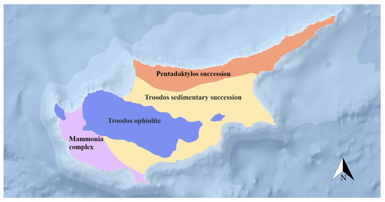
Figure 1.
Main geological zones of Cyprus.
2.2. Details among the Soil Properties
Reliable data are a major factor needed to perform a consistent factor analysis. Therefore, a very comprehensive literature survey was conducted to collect the required data with the desired soil properties. All the data have been gathered from the studies conducted on the soils of Cyprus included in governmental- and university-based research projects and peer- reviewed scientific articles.
Soil properties, including liquid and plastic limits, clay fraction, montmorillonite, and calcium carbonate content were recorded from 207 different soil samples carefully selected from the literature, assuring that the same methodologies were used to determine them. The original research that the soil properties derived from are the studies of Charalambous et al. [40], Hobbs et al. [41], Northmore et al. [42], Bilsel and Tuncer [43], Bilsel and Uygar [44], Nalbantoglu and Gucbilmez [45], Nalbantoglu and Tuncer [46], Bilsel [47,48], and Nalbantoglu [49].
All the soils are classified based on Unified Soil Classification System (USCS) for additional clarification. Based on this approach, three types of soils were noticed being used in this analysis. The dominant soil type is highly plastic clays (CH), representing 79% of the data, followed by low to medium plasticity clays (CL) and inorganic silts with high plasticity (MH) by a distribution of 12% and 9%, respectively.
The sampling method and the derived depth of the soils vary based on the original research. This includes disturbed and undisturbed sampling from surface excavations and rotary core drillings within various depths. Although contaminated soils were not particularly identified within the data, it might be a promising future topic [50,51].
The liquid limit of the soils ranges from 34% to 210%. This wide range of liquid limits indicates the different origins of soils with higher limits, which possibly belong to igneous-origin clays. Additionally, high values of liquid limits indicate the presence of the dominant montmorillonite mineral. The plastic limit varies between a wide range of 14% to 55%. The variety of the soil properties due to different geological origins and the fact that the soils were sampled all over Cyprus better represent the soils of the island. The basic descriptive properties of the selected soils, including range, mean, and standard deviation, are tabulated in Table 1. Also, further visualization of the data can be observed using the box and whiskers diagram in Figure 2.

Table 1.
Descriptive statistics of the soils.
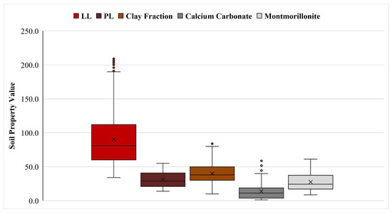
Figure 2.
Visual perspective of the soil properties.
3. Methodology
3.1. Research Framework
Geotechnical engineering was developed after a strong foundation under soils mechanics was formed. During this time, numerous ideas were developed and proven by scientists and engineers. This article is also based on principles of soil mechanics and applying these principles to geotechnics by using statistical science. The initial idea was triggered by finding a lack of research in geotechnical engineering related to factor analysis. In fact, there is little research in the geotechnical literature that utilized factor analysis as the main methodology. Combining the immense problematicity of clayey soils with multivariate analysis was a door-opening for new ideas. The idea was initially started by detecting an overlapping measure of the plasticity of clayey soils. These are the consistency limits, clay fraction and mineralogical effect. Based on this aspect, these measures can be combined into a single component that clearly defines the plasticity of soils. If such a model is formulated, then it can be used to assess the level of problematic significance of any soil, such as plasticity potential. However, this model would be only dedicated to plastic-characteristic of soils. Thus, any non-plastic soil cannot be used with this index.
The nature of every exploratory research requires a dedicated data set to begin with. Therefore, data gathering and selection have been performed meticulously. Special attention was paid to the validity and suitability of the data to determine a valid model. These were conducted by extensive checking of outliers among the data, adequacy of the data size, reliability, linearity, and normality of the data. If any irregularity was found, then variable transformations were performed to make the data set suitable for the analysis.
The variable transformation was followed by checking the applicability of the data set for factor analysis. These are extremely important tests before proceeding with the analysis. Any outcome might be misleading if the applicability of the factor analysis is ignored. The three main types of tests include the Kayser-Meyer-Olkin (KMO) test for sampling adequacy, Bartlett’s test of sample sphericity, and checking the intrinsic correlations among the data. If and only if these aforementioned tests have been checked, then the outcome of the factor analysis can be valid and applicable for future interpretations.
The next step of the research was to perform factor analysis. It is a deterministic way using a step-by-step procedure starting from factor extraction, determining communalities and component matrix, and calculating the factor scores. As a final step in this study, the gathered outcome from the analysis was interpreted to create a model defining the plasticity potential of soils. Every statistical step was performed using the statistical software package SPSS v26 (IBM Corp., Armonk, NY, USA). The overall research framework of the study is also given in Figure 3.
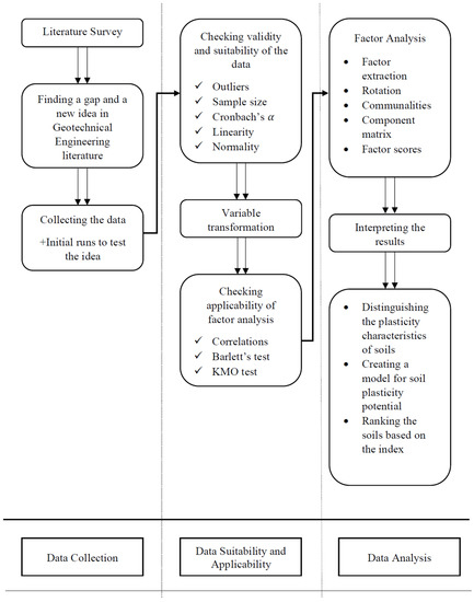
Figure 3.
The research flow chart.
3.2. A Concise Information on Factor Analysis
Factor analysis is a well-known multivariate statistical technique for data reduction. In its heart, it allows the determination of the overlapping measures of the common property among a variable set [52]. This measurement overlap is then clustered together into a single explaining variable, which is called a factor. Therefore, the initial stage of every factor analysis is to reduce multiple variables into a few explaining factors. In this study, these variables are the specifically chosen soil properties that define the soil plasticity characteristics. However, reducing the multiple variables into a few factors also reduces the amount of data explained. Therefore, it is crucial to have an explained variance as high as possible. Stevens [53] suggested the factors should explain the variability of at least 70% for a meaningful factor analysis.
If the factor analysis is a part of a subsequent analysis, such as in this study, then factor scores are generally used. The factor scores can be assigned to the individual soil property based on a weighted fashion. Consequently, these scores can be summed by various methods, weighted on an individual property or even used in regression analysis [54]. Considering this study is aimed at measuring plasticity potential, a higher potentially plastic soil would yield a higher factor score and vice versa. Eventually, the factor scores represent each soil and act as the new soil property value for future analysis.
Another fundamental aspect of factor analysis is its division into two distinguished parts. Exploratory factor analysis is the most used type that allows a researcher to reduce the number of variables by their common measures. The researcher might not be interested in the underlying relations between these variables. The confirmatory factor analysis requires a much more sophisticated research aspect. The researcher can perform an exploratory approach during the initial stage and then choose the variables purposefully to confirm the research hypothesis. In this study, both approaches were used accordingly.
The Principal Logic behind Factor Analysis
The main philosophy behind factor analysis is to derive an uncorrelated and linear combination of the original variables to explain the original variable as much as possible [55]. These linear combinations are the “factors”.
A factor analysis aims at partitioning the original variables into meaningful groups, which are the factors, so that each group explains a proportion of total variance within the data. This partitioning of factors is initiated by extracting the most explaining factor that accounts for the most variance. This is a progressive type of analysis until all the variance is explained by the extracted factors. Therefore, it is a crucial point to select the factors that have meaning in terms of the research and explains the data set as much as possible.
The first factor always explains the most variance in the data set and the last factor has the least explaining capability. The mathematical expression of these factors can be defined by the following equations (Equations (1) and (2)).
Here is the notation for each factor, is the loading of the variable within the given factor. can be taught as factor score coefficient or factor weights. represents the individual variables in the data set, is the mean of the variable and the is the specific factors. and are the subscripts that define the corresponding factor and variable, respectively. Considering the equations above, the weight within the factor is the most important coefficient in a research question. It allows labelling a factor based on research interest.
4. Initial Analyses and Findings
4.1. Validity and Suitability of Soil Properties
Almost every multivariate statistical analysis requires a data set that is specifically prepared before the analysis. The reliability of the data is almost always a certain measure. However, factor analysis is also sensitive to some other aspects of the data set. Extreme outliers within the data should be discarded. The overall sample size, meaning the soil count, should be adequate, a normal distribution is desired, and linearity should be achieved.
The first part of the suitability check of the soil properties is to distinguish the extreme outliers in the data set. The factor analysis is prone to fail if extreme outliers are included. Substantially lower or higher values within the data can affect the correlations and distort the factor analysis [56]. Since there is no singular way of measuring outliers, a few methods have been used to distinguish them. Histogram charts and scatter plots of each soil property have been checked since these charts can be used for visual interpretation. The box and whisker diagram is another valid way to spot extreme outliers. After careful examination, extreme outliers were especially found within the liquid limits and calcium carbonate contents. All outliers that may distort the analysis were discarded before proceeding to the next step.
The next option to validate the soil properties is a reliability analysis. Reliability is a measure of consistency among the data. For this purpose, a reliability coefficient namely Cronbach’s alpha can be used. In this study, Cronbach’s alpha was computed as 0.65 within liquid and plastic limits, clay content, calcium carbonate and montmorillonite content. A Cronbach’s alpha higher than 0.60 is regarded as sufficient in exploratory research [57,58]. Considering this outcome, the reliability of the soil properties is found to be valid and appropriate for this study.
The amount of data is another important consideration before initiating the analysis. However, there is no certain fact on the minimum amount [59]. Therefore, many studies have been made considering this topic, and many opinions have been yielded. According to Mertler and Reinhart [60], if there are several high-loading variables in the solution, such as above 0.80, then a data amount of 150 is sufficient (Appendix A). Guadagnoli and Velicez [61] and Stevens [53] noted that if there are four or more variables with factor loadings above 0.60, then any data size would be adequate. MacCallum et al. [62] suggested a minimum of 100 cases without any other consideration. Ho [63] and Hair et al. [58] have a much more unconservative approach, recommending a minimum sample size of five times the variable size and an optimum amount of ten times the variable size. All things considered, the sample size in this study can be marked as sufficient for the analysis.
Normal distribution among variables is generally an ignored aspect of factor analysis. Since the main aim of the factor analysis is to describe the relationship between variables, the normality does not affect the results drastically [64]. However, normal distribution among variables is recommended to enhance the solution. Therefore, the normal distribution of the five-soil property was checked individually. The highly regarded methods of checking the normality are using histogram charts, Q-Q pilots and a more direct measure based on skewness and kurtosis. After these checks, the normal distribution of the variables was detected to fail. Linearity of the data was also checked by scatter pilots and measuring the deviation from linearity. Whenever the normality and linearity of the soil properties failed, data transformation was carried out to enhance the analysis.
4.2. Applicability of the Analysis
After the soil properties have been validated and assessed as suitable, the next step is to check the factorability of the data set. The most common way to determine the applicability is by checking the intercorrelations among the variables and performing tests for sphericity and sampling adequacy.
Checking the correlations among the variables is a useful first step before proceeding to the analysis. This step is a basic examination of Pearson correlation coefficients between the variables. The relationship between the soil properties should be high enough so that there will be a meaningful interpretation of the underlying relations of soil properties. As a rule of thumb, Hahs-Vaughn [59] recommends searching for a coefficient of correlation of at least 0.30. Tabachnick and Fidell [64] and Hair et al. [58] approach this factorability check in a similar fashion. They suggested that there should be a substantial number of correlations above 0.30. In this study, the interrelations between the soil properties yielded coefficients of correlation above 0.30 (Table 2). Only calcium carbonate content is found to be negatively correlated with the rest of the soil properties. The reason behind this outcome is that liquid limit, plastic limit, clay content, and montmorillonite content tend to be positively correlated. Meaning that, if one of them increases the others should also increase and vice versa. However, this outcome also suggests that an increase in calcium carbonate content should decrease the rest of the soil properties. Considering, the liquid limit, plastic limit, clay content, and montmorillonite content increase the soil plasticity, the negative correlation of the calcium carbonate content is a sign of its negative effect on the plasticity characteristics of soils.
Table 2.
Pearson coefficients of correlation between the soil properties.
The factor analysis generates results based on the correlations between variables. If there is no correlation, then factor analysis cannot be performed. Bartlett’s test of sphericity measures the overall correlation among the variables and yields only one measurement [58]. If Bartlett’s test yields a significancy value below 0.05 then the analysis is statistically significant [63,65]. In this study, Bartlett’s test generated a significant value below 0.001. Therefore, the outcome of this study has statistical significance.
Another important consideration before performing the analysis is the measurement of the sampling adequacy. It is a measure of intercorrelations and factorability of the data set. The sampling adequacy, namely Kaiser-Meyer-Olkin (KMO) test, ranges from 0 to 1. If the KMO value is below 0.5, the factorability of the data set is rejected [66]. In this study, the KMO value is calculated as 0.807, which indicates the data are meritorious and factorable [66].
4.3. The Factor Analysis
4.3.1. Factor Extraction
Every factor analysis starts by extracting the desired or the required number of factors. Each of these factors represents a variable or a group of variables. There are some rules and extensions for determining the number of factors to be extracted. This extraction should be performed by determining the meaning and thus the labelling of the factor which is based on variable loadings within the factors. The extraction process can be followed by the rotation of the factors for a better interpretation of the analysis. Depending on the research objective, the calculation of the factor scores and assigning a score value on each variable is the final step. The decision progress for each phase is summarized in the following paragraphs.
The study includes five different soil properties that are acting as variables in the factor analysis (Table 3). The communality of the variables shows how much variance is explained by all factors. As stated by Ho [63], the minimum communality of each variable should be 0.2 to be retained in the analysis. In this study the minimum communality is calculated as 0.555 (Appendix A), therefore all the variables were retained.
Table 3.
The variables in this analysis and their corresponding notations.
The labelling of the factors depends on the loadings of the variables within a factor. Therefore, the method of interpretation is crucial before any misleading interpretation on the results. The factor matrix shows the loading of each soil property within the factor and can be interpreted as the correlation coefficients within the factor (Appendix A). However, it is an uninterpreted solution before any rotation is performed. Considering this aspect, the examination of the factor matrix reveals that the first factor heavily relies on consistency limits and montmorillonite content which is followed by the clay content. The calcium carbonate content has a negative sign with a relatively high loading of −0.593. This indicates that it has a negative relationship with the other soil properties when considering their effect as a whole. This concludes that the calcium carbonate content can be regarded as having a negative effect on soil plasticity characteristics. Investigation of the second factor shows that only calcium carbonate content has a high loading. This proves the fact that calcium carbonate content has a high impact on soil plasticity and should be included in the analysis. In this way, the negative effect of calcium carbonate contrary to the other properties is reflected in the analysis.
The examining and labelling of the factors were performed based on the purpose of the study and should be interpreted cautiously by the researchers. Based on the literature, there are three main rules to determine how many factors to extract. These include Kaiser’s rule of the eigenvalue [67], examining the scree plot and retaining the factors that explain at least 70% of the variance cumulatively. The Kaiser’s rule should be applied if the study includes 20 to 50 different variables [59] and is often found to misestimate the number of factors [68,69]. Therefore, it is not applicable in this study considering the variable size. The examination of the scree plot is very subjective, and the decision can change between different researchers [70]. Considering these uncertainties, the authors choose to extract the factors by examination of the factor loadings and the amount of variance explained. This type of approach is quite common in factor analysis if the researchers have a dedicated goal to prove and investigate [59,71].
Overall, two factors are extracted from the analysis. The first one includes the consistency limits, montmorillonite, and clay content. The second one represents the calcium carbonate content. The first factor explains 69.61% of the data and the second one explains 14.53%. This concludes that 84.14% of the total variance can be explained by considering only two factors which are reduced from five variables. Additionally, as mentioned before, the factors are divided and labelled into two that explain the soil plasticity characteristics both positively and negatively (Table 4).
Table 4.
The variables in this analysis and their corresponding contributions and remarks.
4.3.2. Factor Rotation
Factor rotation is a mathematical procedure that rotates the solution for a better interpretation of the results. The rotation does not change the factor extraction or the total variance explained. However, it is a geometrical interpretation feature that allows the observation of the effect of variables within a factor. This interpretation also changes the coefficients of variables and the distribution of variance; thus, factor scores are also affected. There are two types of rotations: orthogonal and oblique. Here, the main difference is that orthogonal rotation produces uncorrelated factors and oblique rotation vice versa [59]. The analyses indicated that the soil properties are correlated, and they all represent the plasticity characteristics of the soil regardless of the positive or negative effect. Therefore, altering one property will alter the overall plasticity. Consequently, the two extracted factors only include the variables to explain the plasticity-based characteristics due to confirmatory approach of the chosen factor analysis. Accordingly, the factors should be also correlated with each other. Based on these reasons, oblique rotation was chosen for the analysis. The rotated solution of the factors also clarified that the sole effect of calcium carbonate should be assigned as another factor (Appendix A). Also, if the soil properties are plotted based on their rotated loadings within the factor, distinguishable groups can be observed (Figure 4). These groups also indicate the validity of extracting two factors.
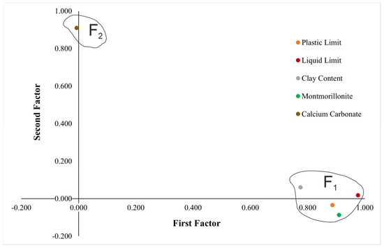
Figure 4.
Grouping of the extracted factors in rotated solution.
4.3.3. Factor Scores
After the extraction and rotation of the factors are carried out, factor scores can be calculated depending on the study. If the factor analysis is to be followed by a subsequent analytical procedure, then the use of factor scores essentially enhances the research. The factor scores are the estimated values of each variable within each factor if they are measured directly [64]. In other words, each factor score assigned to a variable represents the underlying theory of the study. Considering this study, the factor scores of the variables represent the plasticity potential of each soil. As a glimpse into the proceeding stage of this study, the higher the score means, the higher plasticity potential, thus, generally creating more problematic soil.
The theoretical perspective suggests that the calculation of the factor scores can be conducted in infinite ways [72]. Essentially, the factor scores are computed based on the factor loadings of each variable within the factor. Therefore, a high-loading variable will result in a higher score. As Gorsuch [72] suggested, there are many ways to calculate the factor score. These include the simple way of summing the factor loadings or taking the mean of these loadings to represent each variable. However, more sophisticated methods also exist: the regression approach, Bartlett method, and Anderson–Rubin approach. These methods tend to investigate the intercorrelations of the variables and factor loadings to yield a quantity called factor score coefficients. Among them, the main differences are related to the correlations of the factor scores. Such as the regression approach generates highest correlations between factors and factor scores. Bartlett’s method relates the factor scores considering only their own factor, and Anderson–Rubin produces uncorrelated scores.
In this study, the five-soil property was chosen for the investigation. These properties are essentially related and proved to be correlated as well. The produced factors must also be correlated based on the aim of the study. Considering the theoretical ways of producing the factor scores and the goal of the research, regression approach was chosen to assign a factor score for each soil. The corresponding factor score coefficients based on the regression approach is given in Appendix A.
5. Geotechnical Interpretations
5.1. Distinguishing the Plasticity Characteristics of Soils
The nature of the factor analysis assigns a factor score for each variable based on the number of factors. In this study, two factors have been extracted, therefore two distinctive factor scores were assigned to each soil. These factor scores are named as first and second-factor scores for simplicity.
These two factor scores measure the individual plasticity characteristics of each soil. The first score is the main controller of the soil plasticity since the total contribution to the analysis is 69.61% (Table 4) and represent the effect of consistency limits, clay fraction, and montmorillonite content. The second score directly correspond to the effect of the calcium carbonate on the plasticity of each soil with a contribution of 14.53%. In this study, the factor scores were interpreted in a way such that the plasticity of soil increases with an increase in factor score and vice versa.
An intriguing way to illustrate the factor scores can be achieved by using a two-dimensional cartesian coordinate system. If the first and second, factor scores are plotted in x- and y-axes, a data scatter of the scores’ can be achieved. This kind of scatter can be easily gathered by using any statistical software. However, the interpretation of such plots can be sophisticated and generally requires a dedicated research perspective.
The first and second factor scores can be seen as a scatter plot in Figure 5. The vertical- and horizontal-axes represent the first and second factor scores, respectively. An added simplification is performed by assigning colours to each soil based on USCS. This colourizing of soil groups vastly clarified the data scatter. A first look into the figure indicates a grouping of soils to some degree. However, this grouping is only valid for CL and MH types of soils. This confirms a valuable conclusion for CL and MH soils that they have a discrete character in terms of soil plasticity. In consequence, one should expect a rather different plastic behaviour under certain circumstances.
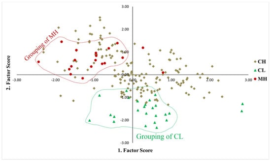
Figure 5.
Grouping of different soil types indicate the plasticity characteristics.
Low plasticity clayey soils (CL) are all on the negative side of the first factor score. Since the first factor score contributed the most to the soil problematicity, it is clearly observable that CL soils are generally less problematic than the CH and MH soils. However, this is a generalized outcome, and it is clearly visible that some CH soils also have the same problematicity as CL soils.
Contrarily, almost all the medium–high plasticity silty clayey soils (MH) are on the positive side of the first factor score and the negative side on the second factor score. This indicates that the plasticity-based characteristics of MH soils are distinctively different and yield more problems than CL soils. Also, it is clearly visible that the calcium carbonate, i.e., second factor score, has a profound control on the plastic behaviour of MH soils.
On the other hand, the CH soils have almost equal distribution along the scatter plot. This concludes that there is no significant soil property that controls the plastic behaviour of CH soils. Therefore, the plasticity of CH soils is rather controlled equally in a balanced way by consistency limits, clay fraction, and mineralogy.
5.2. Measuring the Unified Plasticity Potential of Soils
In the previous sections, factor analysis was performed on the data for various purposes. One of the first aims was to reduce the soil properties from five to two and finding the hidden interrelations between them, such as uncovering the negative effect of calcium carbonate on soil plasticity. Lastly, two different factor scores were assigned to each soil based on the regression approach. These factor scores were then analysed to distinguish the plasticity characteristics, and possibly the behaviour, of CL, CH, and MH soils.
The next part of this study is to create an empirical approach to quantitively measure the plasticity characteristics of clayey soils. Considering each factor score is a measurement of the soil plasticity, they can be used in a way to accomplish this purpose. One of the most convenient ways is to simply sum the first and second scores to have a final value that represents each soil. Considering each factor score has a different contribution to soil plasticity, this kind of direct approach would not be representative. In this study, the contribution of each factor score has been taken into account and a final resultant factor score was calculated by using a weighted summation approach. Creating a resultant factor score is the initial step to measure the plasticity potential of each soil. The equation below shows the calculation of the resultant value (Equation (3)).
Here, is the resultant factor score, represents the first factor score and is the second factor score. Although the above expression yields a weighted score for each soil, it is still a non-standardized way to represent each soil. Also, the value of can vary between negative and positive numbers, which is eventually difficult to interpret. Therefore, a standardized approach was chosen in this study. The standardization of the resultant factor score should be conducted in a range that any soil assigned with a value can be easily distinguished. Therefore, the is standardized between 0 and 100 by considering the minimum and maximum values of the resultant factor score assigned to the soils (Equation (4)).
Here, the standardized is the plasticity potential of soils. This expression assigns a particular value between 0 and 100 to each soil. As this value increases, soil plasticity also increases. Therefore, the soil with the least plasticity potential should yield zero, and the soil that shows the most plasticity should be assigned 100.
The validation of this model is critical for the purpose of this research. Considering the plasticity index is a direct approach for measuring plasticity and is widely accepted in practice, this model should coincide if the soils are ranked based on only using the PI. Meaning that if the PI increases, the plasticity potential should also increase in a parallel way. However, the theory of this study is clear; the PI measures the plasticity but does not incorporate the effect of other soil properties. That is the reason that other soil properties related to PI, but not PI itself, were included in the analysis and eventually reduced to a standardized definition of soil plasticity. These facts should be clearly observed in order to validate the theory. Therefore, all the soils were ranked based on the plasticity potential from top-to-bottom and bottom-to-top order. This study’s ranking is then compared to the PI ranking for validation. Table 5 and Table 6 represent the most and the least plastic soils based on these rankings, respectively. Also, each row indicates individual soils and shows the consistency limits, clay fraction, calcium carbonate, and montmorillonite content.
Table 5.
The ranking of the top 10 soils that shows the most plasticity.
Table 6.
The ranking of the bottom 10 soils that shows the least plasticity.
An inspection of Table 5 and Table 6 directly reveals that there is a strong parallel relation between the PI-based ranking and this study’s ranking. Considering the top 10 soils, there is a very slight difference in ranking on most of the soils, only the sixth and eighth soils show a reasonable difference. The reason for this disparity is related to the considerably lower plasticity index of the sixth and eighth soils. However, careful examination of the factor analysis shows that the standardized score, i.e., plasticity potential, was calculated by assuming the consistency limits, clay fraction and montmorillonite content contribute to the plasticity of soils almost equally. This conclusion can be seen by examining the factor score coefficients in Appendix A. Examination of the least potentially plastic soils (Table 6) also coincides with the finding of the most potentially plastic soils. Therefore, this model can be assumed to work in a wide range of soil plasticity.
The above-mentioned facts justify that a quantitative model can be formulated to measure the plasticity potential of soils. Presently, the finding is very definite: the standardized score is the plasticity potential of soils that can be assigned from 0 to 100. If this model is formulated, then one could assess the plasticity potential of any soil easily. However, there should be a reliable way to predict this plasticity potential. For this purpose, some soil parameters that are easy to derive that represent different properties of the soil should be used. Considering the liquid and plastic limits, clay fraction, montmorillonite and calcium carbonate content were already used in the analysis. Therefore, if these soil properties are used for the prediction, then there will be an overlapping measure within the model. Which invalidates the whole theory. However, the plasticity index itself was not an input parameter in the analysis, therefore the PI is one of the soil properties that can be used in a way to predict the soil plasticity potential.
Figure 6 shows the relationship between this model and PI. The relationship between this model and PI yielded a very strong correlation coefficient of 0.908. This indicates the PI can be confidently used to predict the unified plasticity potential of the soils. The elemental aspect of using this model instead of PI alone is that in this study the plasticity potential of soils was measured by five different soil properties. However, the PI alone is rather a sole parameter. Therefore, using the PI to predict this study’s plasticity model allows the user to evaluate the soil plasticity in a more refined and realistic way. Therefore, using this model should represent a much more accurate way of soil plasticity. In fact, one can assume that this model is a modified plasticity index to some degree. Also, the plasticity potential is formulated as a logarithmic function of the plasticity index as shown in the equation below.
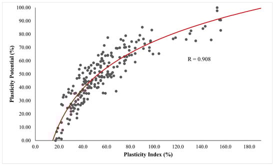
Figure 6.
The relationship between plasticity potential and plasticity index as a logarithmic function.
The other soil property that can be used to assess the plasticity potential is the sand content. However, sand particles themselves do not contribute to soil plasticity; therefore, sand content was not included in the factor analysis. Nevertheless, an increase in sand content should reduce the plasticity of soil in general. The reason for that is highly connected to the ratio of cohesive and noncohesive materials in the soil. Thus, a decrease in sand content tends to increase the fine content which can contribute to soil plasticity. This fact is proven by demonstrating the relationship between the plasticity potential model in Figure 7. It is clearly observable that a decrease in sand content increases the plasticity of the soil. The most reasonable way of expressing this relation was found as a linear function yielding a coefficient of correlation of 0.704. The direct relationship between the PI and sand content was also measured which generated a coefficient of 0.519 for the same function type. This noticeable difference indicates the relationship between sand content and plasticity potential is increased by 36%. This outcome demonstrates that unifying the soil properties into one explaining model improves and even uncovers the theoretical relationships. In this circumstance, the linear function was found representative of the relation between plasticity potential and sand content (Equation (6)). The sand content is expressed as SC in the equation for clarity.
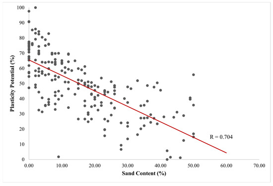
Figure 7.
The relationship between sand content and plasticity potential as a linear function.
Since two different soil properties can be used to assess the plasticity potential, two of them should be combined into a singular expression that defines this model. This can be carried out by using regression analyses. However, regression analysis has many varieties such as using single or multiple variables in a linear function to predict the unknown quantity or a more complex version that uses nonlinear relations with many variables. The regression analysis is not the main subject of this study but rather a statistical tool therefore it will not be explained in detail. A classic nonlinear expression is given in Equation (6) for representation purposes. Where, x and z are the variables, a and b are the parameter estimates, and c is the constant of the equation. This formula is a typical representation of a nonlinear relationship which includes more than one function type.
All things considered, nonlinear regression is one of the most complex regression types that require the user to decide the types of functions and the presence of constants. In this study, the relationship of PI and sand content with plasticity potential is both nonlinear and linear, therefore it is logical to adopt an overall nonlinear function for best-fitting purposes. Considering, the relationship of PI and sand content with plasticity potential was individually defined by logarithmic and linear functions, respectively. The nonlinear regression model should also be assigned in that way. Also, the parameter’s estimate and a constant were included in the regression. Therefore, the below expression was run to predict the best-suited equation of plasticity potential (Equation (8)).
Here, y is the plasticity potential, x is the plasticity index, z is the sand content, a and b are the parameter’s estimates, and c is the constant of the function. Considering the above equation, the nonlinear regression model was tested and found to be best suited as the following expression (Equation (9)). This relationship of PI and sand content to plasticity potential yielded a very high coefficient of correlation of 0.944. This high value of the coefficient proves that Equation (9) has an undeniable statistical significancy to represent the plasticity potential of soils in a unified form.
Considering Equation (9), which includes two different soil properties, Equations (5) and (6) should not be used to determine the exact value of the plasticity potential. Rather, the interested user should only utilize Equation (9) to define the unified plasticity potential of soils. Equation (9) works with a minimum plasticity index of 9%, thus the user should assign the plasticity potential as zero for lesser values of PI. In this sense, if any outcome is negative or greater than 100, then the plasticity potential should be assigned as 0 and 100, respectively.
Also, the authors proposed to the interested user to use the following figures for quick assessment. In this case, Figure 8 is best suited for greater values of the plasticity index and Figure 9 for lesser values. Additionally, the extent of this study includes sand content between 0 and 50 percent. Therefore, Figure 8 and Figure 9 have been created by extrapolating the sand content up to 80%. The 60 and 80% lines are theoretical and should be used cautiously. Especially, where sand content exceeds 50% with very high plasticity index, above 150%, this model should be a rough guidance concerning the soil plasticity potential rather than assigning a definitive value.
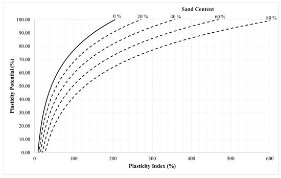
Figure 8.
Visual representation of plasticity potential best suited for greater plasticity index values.
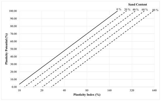
Figure 9.
The plasticity potential of soils that are best suited for lesser plasticity index values.
The factor analysis was carried out after transforming the soil properties to normal distribution. Based on this fact, the plasticity potential between 0 and 100 was also assigned to the soils as normally distributed. This distribution can be used to categorize the plasticity potential statistically. For this purpose, the three-sigma rule also as known as the 68-95-99.7 rule was applied to the data [73]. This rule allows the researcher to categorize the data in percentages based on certain intervals, if the data are normally distributed. These certain percentages are 2.35, 15.85, 49.85, 83.85, and 97.85 and correspond to the plasticity potential of 5.4, 27.5, 48.7, 70.0, and 85.6, respectively. To avoid any confusion, the percent of 15.85 corresponds to a plasticity potential from 0 to 27.5.
Based on this approach, the plasticity potential is divided into six categories starting from negligible to severe plasticity, as shown in Table 7. A generalized indication of these categories is also represented in terms of effective angle of internal friction , undrained shear strength (, compressibility while compacted and saturated and volume change potential upon wetting and drying. These positive and negative relationships of plasticity potential between material properties are a generalized derivation from the literature [74,75,76,77,78,79]. Considering there is a positive logarithmic relation between PI and plasticity potential, a drastic increase in PI should also increase the plasticity potential. The exact relations can be formulized by extensive laboratory work, which is out of the scope of this study. Although this model allows the user to easily access the desired range of plasticity potential, he/she should be aware of the appropriate material selection based on the project or research needs.
Table 7.
Assessment of plasticity potential and corresponding remarks.
5.3. Recommended Applications of the Unified Plasticity Potential Model
The development of the plasticity potential of soils as a unified approach allows the interested user to determine the plasticity potential of the soil with only two easily derived soil properties. Authors highly recommend using this model on large-scale projects as in the following guidance. Localized micro zonation maps can be produced by systematically collecting as many soil samples as possible and then simply deriving PI and sand content only to assign a plasticity potential value to each of them. Then, these values should be integrated with geographical coordinates of each sample on a Geographical Information Systems based solution. Consequently, desired maps can be derived indicating the six degrees of plasticity potential colorized as individual contours. These maps can be used to quickly assess the plasticity potential of the soil within the location of interest. However, this kind of work requires a systematic study dedicated to this purpose and depending on the scale of the project it might last from a few months to several years.
Another useful aspect of this model can be found in the assessment of the liquefaction potential of fine-grained soils. The liquefaction phenomenon is generally observed on mainly coarse-grained soils especially on clean sands in loose state [80]. A ground-shaking motion such as seismic activity vibrates the saturated soil particles which causes a sudden loss of strength under the structures. Eventually, the structure acts as its foundation laid upon a liquid-like material that causes the structure to tilt over or sink into the soil. Considering the liquefaction of soils causes settlement and bearing capacity problems, the detection of a possible liquefiable soil is critical. Although coarse-grained soils are more prone to this type of behaviour, even fine-grained soils can also liquefy. Wang [81], Polito [82], Seed et al. [83], Bray et al. [84], Bray and Sancio [85] are notable researchers concerning the liquefaction of fine-grained soils. All of them evaluated the plasticity index of soil as the main triggering parameter. The unified plasticity potential of soils is assessed by using the plasticity index as well as the sand content which is another major parameter for soil liquefaction. Therefore, the authors recommend gathering the liquefied fine-grained soils from the site and performing a series of laboratory work to determine the plasticity index and the sand content. This can also be achieved by a literature review of the liquefied clayey soils. The next step would be to distinguish the range of the plasticity potential of the soils that liquefied. By doing so, interested practising academics or engineers should easily determine the severity of the soil based on liquefaction potential.
This model can also be integrated into tender documents especially in earth work projects. This should be performed by a knowledgeable scientist or an engineer. This person should determine the maximum allowable limit or range for plasticity potential depending on the project’s needs. By doing so, the contractor will be able to easily gather the required soil material from a near borrow location after preliminary laboratory tests.
6. Conclusions
The use of factor analysis revealed that consistency limits, clay content, montmorillonite, and calcium carbonate content influence the plasticity characteristics of soils. These soil properties were reduced into two distinctive hypothetical variables to better interpolate the plasticity of soils. The analysis also revealed that clay content, consistency limits and montmorillonite content are all at once overlapping measures of plastic behaviour.
After refining the plasticity of soils by factor analysis, the relation with sand content is improved. A regression analysis has been made to prove this fact. It is observed that there is a notable improvement in the coefficient of correlation. This concludes that the use of the proposed model would ideally yield a more accurate relationship between soil properties. This in fact, also indicates the use of the model and better represents the true plasticity characteristics of soils.
Furthermore, discovering these relations indicates that this model better represents the plasticity of soils than using only laboratory-derived plasticity index. Therefore, considering the wide usage of the plasticity index in practical applications, as an input parameter, needs refinement.
It is proven that the direct laboratory measures of plasticity do not completely incorporate the effect of other correlated soil properties. Therefore, the analysis also yielded the fact that characterising and classifying soils based on their plastic characteristics would be more accurate using this model rather than the plasticity index.
All 207 soils were assigned individual factor scores each representing the plasticity characteristics. These soils were ranked based on the plasticity index and factor scores. A distinct observation was noticed that some of the soils were reordered when ranked by factor scores. These changes in the sorting are mainly due to the calculation procedure of the plasticity potential of soils, where each soil property, except calcium carbonate, was determined to best fit with an approximately equal contribution to soil plasticity.
It is demonstrated that the plasticity characteristics of CL and MH soils are noticeably different. The plasticity of MH soils is controlled by calcium carbonate content. Some CL and CH soils were found to have similar plasticity characteristics. On the other hand, the plasticity of CH soils is controlled by consistency limits, clay content, and mineralogy altogether. There is no clear indication that one of the soil properties is more dominant than any other on the plasticity of CH soils. This contributes as a major finding for CH soils.
The exploratory nature of the factor analysis also indicated that the natural calcium carbonate content affects the plasticity characteristics of the soils negatively. This outcome is directly observable by examining the soil properties loadings within the first factor, and it is partially hidden before performing this analysis. This outcome is also supported by the negative interrelation of the calcium carbonate content with the rest of the soil properties. Considering the positive effect of the liquid limit, plastic limit, clay, and montmorillonite content on the plasticity, the contrary relation of calcium carbonate indicated the negative effect on soil plasticity.
Many statistical analyses require a trial-and-error procedure during the initial stages. In this case, the authors found out that the factor rotation changes the induvial factor scores. Thus, the overall representation of plasticity characteristics, as well as the proposed risk model along with the ranking of soils, change. Therefore, the authors recommend choosing the most appropriate method of factor rotation based on the aim of the study to prevent any misleading conclusion.
The lack of statistics-related geotechnical research in Cyprus is the main reason that triggered this study. Therefore, only the available and reliable geotechnical data were collected. Eventually, this aspect yielded only CL, CH and MH types of soils. Acknowledging this, the authors recommend using this model with C and M groups of soils. However, this research is based on very strong statistical fundamentals. Hence, the authors believe that any type of similar research would not change the elemental findings of this study but rather enhance it for broader applications.
Author Contributions
Conceptualization, B.S.F. and H.B.; methodology, B.S.F.; validation, B.S.F. and H.B.; investigation, B.S.F.; data curation, B.S.F.; writing—original draft preparation, B.S.F.; writing—review and editing, H.B.; visualization, B.S.F.; supervision, H.B. All authors have read and agreed to the published version of the manuscript.
Funding
This research received no external funding.
Institutional Review Board Statement
Not applicable.
Informed Consent Statement
Not applicable.
Data Availability Statement
Contact the corresponding author for academic use.
Acknowledgments
The author (B.S.F.) thanks Abdullah Ekinci from Middle East Technical University and Eris Uygar from Eastern Mediterranean University for their contributions from the initial to the final stage of the study.
Conflicts of Interest
The authors declare no conflict of interest.
Appendix A. Supplementary Tables Related to the Factor Analysis
Table A1.
The variables’ original loadings within the factors.
Table A1.
The variables’ original loadings within the factors.
| LL | PL | Clay Content | Montmorillonite | ||
|---|---|---|---|---|---|
| F1 | 0.951 | 0.894 | 0.726 | 0.947 | −0.593 |
| F2 | 0.177 | 0.125 | 0.168 | 0.079 | 0.803 |
Table A2.
The variables’ loadings after oblique rotation.
Table A2.
The variables’ loadings after oblique rotation.
| LL | PL | Clay Content | Montmorillonite | ||
|---|---|---|---|---|---|
| F1 | 0.977 | 0.891 | 0.767 | 0.909 | −0.006 |
| F2 | 0.021 | −0.026 | 0.053 | −0.086 | 0.996 |
Table A3.
The communalities of the soil properties.
Table A3.
The communalities of the soil properties.
| LL | PL | Clay Content | Montmorillonite | ||
|---|---|---|---|---|---|
| Extracted value | 0.937 | 0.815 | 0.555 | 0.904 | 0.997 |
Table A4.
Coefficients of the factor scores for each soil property.
Table A4.
Coefficients of the factor scores for each soil property.
| LL | PL | Clay Content | Montmorillonite | ||
|---|---|---|---|---|---|
| F1 | 0.309 | 0.282 | 0.243 | 0.286 | 0.012 |
| F2 | 0.036 | −0.013 | 0.064 | −0.073 | 0.994 |
References
- Wesley, L.D. Residual Strength of Clays and Correlations Using Atterberg Limits. Geotechnique 2003, 53, 669–672. [Google Scholar] [CrossRef]
- Kayabali, K.; Tufenkci, O.O. Shear Strength of Remolded Soils at Consistency Limits. Can. Geotech. J. 2010, 47, 259–266. [Google Scholar] [CrossRef]
- O’Kelly, B.C. Atterberg Limits and Remolded Shear Strength? Water Content Relationships. Geotech. Test. J. 2013, 36, 939–947. [Google Scholar] [CrossRef]
- Karakan, E.; Demir, S. Relationship between Undrained Shear Strength with Atterberg Limits of Kaolinite/Bentonite–Quartz Mixtures. Int. J. Eng. Res. Dev. 2018, 10, 92–102. [Google Scholar] [CrossRef]
- Mawlood, Y.; Mohammed, A.; Hummadi, R.; Hasan, A.; Ibrahim, H. Modeling and Statistical Evaluations of Unconfined Compressive Strength and Compression Index of the Clay Soils at Various Ranges of Liquid Limit. J. Test. Eval. 2021, 50. [Google Scholar] [CrossRef]
- Giasi, C.I.; Cherubini, C.; Paccapelo, F. Evaluation of Compression Index of Remoulded Clays by Means of Atterberg Limits. Bull. Eng. Geol. Environ. 2003, 62, 333–340. [Google Scholar] [CrossRef]
- Mandhour, E.A. Prediction of Compression Index of the Soil of Al-Nasiriya City Using Simple Linear Regression Model. Geotech. Geol. Eng. 2020, 38, 4969–4980. [Google Scholar] [CrossRef]
- Spagnoli, G.; Shimobe, S. Statistical Analysis of Some Correlations between Compression Index and Atterberg Limits. Environ. Earth Sci. 2020, 79, 532. [Google Scholar] [CrossRef]
- Gurtug, Y.; Sridharan, A. Prediction of Compaction Characteristics of Fine-Grained Soils. Geotechnique 2002, 52, 761–763. [Google Scholar] [CrossRef]
- Di Matteo, L.; Bigotti, F.; Ricco, R. Best-Fit Models to Estimate Modified Proctor Properties of Compacted Soil. J. Geotech. Geoenviron. Eng. 2009, 135, 992–996. [Google Scholar] [CrossRef]
- Đoković, K.; Rakić, D.; Ljubojev, M. Estimation of Soil Compaction Parameters Based on the Atterberg Limits. Min. Metall. Eng. Bor 2013, 1–16. [Google Scholar] [CrossRef]
- Idris, A.; Waziri, M.I.; Abdulfatah, A.Y.; Umar, M. Modelling and Prediction of Compaction Parameters Based on Atterberg Limits and Clay Content. J. Eng. Tech. 2014, 9, 24–27. [Google Scholar]
- Prasanna, H.S.; Harshitha, D.; Singh, D.K.; Krishnegowda, K.H.; Suhruth, S. Correlation of Compaction Characteristics of Fine-Grained Soils Using Atterberg Limits. Int. J. Eng. Res. Technol. 2017, 6. [Google Scholar] [CrossRef]
- Saikia, A.; Baruah, D.; Das, K.; Rabha, H.J.; Dutta, A.; Saharia, A. Predicting Compaction Characteristics of Fine-Grained Soils in Terms of Atterberg Limits. Int. J. Geosynth. Ground Eng. 2017, 3, 1–9. [Google Scholar] [CrossRef]
- Firomsa, W.; Emer Tucay Quezon, P. Parametric Modelling on the Relationships between Atterberg Limits and Compaction Characteristics of Fine-Grained Soils. Int. J. Adv. Res. Eng. Appl. Sci. 2019, 8, 1–20. [Google Scholar]
- Hussain, A.; Atalar, C. Estimation of Compaction Characteristics of Soils Using Atterberg Limits. IOP Conf. Ser. Mater. Sci. Eng. 2020, 800, 012024. [Google Scholar] [CrossRef]
- Ahmed, S.M.; Agaiby, S.S. Strength and Stiffness Characterization of Clays Using Atterberg Limits. Transp. Geotech. 2020, 25, 100420. [Google Scholar] [CrossRef]
- Fener, M.; Kahraman, S.; Bay, Y.; Gunaydin, O. Correlations between P-Wave Velocity and Atterberg Limits of Cohesive Soils. Can. Geotech. J. 2005, 42, 673–677. [Google Scholar] [CrossRef]
- Earl, D. To Determine If There Is a Correlation between the Shrink Swell Index and Atterberg Limits for Soils within the Shepparton Formation. Ph.D. Thesis, University of Southern Queensland, Toowoomba, Australia, 2005. [Google Scholar]
- Yukselen, Y.; Kaya, A. Prediction of Cation Exchange Capacity from Soil Index Properties. Clay Min. 2006, 41, 827–837. [Google Scholar] [CrossRef]
- Dolinar, B. Predicting the Hydraulic Conductivity of Saturated Clays Using Plasticity-Value Correlations. Appl. Clay Sci. 2009, 45, 90–94. [Google Scholar] [CrossRef]
- Ercanoglu, M.; Gokceoglu, C. Assessment of Landslide Susceptibility for a Landslide-Prone Area (North of Yenice, NW Turkey) by Fuzzy Approach. Environ. Geol. 2002, 41, 720–730. [Google Scholar] [CrossRef]
- Ercanoglu, M.; Gokceoglu, C.; Van Asch, T.W.J. Landslide Susceptibility Zoning North of Yenice (NW Turkey) by Multivariate Statistical Techniques. Nat. Hazards 2004, 32, 1–23. [Google Scholar] [CrossRef]
- Pensomboon, G. Landslide Risk Management and Ohio Database a Dissertation. Ph.D. Thesis, University of Akron, Akron, OH, USA, 2007. [Google Scholar]
- Halvithana, M.S.; Jayathissa Aus Alawwa, A.G.; Lanka, S. Combined Statistical and Dynamic Modeling for Real Time Forecasting of Rain Induced Landslides in Matara District, Sri Lanka-a Case Study. Master’s Thesis, Eberhard Karls University of Tübingen, Tübingen, Germany, 2010. [Google Scholar]
- Quintela, A.; Costa, C.; Terroso, D.; Rocha, F. Liquid Limit Determination of Clayey Material by Casagrande Method, Fall Cone Test and EBS Parameter. Mater. Technol. 2014, 29, B82–B87. [Google Scholar] [CrossRef]
- Moghadami, M.; Mortazavi, A. Development of a Risk-Based Methodology for Rock Slope Analysis. Int. J. Civ. Eng. 2018, 16, 1317–1328. [Google Scholar] [CrossRef]
- Santos, A.E.M.; Lana, M.S.; Pereira, T.M. Rock Mass Classification by Multivariate Statistical Techniques and Artificial Intelligence. Geotech. Geol. Eng. 2021, 39, 2409–2430. [Google Scholar] [CrossRef]
- Moosavi, S.A.; Mohammadi, M. Development of a New Empirical Model and Adaptive Neuro-Fuzzy Inference Systems in Predicting Unconfined Compressive Strength of Weathered Granite Grade III. Bull. Eng. Geol. Environ. 2021, 80, 2399–2413. [Google Scholar] [CrossRef]
- Mahdizadeh, M.; Afzal, P.; Eftekhari, M.; Ahangari, K. Geomechanical Zonation Using Multivariate Fractal Modeling in Chadormalu Iron Mine, Central Iran. Bull. Eng. Geol. Environ. 2022, 81, 1–29. [Google Scholar] [CrossRef]
- Szabó, N. Dry Density Derived by Factor Analysis of Engineering Geophysical Sounding Measurements. Acta Geod. Geophys. Hung. 2012, 47, 161–171. [Google Scholar] [CrossRef]
- Szabó, N.P.; Dobróka, M.; Drahos, D. Factor Analysis of Engineering Geophysical Sounding Data for Water-Saturation Estimation in Shallow Formations. Geophysics 2012, 77, WA35–WA44. [Google Scholar] [CrossRef]
- Balogh, G.P. New Statistical Approach for Water Content Determination in Shallow Geological Environment. In Proceedings of the MultiScience-XXX. microCAD International Multidisciplinary Scientific Conference, Miskolc, Hungary, 21–22 April 2016. [Google Scholar]
- Kariuki, P.C.; van der Meer, F. Issues of Effectiveness in Empirical Methods for Describing Swelling Soils. Int. J. Appl. Earth Obs. Geoinf. 2003, 4, 231–241. [Google Scholar] [CrossRef]
- Gorsevski, P.V.; Gessler, P.; Foltz, R.B. Spatial Prediction of Landslide Hazard Using Logistic Regression and GIS. In Proceedings of the 4th International Conference on Integrating GIS and Environmental Modeling (GIS/EM4), Banff, AB, Canada, 2–8 September 2000. [Google Scholar]
- Kariuki, P.C.; Van der Meer, F.D. Swelling Clay Mapping for Characterizing Expansive Soils; Results from Laboratory Spectroscopy and Hysens Dais Analysis. In Proceedings of the 3rd EARSeL Workshop on Imaging Spectroscopy, Oberpfaffenhofen, Germany, 13–16 May 2003. [Google Scholar]
- Masoud, A.A. Geotechnical Evaluation of the Alluvial Soils for Urban Land Management Zonation in Gharbiya Governorate, Egypt. J. Afr. Earth Sci. 2015, 101, 360–374. [Google Scholar] [CrossRef]
- Liang, Z.; Wang, C.; Han, S.; Ullah Jan Khan, K.; Liu, Y. Classification and Susceptibility Assessment of Debris Flow Based on a Semi-Quantitative Method Combination of the Fuzzy C-Means Algorithm, Factor Analysis and Efficacy Coefficient. Nat. Hazards Earth Syst. Sci. 2020, 20, 1287–1304. [Google Scholar] [CrossRef]
- Liang, Z.; Wang, C.; Duan, Z.; Liu, H.; Liu, X.; Khan, K.U.J. A Hybrid Model Consisting of Supervised and Unsupervised Learning for Landslide Susceptibility Mapping. Remote. Sens. 2021, 13, 1464. [Google Scholar] [CrossRef]
- Charalambous, M.; Hobbs, P.R.N.; Northmore, K.J. Supplementary Geotechnical and Mineralogical Data for Cohesive Soil Samples from Selected Sites across Cyprus; British Geological Survey: Nottingham, UK, 1986. [Google Scholar]
- Hobbs, P.R.N.; Loukaides, G.; Petrides, G. Geotechnical Properties and Behaviour of Pliocene Marl in Nicosia, Cyprus; British Geological Survey (B.G.S) & Geological Survey Department of Cyprus (G.S.D): Nottingham, UK, 1986; 288p. [Google Scholar]
- Northmore, K.J.; Charalambous, M.; Hobbs, P.R.N.; Petrides, G. Engineering Geology of the Kannaviou, ‘Melange’ and Mamonia Complex Formations: Phiti/Statos Area, SW Cyprus; Engineering Geology of Cohesive Soils Associated with Ophiolites, with Particular Reference to Cyprus; British Geological Survey (B.G.S): Nottingham, UK, 1986. [Google Scholar]
- Bilsel, H.; Tuncer, E.R.; Gazimagusa, N.C. Cyclic Swell-Shrink of Structured Soils in a Semi-Arid Climate. In Proceedings of the 52nd Conference of the Canadian Geotechnical Society, Regina, SK, Canada, 24–27 October 1999; pp. 25–27. [Google Scholar]
- Bilsel, H.; Uygar, E.; Gazimagusa, N.C. The Effect of Repeated Wetting-Drying on the Hydraulic Properties of Konnos Clay. In Proceedings of the 53rd Canadian Geotechnical Conference, Montreal, QC, Canada, 15–18 October 2000. [Google Scholar]
- Nalbantoglu, Z.; Gucbilmez, E. Improvement of Calcareous Expansive Soils in Semi-Arid Environments. J. Arid. Environ. 2001, 47, 453–463. [Google Scholar] [CrossRef]
- Nalbantoglu, Z.; Tuncer, E.R. Compressibility and Hydraulic Conductivity of a Chemically Treated Expansive Clay. Can. Geotech. J. 2001, 38, 154–160. [Google Scholar] [CrossRef]
- Bilsel, H. Hydraulic Properties of Compacted Calcareous and Saline Soils of Cyprus. In Proceedings of the XIIIth European Conference on Soil Mechanics and Geotechnical Engineering, Prague, Czech Republic, 25–28 August 2003; pp. 1–46. [Google Scholar]
- Bilsel, H. Hydraulic Properties of Soils Derived from Marine Sediments of Cyprus. J. Arid. Environ. 2004, 56, 27–41. [Google Scholar] [CrossRef]
- Nalbantoğlu, Z. Effectiveness of Class C Fly Ash as an Expansive Soil Stabilizer. Constr. Build. Mater. 2004, 18, 377–381. [Google Scholar] [CrossRef]
- Qu, J.; Li, Z.; Wu, Z.; Bi, F.; Wei, S.; Dong, M.; Hu, Q.; Wang, Y.; Yu, H.; Zhang, Y. Cyclodextrin-Functionalized Magnetic Alginate Microspheres for Synchronous Removal of Lead and Bisphenol a from Contaminated Soil. Chem. Eng. J. 2023, 461, 142079. [Google Scholar] [CrossRef]
- Qu, J.; Yuan, Y.; Zhang, X.; Wang, L.; Tao, Y.; Jiang, Z.; Yu, H.; Dong, M.; Zhang, Y. Stabilization of Lead and Cadmium in Soil by Sulfur-Iron Functionalized Biochar: Performance, Mechanisms and Microbial Community Evolution. J. Hazard. Mater. 2022, 425, 127876. [Google Scholar] [CrossRef]
- Williams, F.; Monge, P. Reasoning with Statistics how to Read Quantitative Research; Harcourt College Publishers: London, UK, 2001; ISBN 0155068156. [Google Scholar]
- Stevens, J.P. Applied Multivariate Statistics for the Social Sciences; Routledge: New York, NY, USA, 2012; ISBN 1136910697. [Google Scholar]
- DiStefano, C.; Zhu, M.; Mindrila, D. Understanding and Using Factor Scores: Considerations for the Applied Researcher. Pract. Assess. Res. Eval. 2009, 14, 20. [Google Scholar]
- Johnson, R.A.; Wichern, D.W. Applied Multivariate Statistical Analysis; Prentice Hall: Hoboken, NJ, USA, 2002. [Google Scholar]
- Krishnan, V. Constructing an Area-Based Socioeconomic Index: A Principal Components Analysis Approach; Early Child Development Mapping Project: Edmonton, AB, Canand, 2010. [Google Scholar]
- Robinson, J.P.; Shaver, P.R.; Wrightsman, L.S. Criteria for Scale Selection and Evaluation. Meas. Personal. Soc. Psychol. Attitudes 1991, 1, 1–16. [Google Scholar]
- Hair, J.F.; Black, W.C.; Babin, B.J.; Anderson, R.E.; Tatham, R.L. Multivariate Data Analysis. In Exploratory Data Analysis in Business and Economics; Pearson New International Edition; Pearson: London, UK, 2014; pp. 23–60. [Google Scholar]
- Hahs-Vaughn, D.L. Applied Multivariate Statistical Concepts; Routledge: New York, NY, USA, 2016; ISBN 9781315816685. [Google Scholar]
- Mertler, C.A.; Vannatta Reinhart, R. Advanced and Multivariate Statistical Methods; Routledge: New York, NY, USA, 2016; ISBN 9781138289710. [Google Scholar]
- Guadagnoli, E.; Velicer, W.F. Relation of Sample Size to the Stability of Component Patterns. Psychol. Bull. 1988, 103, 265–275. [Google Scholar] [CrossRef]
- MacCallum, R.C.; Widaman, K.F.; Zhang, S.; Hong, S. Sample Size in Factor Analysis. Psychol Methods 1999, 4, 84. [Google Scholar] [CrossRef]
- Ho, R. Handbook of Univariate and Multivariate Data Analysis with IBM SPSS; CRC Press: Boca Raton, FL, USA, 2013; ISBN 1439890218. [Google Scholar]
- Tabachnick, F.B.; Fidell, L.S. Using Multivariate Statistics; Pearson Education: London, UK, 2014; Volume 6, ISBN 9783319461601. [Google Scholar]
- Aljandali, A. Multivariate Methods and Forecasting with IBM® SPSS® Statistics; Springer: Berlin/Heidelberg, Germany, 2017; ISBN 978-3-319-56480-7. [Google Scholar]
- Kaiser, H.F.; Rice, J. Little Jiffy, Mark IV. Educ. Psychol. Meas. 1974, 34, 111–117. [Google Scholar] [CrossRef]
- Kaiser, H.F. The Application of Electronic Computers to Factor Analysis. Educ. Psychol. Meas. 1960, 20, 141–151. [Google Scholar] [CrossRef]
- Zwick, W.R.; Velicer, W.F. Factors Influencing Four Rules for Determining the Number of Components to Retain. Multivar. Behav. Res. 1982, 17, 253–269. [Google Scholar] [CrossRef] [PubMed]
- Zwick, W.R.; Velicer, W.F. Comparison of Five Rules for Determining the Number of Components to Retain. Psychol. Bull. 1986, 99, 432. [Google Scholar] [CrossRef]
- Streiner, D.L. Factors Affecting Reliability of Interpretations of Scree Plots. Psychol. Rep. 1998, 83, 687–694. [Google Scholar] [CrossRef]
- Mertler, C.A.; Vannatta, R.A. Advanced and Multivariate Statistical Methods: Practical Application and Interpretation; Taylor & Francis: Abingdon, UK, 2016; ISBN 1351971670. [Google Scholar]
- Gorsuch, R.L. Factor Analysis: Classic; Routledge: New York, NY, USA, 2014. [Google Scholar]
- Pukelsheim, F. The Three Sigma Rule. Am. Stat. 1994, 48, 88–91. [Google Scholar]
- Lo, Y.K.; Lovell, C.W. Prediction of Soil Properties from Simple Indices; National Academy of Sciences: Washington, DC, USA, 1982; ISBN 0309034027. [Google Scholar]
- Kulhawy, F.H.; Mayne, P.W. Manual on Estimating Soil Properties for Foundation Design; Electric Power Research Inst.: Palo Alto, CA, USA; Cornell Univ.: New York, NY, USA, 1990. [Google Scholar]
- U.S. Army Corps of Engineers. Settlement Analysis; Engineering Manual No. 1110-1-1904; U.S. Army Corps of Engineers: Washington, DC, USA, 1990. [Google Scholar]
- Lambe, T.W.; Whitman, R.V. Soil Mechanics; John Wiley & Sons: New York, NY, USA, 1991; Volume 10, ISBN 0471511927. [Google Scholar]
- Sabatini, P.J.; Bachus, R.C.; Mayne, P.W.; Schneider, J.A.; Zettler, T.E. Evaluation of Soil and Rock Properties–Geotechnical Engineering Circular No. 5; Federal Highway Administration: Washington, WA, USA, 2002; Report No. HHWA-IF-02-034. [Google Scholar]
- Sorensen, K.K.; Okkels, N. Correlation between Drained Shear Strength and Plasticity Index of Undisturbed Overconsolidated Clays. In Proceedings of the 18th International Conference on Soil Mechanics and Geotechnical Engineering, Paris, France, 2–6 September 2013; pp. 423–428. [Google Scholar]
- Day, R.W. Geotechnical Earthquake Engineering Handbook: With the 2012 International Building Code; McGraw-Hill Education: New York, NY, USA, 2012; ISBN 0071792384. [Google Scholar]
- Wang, W. Some Findings in Soil Liquefaction; Earthquake Engineering Department, Water Conservancy and Hydroelectric Power Scientific Research Institute: Beijin, China, 1979. [Google Scholar]
- Polito, C. Plasticity Based Liquefaction Criteria. In Proceedings of the 4th International Conference Recent Advances in Geotechnical Earthquake Engineering and Soil Dynamics, Potsdam, NY, USA, 29 March 2001. [Google Scholar]
- Seed, R.B.; Cetin, K.O.; Moss, R.E.S.; Kammerer, A.M.; Wu, J.; Pestana, J.M.; Riemer, M.F.; Sancio, R.B.; Bray, J.D.; Kayen, R.E. Recent Advances in Soil Liquefaction Engineering: A Unified and Consistent Framework. In Proceedings of the 26th Annual ASCE Los Angeles Geotechnical Spring Seminar, Long Beach, CA, USA, 30 April 2003. [Google Scholar]
- Bray, J.D.; Sancio, R.B.; Durgunoglu, T.; Onalp, A.; Youd, T.L.; Stewart, J.P.; Seed, R.B.; Cetin, O.K.; Bol, E.; Baturay, M.B. Subsurface Characterization at Ground Failure Sites in Adapazari, Turkey. J. Geotech. Geoenviron. Eng. 2004, 130, 673–685. [Google Scholar] [CrossRef]
- Bray, J.D.; Sancio, R.B. Assessment of the Liquefaction Susceptibility of Fine-Grained Soils. J. Geotech. Geoenviron. Eng. 2006, 132, 1165–1177. [Google Scholar] [CrossRef]


Disclaimer/Publisher’s Note: The statements, opinions and data contained in all publications are solely those of the individual author(s) and contributor(s) and not of MDPI and/or the editor(s). MDPI and/or the editor(s) disclaim responsibility for any injury to people or property resulting from any ideas, methods, instructions or products referred to in the content. |
© 2023 by the authors. Licensee MDPI, Basel, Switzerland. This article is an open access article distributed under the terms and conditions of the Creative Commons Attribution (CC BY) license (https://creativecommons.org/licenses/by/4.0/).