Real-Time Detection of DDoS Attacks Based on Random Forest in SDN

Abstract

With the development of the Internet of Things, a huge number of devices are connected to the network, network traffic is exhibiting massive and low latency characteristics. At the same time, it is becoming cheaper and cheaper to launch DDoS attacks, and the attack traffic is becoming larger and larger. Software-defined networking SDN is proposed as a new network architecture. However, the controller as the core of SDN is vulnerable to DDoS attacks and causes a single point of failure in the network. This paper combines the ideas of distributed and edge computing, firstly, a DDoS attack detection algorithm using heterogeneous integrated feature selection and random forest algorithm is proposed. Then, this DDoS attack detection algorithm is distributed and deployed on the edge equipment switches of SDN to perform distributed edge parallel computing using the residual computing power of the switches for fast and accurate detection of DDoS attacks. Finally, simulation experiments are conducted in the SDN environment using the CIC-DDoS2019 dataset to evaluate the effectiveness and feasibility of the proposed scheme. The experimental results show that the performance evaluation metrics of this solution: accuracy, precision, recall and F-value all reach 99.99%, while the prediction time is only 0.4 s, all metrics are better than other DDoS attack detection methods in the same category. Therefore, this solution is able to detect DDoS attacks in a timely and accurate manner.

1. Introduction

Distributed Denial of Service (DDoS) attacks have long posed a huge challenge to network security due to their distributed, easy-to-implement, and stealthy nature. As the Internet of Things continues to grow, more and more devices such as household appliances, smart vehicles, and medical devices are connected to the network. Due to the low security and small cost of these IoT devices, they can easily be controlled as botnets and used to launch DDoS attacks. In addition, traditional networks suffer from disadvantages such as difficult deployment management, non-programmable devices, difficult traffic control, and distributed architectures that are difficult to re-optimize. Traditional networks have more difficulty coping with the massive traffic impact of DDoS attacks [1]. Software-defined networking SDN has gained tremendous flexibility and agility by separating the control level and data level of the network, making them a trend for network development. However, this centralized management approach also makes the SDN controller a weak link for distributed denial-of-service DDoS attacks [2]. Although there are various DDoS attack detection techniques available in the SDN, it is difficult to detect DDoS attacks under today’s low-latency, large-scale network traffic [3]. Therefore, it is essential to find a method that can handle large-scale traffic and perform real-time DDoS attack detection in the SDN. In this paper, we propose an EDRFS (Edge-Distributed-Random Forest-Feature Selection) framework, where EDRFS incorporates the ideas of edge computing and distributed computing. Firstly, the distributed edge device switches in SDN are used to divert large-scale network traffic. Then, feature selection methods are used to remove redundant features and reduce the subsequent algorithm training and prediction time. Finally, the optimized random forest RF model is deployed in the edge device switches of SDN to perform real-time parallel computation on the data after the switch has been shunted to detect DDoS attacks in a fast and timely manner, relieving the pressure on the server side to detect DDoS attacks. EDRFS can handle the massive network traffic generated in the era of the Internet of Everything while providing fast and accurate detection of DDoS attacks in real time.

2. Related Work

DDoS attacks are often used for purposes such as blackmail, retaliation, and undermining competitors. Attackers can use botnets, worms, and other means to infect and manipulate a large number of computers to form a large attack network to launch a large-scale DDoS attack. First, Dong et al. [4] summarize the latest techniques for DDoS attacks in SDN and cloud computing scenarios. In addition, research efforts and issues to be addressed to counter DDoS attacks are outlined. Edge devices are devices (e.g., user terminal equipment, routers, switches, etc.) deployed at the edge of a network to provide network services or manage network traffic. Edge devices typically need to handle large volumes of network traffic and data and need to respond in a short time. Edge computing refers to the execution of computing at the edge of the network [5]. Unlike cloud computing, end-user requests are aggregated to a cloud server center for unified processing. Edge computing decentralizes storage and computational resources to provide lower latency and faster computation for end users. Cao et al. [6] reviewed the concepts and research results related to edge computing, summarizing the architecture, keyword techniques, security and privacy protection, and applications of edge computing. Sun et al. [7] proposed the use of mobile edge computing ideas for IoT architecture. Through end devices connected to fog nodes, which provide computational resources locally. Ren et al. [8] proposed a hybrid storage model that takes full advantage of data storage in edge network devices and enhances the reliability of end data storage. Xiao et al. [9] surveyed attacks related to edge computing and found that DDoS attacks, side channel attacks, authentication authorization attacks, and malware injection attacks accounted for 82% of edge computing attacks. In addition, these attacks were analyzed. Finally, the current state of edge computing security and future research directions are presented. Sharma et al. [10] proposed a distributed blockchain architecture using edge computing technology, which enables low-latency data access and low-cost high-performance computing. Distributed computing is an approach to the design of computer systems that increases the speed and efficiency of computation by decomposing computational tasks into multiple subtasks and executing these subtasks in parallel on multiple computers [11]. Distributed computing typically requires the use of complex algorithms and communication protocols to coordinate and manage the various parts of the computing process. There are several implementations of distributed computing. Common distributed computing frameworks include Hadoop, Spark, Storm, Flink, etc. The task scheduling policy of distributed computing engines plays a crucial role in the performance of the system. Yarn [12] allocates jobs to nodes that store data as much as possible according to the principle of computation to data. Flink’s [13] default task scheduling mechanism is a polling algorithm. Alsadie et al. [14] proposed a heuristic multi-objective grey wolf algorithm, which aims to reconcile conflicting scheduling goals to find a near-optimal solution. The literature [15] proposes a perceptually efficient scheduling algorithm for cloudy environments to reduce the cost of cloud resources with minimal time overhead and minimal bandwidth utilization. Banitalebi et al. [16] analyze the security problems posed by DDoS attacks on SDNs. Then, a scheme consisting of collector, entropy, and classification components is proposed. Experimental results show that the method outperforms other methods in terms of accuracy of DDoS attack detection in SDNs. Niyaz et al. [17] proposed a deep learning based multi-vector DDoS attack detection system in SDN. Experiments were conducted by collecting traffic from the home wireless network and the results obtained an accuracy of 96.65%. Erhan et al. [18] propose a statistically based DDoS attack detection scheme and proposed a network and statistical signal-based DDoS attack detection method, which eventually achieved a 98% true positive rate. The first of these methods divides the initial dataset by time interval and then uses the K-means algorithm for attack detection. Tayfour et al. [19] proposed a method for DDoS detection and mitigation in SDN, which consists of a classifier module, a mitigation module, and a collaboration module. Using an integrated classifier to detect DDoS attacks, the effectiveness of the classifier was verified on the NSL-KDD dataset and the proposed method was shown to outperform a single classification method. Yu et al. [20] proposed an automated tool that can detect and mitigate DDoS using machine learning based on the behavioral characteristics of the traffic. Santos et al. [21] analyzed the role of central control in SDNs, but it can become inaccessible due to DDoS attacks, causing a single point of failure. Then, four machine learning algorithms (SVM, MLP, decision tree, and random forest) were used to detect DDoS attacks in an SDN environment. Experimental results show that the best accuracy was obtained with the random forest algorithm and the best processing time was obtained with the decision tree algorithm. Cui et al. [22] used a support vector machine algorithm to implement DDoS attack detection, but the accuracy of the detection needs to be improved. With the development of technology, the scale of network traffic is getting larger, the cost of launching DDoS attacks is getting lower, and the attack methods are becoming more flexible and versatile. The controller, as the core of the SDN, is more vulnerable to DDoS attacks causing a single point of failure.

3. Materials and Methods

3.1. Real-Time Computing

3.1.1. Edge Computing

Edge computing is primarily designed to solve the problems that arise in centralized cloud computing architectures. Unlike cloud computing, which is weak in real time and bandwidth constrained, edge computing distributes computing, storage, and network resources on edge nodes closer to the end devices to achieve a sinking of computing power, nearby real-time computing, reduced data transmission from the cloud, and lower data propagation latency. The nodes of edge computing can be smartphones, routers, IoT, and other devices. Distributed edge computing can not only improve data transmission speed, reduce latency, reduce bandwidth usage, and enhance data privacy, but also meets the demand of connected devices for low latency, high bandwidth, and high traffic collaboration. In a network, latency can be divided into sending latency, propagation latency, queuing latency, and processing latency. In addition, these delays add up to the total node delay [23]. This is shown in Figure 1 and Table 1.

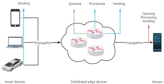
Figure 1. Time delay in the network.

Table 1. Time delay definition in the network.

Name	Definition	Formula
Send Delay	The time taken by a host or router to send a data frame.	$\mathrm{Send}\mathrm{delay}=\frac{\mathrm{length}\mathrm{of}\mathrm{data}\mathrm{frame}\left(\mathrm{b}\right)}{\mathrm{channel}\mathrm{bandwidth}\left(\mathrm{b}/\mathrm{s}\right)}$
Propagation delay	The time it takes for an electromagnetic wave to travel through the channel.	$\mathrm{Propagation}\mathrm{delay}=\frac{\mathrm{channel}\mathrm{length}\left(\mathrm{m}\right)}{\mathrm{propagation}\mathrm{rate}\left(\mathrm{m}/\mathrm{s}\right)}$
Processing delay	The time taken by a host or router to process a received packet.
Queuing delay	The time spent waiting for a packet to be queued in the router’s input queue or output queue.

They are related as in Equation (1):

$$T_{total}=T_{send}+T_{tran}+T_{queu}+T_{proc}$$

(1)

DDoS attack detection via distributed edge devices can take detection that should be done at the server and detect it earlier. This not only relieves the huge pressure on network bandwidth and servers caused by massive amounts of data, but also reduces the propagation latency of the data. By splitting the processing of large-scale traffic through distributed edge devices, the amount of data handled by a single edge device is reduced, which not only reduces the queuing delay of data at a single edge device but also reduces its processing delay and sending delay.

3.1.2. Distributed Computing

Distributed Computing Concepts

Distributed computing is a model of computing that increases computational efficiency and processing power by distributing computational tasks to be executed on multiple computer nodes. In distributed computing, each computing node can perform the same or different tasks, and the nodes communicate and coordinate their work with each other through the network to complete the whole computing task together. Distributed computing can be used for computing tasks in various fields such as processing large-scale data, highly concurrent computing, machine learning, and artificial intelligence. Its advantages include improved computing efficiency, reduced computing costs, enhanced system reliability, and scalability [24]. Distributed computing and centralized computing are related. With the development of the Internet of Things, the scale of data is becoming more and more massive, so the centralized computing of traditional networks can no longer meet the needs of fast computing. Distributed computing, on the other hand, breaks down large amounts of data into many smaller parts, distributes them to multiple nodes for parallel computation and processing, and then merges the results obtained from the computation. This saves overall computation time and improves computation efficiency. This is shown in Figure 2.

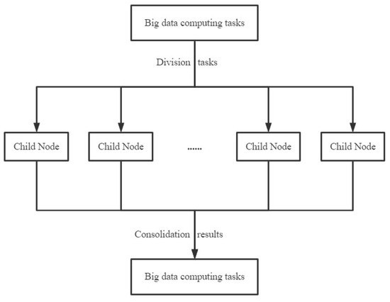
Figure 2. Distributed computing in big data.

Load Balancing for Distributed Computing

How to properly schedule nodes for task assignment is one of the important points of distributed computing. However, some current mainstream systems adopt a random task scheduling strategy that ignores the performance differences of nodes and the state of nodes running, thus easily leading to load inequality and performance degradation [25]. To address these problems, we propose a residual weight random polling algorithm to satisfy the efficient execution of tasks. In Algorithm 1, first, the initial weights of each node are calculated. Then, every time T, the real-time consumption weights of each node are counted, the nodes with residual weights are recorded, and the probability of each node being scheduled is calculated. Finally, the nodes are randomly scheduled according to the probability of each node, and if the scheduled node has no remaining weights to process at that time, this node is removed from the remaining weights queue and randomly scheduled again. The residual weight random polling algorithm not only takes into account the increase or decrease of nodes in the SDN controller cluster and runtime state changes, but also performs cluster state statistics every period T and takes into account the inherent initial performance weight and runtime performance weight of each node. If the node has a stronger initial performance and more residual performance, it is more likely to be scheduled.

Remaining weight of nodes:

$$W_i^{″}=W_i-W_i^{’}$$

(2)

Total remaining weight of nodes:

$$W^{″}={{\displaystyle \sum }}_{i=1}^k{W}_i^{’’}$$

(3)

Node scheduling probability:

$$P_i=\frac{W_i^{’’}}{W^{″}}$$

(4)

$W_i$ the initial weight of the ith node, $W_i^{’}$ the real-time consumption weight of the ith node, $W_i^{’’}$ the remaining weight of the ith node.

Algorithm 1: Remaining weight random polling algorithm.

Input: SDN Controller cluster nodes

Output: Scheduling results

procedure: parameter Optimization

defined Node Initial weight queue weightQue,

for Ni in controller nodes: //Calculate the initial weights of each node

Ni.W = CalculateW(Ni)

add Ni in WQue

while (time = T):

defined:

Node remaining weight queue W′Que,

Node scheduling probability queue PQue,

Total remaining weight of nodes W″=0,

Random scheduling function random()

for Ni in controller nodes: //Iterate through each node of the controller

Ni.W’ = CalculateW′(Ni)

if Ni.W′ < Ni.W then   //If node i has a residual weight

Ni.W″ = Ni.W - Ni.W′

add Ni in weightQue

W″ += Ni.W″ //Total remaining weight of statistical nodes

for Ni in W′Que:

Ni.P = Ni.W″ / W″

add Ni in PQue

resultNode = random (PQue) //Random scheduling of nodes

while (tmpNode ==false) then:

remove tmpNode from PQue

resultNode = random (PQue)

return resultNode

end procedure

3.1.3. SDN

Unlike traditional networks, where switches and routers have integrated control and data planes, SDN separates the control plane from the data plane, allowing network administrators to centrally manage network traffic using software applications. This is shown in Figure 3. The control plane is responsible for determining the best path for network traffic, while the data plane is responsible for forwarding packets. In the SDN architecture, the control plane is decoupled from the data plane and is implemented by a centralized controller. The controller communicates with network devices through standardized protocols such as OpenFlow to manage traffic in the network. One of the key benefits of SDN is that it allows network administrators to manage network traffic more flexibly and dynamically, enabling them to optimize network performance and respond quickly to changing business needs [26]. SDN also provides a centralized view of the network by allowing network administrators to automate network configuration and monitoring tasks, thereby simplifying network management. The SDN network is shown in the figure, and the SDN architecture has four key features: 1. flow-based forwarding. 2. separation of the data level from the control level. 3. located at the data level 4. programmable network.

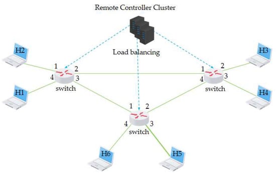
Figure 3. Software defined network architecture.

The core idea of the new network architecture, SDN, is to separate the control level of the network from the data level and to allow the control level to control many of the devices at the data level using the software. In contrast to traditional networks, in the SDN architecture, the routing software in the routers does not exist, as shown in the diagram. As a result, routing information is no longer exchanged between routers at the control level, but is controlled by a logically centralized remote controller, as shown in Figure 4. The SDN remote controller has the following main functions: 1. it keeps track of the state of each host and the network as a whole; 2. the remote controller can calculate the best route for each packet; 3. the remote controller generates its correct forwarding table for each router. A remote controller can physically consist of multiple servers in different locations [27].

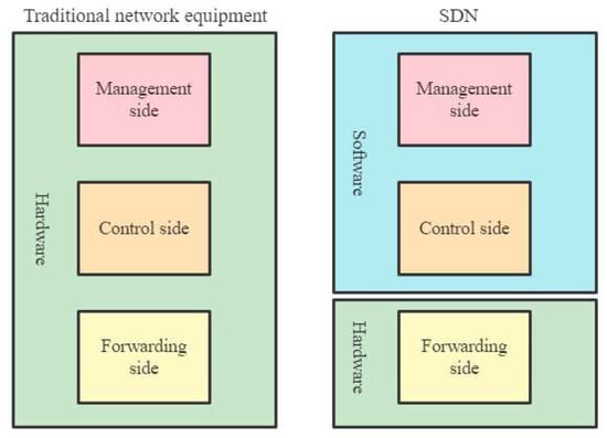
Figure 4. Traditional versus software defined networking.

To cope with the impact of large-scale network traffic that may contain DDoS attacks, this paper introduces the ideas of edge computing and distributed computing, combined with feature selection and machine learning, and proposes an EDRFS framework. This is shown in Figure 5. First, a load balancing algorithm is used to divert the large-scale network traffic from the many edge device switches, and then, the remaining computing power of the SDN controller cluster of edge devices is used to perform DDoS attack detection on the diverted network traffic, realizing the sinking of computing power, distributed parallel computing, reducing data transmission in the cloud, and detecting whether the network traffic contains DDoS attack traffic in real time. The DDoS attack detection part of EDRFS is integrated feature selection combined with RF, which removes redundant features through feature selection to avoid dimensional disasters and reduce prediction time. EDRFS can handle the massive network traffic generated in the era of the Internet of Everything while providing fast and accurate detection of DDoS attacks in real time.

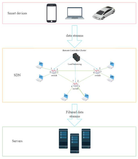
Figure 5. The EDRFS framework proposed in this paper.

3.2. DDoS Attack Detection

3.2.1. Datasets

The CIC-DDoS2019 dataset is a public dataset created by the Canadian Institute for Cyber Security (CIC). The dataset contains data on network traffic from DDoS attacks generated using a variety of attack tools and techniques. The dataset includes 15 scenarios of DDoS attacks, each representing a different combination of attack tools, targets, and victim networks. The attacks are generated in a controlled environment and the network traffic is captured by a set of sensors deployed on the victim’s network. The dataset contains a total of 80 million network flows, including both legitimate and malicious traffic. Each traffic is characterized by 88 features, which include information such as source and destination IP addresses, protocol type, packet size, and duration. The CIC-DDoS2019 dataset is intended to be used for research purposes, such as developing machine learning models for DDoS detection and mitigation. The dataset is available for download from the CIC website and can be used for non-commercial purposes free of charge. As a first choice, we have extracted 82 features from the CICDoS2019 dataset, with a total of 330,000 records, and the dataset contains the latest DDoS attacks. This dataset can simulate the real data flow features to the maximum extent possible, compensating for the shortcomings and limitations of the previous dataset. The dataset was first pre-processed with a series of data type conversions, feature encoding, default value padding, redundant data removal, and data balancing. Then, to unify the magnitudes, the data also need to be normalized. The data are normalized according to equation x, which converts the original data to values in the interval [0,1].

$${\mathrm{x}}_{\mathrm{i}}=\frac{{\mathrm{x}}_{\mathrm{i}}-{\mathrm{x}}_{\min }}{{\mathrm{x}}_{\max }-{\mathrm{x}}_{\min }}$$

(5)

${\mathrm{x}}_{\mathrm{i}}$ is the original data, ${\mathrm{x}}_{\min }$ is the minimum value of that feature data, and ${\mathrm{x}}_{\max }$ is the maximum value of that feature data. Finally, the CIC-DDoS2019 dataset was divided into 67% of the training set for model training and 33% of the test set for model prediction.

3.2.2. Heterogeneous Integration Feature Selection

Feature selection refers to the selection of the most relevant or useful subset of features from the original data. The purpose of feature selection is to improve the accuracy, generalization, interpretability, and computational efficiency of machine learning algorithms. In machine learning, data often contain multiple features, rather than just one feature. Of these features, some may be useful for training and prediction, while others may not contribute to the performance of the algorithm, or may even have a negative impact. A good feature selection algorithm can remove redundant features, reduce noise in the original data, avoid dimensional catastrophe, speed up the learning process later, reduce prediction time, and enable more efficient and accurate learning performance on the simplified dataset. Therefore, the good or bad feature selection directly affects the subsequent model training. Many techniques can be used in feature selection. Some common techniques include filtering methods, packing methods, and embedding methods. Of these, filtering methods select features by calculating the correlation between each feature and the target variable, while packing and embedding methods use the nature of the machine learning algorithm itself to select features. Overall, feature selection is a very important pre-processing step that helps machine learning algorithms to better understand the data and improve the performance of the model. The characteristics of the three feature selection methods are described below.

• Filtered feature selection algorithms

Filtered algorithms are independent of the classifier and use feature selection methods such as distance measures, information measures, and relevance measures to filter the initial features before training the classifier, and then use the filtered features to train the model [28].

2.

Wraparound feature selection algorithm

Wrapped feature selection algorithms are combined with classifiers that directly use the performance of the classifier that will eventually be used as a criterion for evaluating feature subsets, aiming to select a subset of features for a given classifier that can achieve a high accuracy rate in favor of its performance utilizing heuristic or sequential search, etc. [29].

3.

Embedded feature selection algorithms

Unlike filtered and wrapped methods, embedded algorithms do not make a clear distinction between the feature selection process and the classifier training process, but instead integrate the two, automatically performing feature selection during the training of the classifier. Not only does this enable the trained classifier to have a high accuracy rate, but it also results in significant savings in computational overhead [30]. We have combined the characteristics of these three types of feature selection methods and selected five feature selection algorithms. This is shown in Table 2.

Table 2. Feature selection classification.

Classification	Algorithm	Definition
Filter	Variance	Remove features that show the same value for most of them.
	Mutual Information	Reciprocal information measures how much information the presence/absence of a feature has to make a correct prediction for Y.
Wrapper	Backward Elimination	A base model is used to perform multiple rounds of training, sequentially removing non-conforming ones until a certain criterion is met.
Embedded	Lasso(L1)	Lasso regression restricts the model coefficients by adding L1 regularization.
	Random Forest	The generalization of the model is improved by constructing multiple decision trees to reduce the risk of overfitting a single decision tree.

In Algorithm 2, we propose a heterogeneously integrated feature selection algorithm based on these five feature selection algorithms to count features that occur more than three times in the results of these five feature selections.

Algorithm 2: Feature Selection Algorithm.

Input: datasets = DDoS2019 datasets,

featureAlgorithms = [variance(),mutualInformation(),backwardElimination(),lasso(),randomForest()],

model = Random Forest

Output: Feature Results

procedure: Feature Selection

Step 1: defined:

featureResults = [],

featureSet= [1-82],

featureSet1= [],

featureSet2= [],

featureSet3= [],

featureSet4= [],

featureSet5= [],

Step 3: for each featureAlgorithm in featureAlgorithms:

featureSet1=variance(datasets),

eatureSet2=mutualInformation(datasets),

featureSet3=backwardElimination(datasets),

featureSet4=lasso(datasets),

featureSet5=randomForest(datasets)

Step 4: for each feature in [featureSet1, featureSet2, featureSet3, featureSet4, featureSet5]:

++featureSet[feature]

Step 5: for each featureNums in featureSet:

if featureNums ≥ 3 then:

add featureNums.index in featureResults

Step 6: return featureResults

end procedure

3.2.3. Random Forest Optimization

After various machine learning comparisons, we have selected RF as the algorithm for DDoS attack detection. RF, as an integrated learning algorithm, is generated by combining multiple decision tree models. In RF, each decision tree is generated independently and its generation process is based on different random samples and subsets of features. The basic principle of RF is to reduce the risk of overfitting a single decision tree by constructing multiple decision trees, thus improving the generalization ability of the model. Each decision tree in RF is trained on a randomly sampled subset of the original data. RF performs classification or regression by voting or averaging the output of each decision tree [31]. The RF has several important parameters. The most important of these parameters is the sampling rate, the number of decision trees, and the number of features in each decision tree. By tuning these parameters, the accuracy and computational efficiency of RF can be controlled. RF has a wide range of applications in many fields, including finance, healthcare, natural language processing, computer vision, etc. Its advantages include high accuracy, the ability to handle a large number of features and samples, the ability to identify important features, the ability to handle missing data, etc. As shown in Figure 6. The basic process of the RF algorithm is as follows.

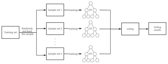
Figure 6. Random forest algorithm flow chart.

• Random sampling: many samples are taken from the original training set using the Bootstrap sampling method (with put-back sampling) as a new training set.
• Random feature selection: a portion of the original feature set is randomly selected as the new feature set, and only this portion of the features is considered when building the decision tree.
• Construction of the decision tree: the decision tree is built based on the new training set and feature set, with each node division being based on a random subset of the feature set.
• Integration of RF: multiple decision trees are generated and eventually each sample is classified or regressed by voting or taking the average.

The RF algorithm has the following advantages.

• RF algorithms are more capable of handling high-dimensional data and large-scale datasets.
• The RF algorithm can effectively avoid the problem of overfitting.
• The RF algorithm can handle both discrete and continuous data.
• The RF algorithm can give the importance ranking of variables, which is a convenient for feature selection.

To further improve the performance of the RF model, we used the DDoS2019 dataset to optimize the main parameters of RF sample, depth, and estimator. The optimization Algorithm 3 is as follows. First, we initialized the RF by setting sample = 0.9, depth = 20, and estimator = 100. First, we set the sampling rate of the RF from 0.1 to 0.9 (step = 0.1) by controlling the variables depth = 20 and estimator = 100 to find the optimal sample in the generated evaluation metrics. Then, with the control variables sample = 0.9, and estimator = 100, set the depth of the RF to increase from 10 to 30 in order (step = 2), and find the optimal depth in the generated evaluation metrics. an estimator from 10 to 210 (step = 20) to find the optimal estimator in the generated evaluation metrics.

Algorithm 3: RF Optimization Algorithm.

Input: DDoS2019 datasets, sample, depth, estimator

Output: Optimized RF

procedure: parameters Optimization

Step 1: defined Indicators = [Acc, Pre, Rec, F1, Ave, Tim]

Step 2: Initialize RF (sample = 0.9, depth = 20, estimator = 100)

Step 2: Xtrain, Xtest, Ytrain, Ytest = split(datasets)

Step 3: Optimise the sample

for i in [0.1,0.2,0.3,0.4,0.5,0.6,0.7,0.8,0.9]:

model = RF (sample = i, depth = 20, estimator = 100)

model.fit

Ypred = model.predict(Xtest)

Indicator = test (Ytest,Ypred )

Indicators.append(Indicator)

Step 4: Select the bestSample with the highest Indicators

Step 5: Optimise depth

for j in range (10,30,2):

model = RF (sample = 0.9, depth=j, estimator = 100)

model.fit

Ypred = model.predict(Xtest)

Indicator = test (Ytest,Ypred )

Indicators.append(Indicator)

Step 6: Select the bestDepth with the highest Indicators

Step 7: Optimise estimator

for k in range (10,210,20):

model = RF (sample = 0.9, depth = 20, estimator = k)

model.fit

Ypred = model.predict(Xtest)

Indicator = test (Ytest,Ypred )

Indicators.append(Indicator)

Step 8: Select the bestEstimator with the highest Indicators

Step 9: return RF (sample = bestSample, depth = bestDepth, estimator = bestEstimator)

end procedure

3.2.4. Evaluation Indicators

Evaluation metrics for machine learning can vary depending on the task and application. The confusion matrix is often used as an evaluation metric for classification problems. As shown in Figure 7. The confusion matrix contains four important classification metrics: True Positive (TP), True Negative (TN), False Positive (FP), and False Negative (FN). The meaning of each of them is shown below. Visualization of the confusion matrix is also one of the common methods used. Data visualization of the confusion matrix can be presented using heat maps or histograms, for example, to provide a more intuitive view of the performance of the classification model [32].

Figure 7. Confusion matrix.

The confusion matrix can be used to calculate many classification evaluation metrics such as accuracy (Acc), precision (Pre), recall (Rec), and F1 values. These evaluation metrics are defined and calculated as shown in Figure 8. In particular, since the F1 value is the summed average containing both accuracy and recall, it can be used to combine the accuracy and recall of the classifier.

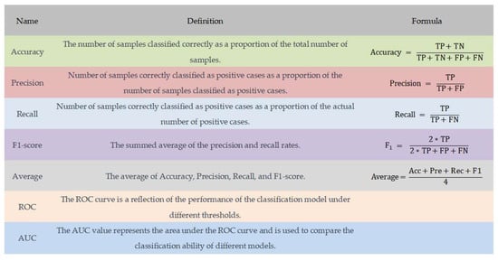
Figure 8. Evaluation indicators.

4. Results and Discussion

To facilitate the calculation and expression, first, we encoded the 82 features extracted from CIC-DDoS2019 features. As shown in Table 3.

Table 3. The 82 features and codes.

Feature	Code	Feature	Code	Feature	Code
Source Port	1	Fwd IAT Min	28	Down/Up Ratio	55
Destination Port	2	Bwd IAT Total	29	Average Packet Size	56
Protocol	3	Bwd IAT Mean	30	Avg Fwd Segment Size	57
Timestamp	4	Bwd IAT Std	31	Avg Bwd Segment Size	58
Flow Duration	5	Bwd IAT Max	32	Fwd Header Length.1	59
Total Fwd Packets	6	Bwd IAT Min	33	Fwd Avg Bytes/Bulk	60
Total Backward Packets	7	Fwd PSH Flags	34	Fwd Avg Packets/Bulk	61
Total Length of Fwd Packets	8	Bwd PSH Flags	35	Fwd Avg Bulk Rate	62
Total Length of Bwd Packets	9	Fwd URG Flags	36	Bwd Avg Bytes/Bulk	63
Fwd Packet Length Max	10	Bwd URG Flags	37	Bwd Avg Packets/Bulk	64
Fwd Packet Length Min	11	Fwd Header Length	38	Bwd Avg Bulk Rate	65
Fwd Packet Length Mean	12	Bwd Header Length	39	Subflow Fwd Packets	66
Fwd Packet Length Std	13	Fwd Packets/s	40	Subflow Fwd Bytes	67
Bwd Packet Length Max	14	Bwd Packets/s	41	Subflow Bwd Packets	68
Bwd Packet Length Min	15	Min Packet Length	42	Subflow Bwd Bytes	69
Bwd Packet Length Mean	16	Max Packet Length	43	Init_Win_bytes_forward	70
Bwd Packet Length Std	17	Packet Length Mean	44	Init_Win_bytes_backward	71
Flow Bytes/s	18	Packet Length Std	45	act_data_pkt_fwd	72
Flow Packets/s	19	Packet Length Variance	46	min_seg_size_forward	73
Flow IAT Mean	20	FIN Flag Count	47	Active Mean	74
Flow IAT Std	21	SYN Flag Count	48	Active Std	75
Flow IAT Max	22	RST Flag Count	49	Active Max	76
Flow IAT Min	23	PSH Flag Count	50	Active Min	77
Fwd IAT Total	24	ACK Flag Count	51	Idle Mean	78
Fwd IAT Mean	25	URG Flag Count	52	Idle Std	79
Fwd IAT Std	26	CWE Flag Count	53	Idle Max	80
Fwd IAT Max	27	ECE Flag Count	54	Idle Min	81
				Inbound	82

In the heterogeneously integrated feature selection algorithm, the output of each feature selection algorithm is shown in Table 4.

Table 4. Results of feature selection.

Type	Algorithm	Feature Code
Filter	Variance	1,2,4,5,6,7,8,10,11,12,18,19,20,21,22,23,28,29, 30,32,38,39,40,41,42,43,44,45,46,56,57,59,66,67,68,70,73,82
	Mutual Information	1,2,4,5,7,8,10,11,12,18,19,20,21,22,39,40,41,42,43,44,56,57,67,68,82
Wrapper	Backward Elimination	1,2,6,31,52,39,42,45,67,70,71,73,82
Embedded	Lasso	23,28,30,31,32,38,39,41,46,59,70,71,77
	Random Forest	1,2,7,8,10,11,12,29,30,32,38,39,41,42,44,45,52,56,57,59,66,68,70,71,73,82

After the heterogeneously integrated feature selection algorithm, the final output is shown in Table 5. Compared to the original 82 features, 24 features remain after the heterogeneously integrated feature selection algorithm, which is a reduction of 58 features compared to the original 82 features.

Table 5. Results of the feature selection algorithm.

Feature	Code	Feature	Code	Feature	Code
Bwd Header Length	39	Fwd Packet Length Max	10	Average Packet Size	56
Destination Port	2	Fwd Packet Length Min	11	Avg Fwd Segment Size	57
Bwd Packets/s	41	Fwd Packet Length Mean	12	Fwd Header Length.1	59
Min Packet Length	42	Bwd IAT Mean	30	Subflow Fwd Bytes	67
Init_Win_bytes_forward	70	Bwd IAT Max	32	Subflow Bwd Packets	68
Inbound	82	Fwd Header Length	38	min_seg_size_forward	73
Total Backward Packets	7	Packet Length Mean	44	Source Port	1
Total Length of Fwd Packets	8	Packet Length Std	45	Init_Win_bytes_backward	71

After feature selection, we conducted experiments on the detection of DDoS attacks on RF under different conditions. The results are shown in Table 6. Experiment 1 (NFS-NRF) was conducted under the following conditions: the DDoS2019 dataset was not selected by the feature selection algorithm, there were 82 features, RF was not optimized by the optimization algorithm, and the test set size was 0.33 million. Experiment 2 (YFS-NRF): the DDoS2019 dataset was selected by the feature selection algorithm, there were 24 features, the RF was not optimized by the optimization algorithm, and the test set size was 0.33 million. The conditions of Experiment 3 (YFS-YRF) were: the DDoS2019 dataset was selected by the feature selection algorithm, there were 24 features, the RF was optimized by the optimization algorithm, and the test set size was 0.33 million. This is based on Table 6 and the corresponding Figure 9 and Figure 10. Comparing the experimental results 1 and 2 shows that, after feature selection, although only 24 features were retained, Acc, Pre, Rec, F1, and Ave did not drop significantly, but the prediction time was reduced by 0.25414 s. The experiments show that the heterogeneously integrated feature selection algorithm can reduce the prediction time by reducing the number of features without reducing the prediction accuracy. Comparing experimental results 2 and 3, it can be seen that the RF optimization algorithm not only reduces the prediction time by 0.016999 s but also improves Acc, Pre, Rec, F1, Ave by 0.084796, 0.007012, 0.095996, 0.053591, 0.060349, respectively. Figure 11 shows the confusion matrix for experiments one, two, and three in that order. Figure 12 shows the ROC curve and AUC values for Experiment 3. The ROC curve is close to the theoretical perfect curve and the AUC value is close to 1. The experiments demonstrate that the RF optimization algorithm can improve the model performance.

Table 6. Performance comparison of experimental results.

Name	Confusion Matrix	Acc	Pre	Rec	F1	Ave	Tim
NFS-NRF	$\begin{array}{cc}18,777& 30\\ 8712& 82,002\end{array}$	0.92018	0.999634	0.903962	0.949394	0.943292	0.688239
YFS-NRF	$\begin{array}{cc}18,227& 580\\ 8712& 82,002\end{array}$	0.915158	0.992977	0.903960	0.946381	0.939619	0.434086
YFS-YRF	$\begin{array}{cc}18,806& 1\\ 4& 90,710\end{array}$	0.999954	0.999989	0.999956	0.999972	0.999968	0.417087

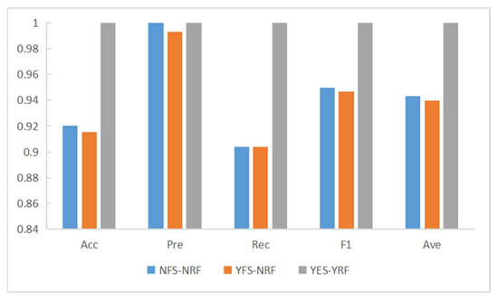
Figure 9. Comparison of experimental results.

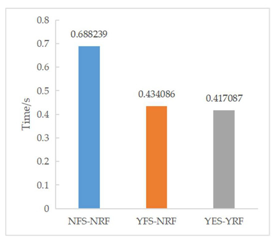
Figure 10. Time for prediction of experimental results.

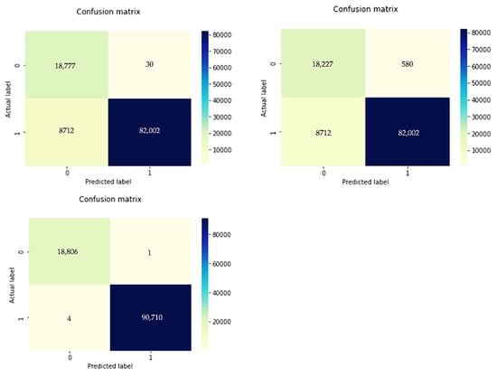
Figure 11. Confusion matrix comparison of experimental results.

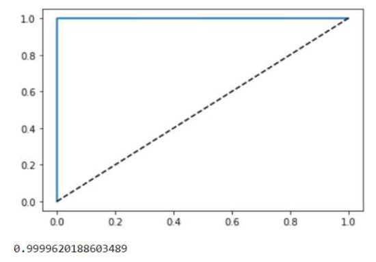
Figure 12. ROC curves and AUC values for Experiment 3 (YFS-YRF).

In a cluster of SDN controllers, when each controller has the same residual weight and the amount of data to be processed is 231,000, the experimental results are shown in Table 7 and Figure 13. As the number of SDN controllers increases, the number of processing tasks for a single controller decreases, and with it, the processing time for the total dataset decreases. The experiments demonstrate the ability of the residual weight random polling algorithm to reduce the processing time of the total tasks using distributed devices.

Table 7. Number of processors and prediction time.

Number of Controllers	1	2	3	4	5	6	7
Number of processors	231,000	198,000	165,000	132,000	99,000	66,000	33,000
Prediction time	0.949209	0.827186	0.695162	0.551112	0.390083	0.268054	0.127017

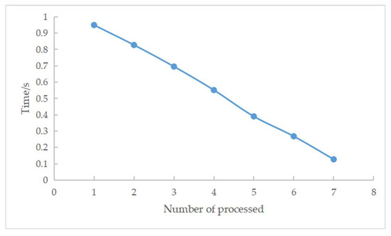
Figure 13. Number of processors and prediction time.

5. Conclusions

In this paper, we combine distributed and edge computing ideas to propose a lightweight framework, EDRFS, to deal with DDoS attacks in SDN networks. To reduce features, avoid dimensional disasters, and reduce prediction time, we integrate Variance, Mutual Information, Backward Elimination, Lasso (L1), and Random Forest feature selection methods to achieve complementary advantages. To improve the accuracy of the RF algorithm for DDoS attack detection, we optimize the main parameters of the RF sample, depth, and estimator. To realize the sinking of computing power, real-time computing in the vicinity, reduce data transmission in the cloud, and lower data propagation delay, we combine the ideas of edge computing and distributed computing, and deploy the DDoS attack detection algorithm on the controller cluster of SDN in a distributed manner, using the remaining computing power of the controller for distributed edge parallel computing. To better schedule nodes and assign tasks, and avoid performance down due to uneven load, we propose a residual weight random polling algorithm to meet the efficient assignment and execution of tasks. The experimental results show that the EDRFS framework proposed in this paper is practical and feasible in terms of accuracy and real-time performance for DDoS attack detection.

References

- Li, S.; Da Xu, L.; Zhao, S. 5G Internet of Things: A survey. J. Ind. Inf. Integr. 2018, 10, 1–9. [Google Scholar] [CrossRef]
- Chica, J.C.C.; Imbachi, J.C.; Vega, J.F.B. Security in SDN: A comprehensive survey. J. Netw. Comput. Appl. 2020, 159, 102595. [Google Scholar] [CrossRef]
- Bawany, N.Z.; Shamsi, J.A.; Salah, K. DDoS Attack Detection and Mitigation Using SDN: Methods, Practices, and Solutions. Arab. J. Sci. Eng. 2017, 42, 425–441. [Google Scholar] [CrossRef]
- Dong, S.; Abbas, K.; Jain, R. A survey on distributed denial of service (DDoS) attacks in SDN and cloud computing environments. IEEE Access 2019, 7, 80813–80828. [Google Scholar] [CrossRef]
- Chen, J.; Ran, X. Deep Learning with Edge Computing: A Review. Proc. IEEE 2019, 107, 1655–1674. [Google Scholar] [CrossRef]
- Cao, K.; Liu, Y.; Meng, G.; Sun, Q. An Overview on Edge Computing Research. IEEE Access 2020, 8, 85714–85728. [Google Scholar] [CrossRef]
- Sun, X.; Ansari, N. EdgeIoT: Mobile Edge Computing for the Internet of Things. IEEE Commun. Mag. 2016, 54, 22–29. [Google Scholar] [CrossRef]
- Ren, Y.; Leng, Y.; Cheng, Y.; Wang, J. Secure data storage based on blockchain and coding in edge computing. Math. Biosci. Eng. 2019, 16, 1874–1892. [Google Scholar] [CrossRef]
- Xiao, Y.; Jia, Y.; Liu, C.; Cheng, X.; Yu, J.; Lv, W. Edge Computing Security: State of the Art and Challenges. Proc. IEEE 2019, 107, 1608–1631. [Google Scholar] [CrossRef]
- Sharma, P.K.; Chen, M.-Y.; Park, J.H. A Software Defined Fog Node Based Distributed Blockchain Cloud Architecture for IoT. IEEE Access 2017, 6, 115–124. [Google Scholar] [CrossRef]
- Birman, K.P. The process group approach to reliable distributed computing. Commun. ACM 1993, 36, 37–53. [Google Scholar] [CrossRef]
- Vavilapalli, V.K.; Murthy, A.C.; Douglas, C.; Agarwal, S.; Konar, M.; Evans, R.; Graves, T.; Lowe, J.; Shah, H.; Seth, S.; et al. Apache Hadoop yarn: Yet another resource negotiator. In Proceedings of the 4th annual Symposium on Cloud Computing, Santa Clara, CA, USA, 1–3 October 2013. [Google Scholar]
- Hindman, B.; Konwinski, A.; Zaharia, M.; Ghodsi, A.; Joseph, A.D.; Katz, R.; Shenker, S.; Stoica, I. Mesos: A platform for fine-grained resource sharing in the data center. In Proceedings of the 8th USENIX Symposium on Networked Systems Design and Implementation, NSDI 2011, Boston, MA, USA, 30 March–1 April 2011; Volume 11. No. 2011. [Google Scholar]
- Alsadie, D. TSMGWO: Optimizing Task Schedule Using Multi-Objectives Grey Wolf Optimizer for Cloud Data Centers. IEEE Access 2021, 9, 37707–37725. [Google Scholar] [CrossRef]
- Arshed, J.U.; Ahmed, M. RACE: Resource Aware Cost-Efficient Scheduler for Cloud Fog Environment. IEEE Access 2021, 9, 65688–65701. [Google Scholar] [CrossRef]
- Banitalebi Dehkordi, A.; Soltanaghaei, M.; Boroujeni, F.Z. DDoS attacks detection through machine learning and statistical methods in SDN. J. Supercomput. 2021, 77, 2383–2415. [Google Scholar] [CrossRef]
- Niyaz, Q.; Sun, W.; Javaid, A.Y. A deep learning based DDoS detection system in software-defined net-working (SDN). arXiv 2016, arXiv:1611.07400. [Google Scholar]
- Erhan, D.; Anarım, E. Istatistiksel Yöntemler Ile DDoS Saldırı Tespiti DDoS Detection Using Statistical Methods. In Proceedings of the 2020 28th Signal Processing and Communications Applications Conference (SIU), Gaziantep, Turkey, 5–7 October 2020. [Google Scholar]
- Tayfour, O.E.; Marsono, M.N. Collaborative detection and mitigation of DDoS in software-defined networks. J. Supercomput. 2021, 77, 13166–13190. [Google Scholar] [CrossRef]
- Yu, Y.; Guo, L.; Liu, Y.; Zheng, J.; Zong, Y. An Efficient SDN-Based DDoS Attack Detection and Rapid Response Platform in Vehicular Networks. IEEE Access 2018, 6, 44570–44579. [Google Scholar] [CrossRef]
- Santos, R.; Souza, D.; Santo, W.; Ribeiro, A.; Moreno, E. Machine learning algorithms to detect DDoS attacks in SDN. Concurr. Comput. Pract. Exp. 2019, 32, e5402. [Google Scholar] [CrossRef]
- Cui, J.; Wang, M.; Luo, Y.; Zhong, H. DDoS detection and defense mechanism based on cognitive-inspired computing in SDN. Future Gener. Comput. Syst. 2019, 97, 275–283. [Google Scholar] [CrossRef]
- Cruz, R.L. A calculus for network delay. II. Network analysis. IEEE Trans. Inf. Theory 1991, 37, 132–141. [Google Scholar] [CrossRef]
- Ben-Or, M.; Goldwasser, S.; Wigderson, A. Completeness theorems for non-cryptographic fault-tolerant distributed computation. In Providing Sound Foundations for Cryptography: On the Work of Shafi Goldwasser and Silvio Micali; Association for Computing Machinery: New York, NY, USA, 2019; pp. 351–371. [Google Scholar]
- Mansouri, N.; Zade, B.M.H.; Javidi, M.M. Hybrid task scheduling strategy for cloud computing by modified particle swarm optimization and fuzzy theory. Comput. Ind. Eng. 2019, 130, 597–633. [Google Scholar] [CrossRef]
- Tan, L.; Pan, Y.; Wu, J.; Zhou, J.; Jiang, H.; Deng, Y. A New Framework for DDoS Attack Detection and Defense in SDN Environment. IEEE Access 2020, 8, 161908–161919. [Google Scholar] [CrossRef]
- Ahmad, S.; Mir, A.H. Scalability, Consistency, Reliability and Security in SDN Controllers: A Survey of Diverse SDN Controllers. J. Netw. Syst. Manag. 2020, 29, 1–59. [Google Scholar] [CrossRef]
- Ghosh, M.; Guha, R.; Sarkar, R.; Abraham, A. A wrapper-filter feature selection technique based on ant colony optimization. Neural Comput. Appl. 2019, 32, 7839–7857. [Google Scholar] [CrossRef]
- Nouri-Moghaddam, B.; Ghazanfari, M.; Fathian, M. A novel multi-objective forest optimization algorithm for wrapper feature selection. Expert Syst. Appl. 2021, 175, 114737. [Google Scholar] [CrossRef]
- Liu, H.; Zhou, M.; Liu, Q. An embedded feature selection method for imbalanced data classification. IEEE/CAA J. Autom. Sin. 2019, 6, 703–715. [Google Scholar] [CrossRef]
- Speiser, J.L.; Miller, M.E.; Tooze, J.; Ip, E. A comparison of random forest variable selection methods for classification prediction modeling. Expert Syst. Appl. 2019, 134, 93–101. [Google Scholar] [CrossRef]
- Luque, A.; Carrasco, A.; Martín, A.; de las Heras, A. The impact of class imbalance in classification performance metrics based on the binary confusion matrix. Pattern Recognit. 2019, 91, 216–231. [Google Scholar] [CrossRef]
Disclaimer/Publisher’s Note: The statements, opinions and data contained in all publications are solely those of the individual author(s) and contributor(s) and not of MDPI and/or the editor(s). MDPI and/or the editor(s) disclaim responsibility for any injury to people or property resulting from any ideas, methods, instructions or products referred to in the content. |
© 2023 by the authors. Licensee MDPI, Basel, Switzerland. This article is an open access article distributed under the terms and conditions of the Creative Commons Attribution (CC BY) license (https://creativecommons.org/licenses/by/4.0/).