A Research on Manipulator-Path Tracking Based on Deep Reinforcement Learning

Abstract

The continuous path of a manipulator is often discretized into a series of independent action poses during path tracking, and the inverse kinematic solution of the manipulator’s poses is computationally challenging and yields inconsistent results. This research suggests a manipulator-route-tracking method employing deep-reinforcement-learning techniques to deal with this problem. The method of this paper takes an end-to-end-learning approach for closed-loop control and eliminates the process of obtaining the inverse answer by converting the path-tracking task into a sequence-decision issue. This paper first explores the feasibility of deep reinforcement learning in tracking the path of the manipulator. After verifying the feasibility, the path tracking of the multi-degree-of-freedom (multi-DOF) manipulator was performed by combining the maximum-entropy deep-reinforcement-learning algorithm. The experimental findings demonstrate that the approach performs well in manipulator-path tracking, avoids the need for an inverse kinematic solution and a dynamics model, and is capable of performing manipulator-tracking control in continuous space. As a result, this paper proposes that the method presented is of great significance for research on manipulator-path tracking.

1. Introduction

A manipulator is a highly integrated mechanical system combined with electromechanical control. It is a typical time-varying and highly coupled multi-input, multi-output nonlinear system. Its regulation is extremely difficult because it is a complex system with several uncertainties. Researchers have studied manipulator-control techniques extensively over the past few decades. The existing control methods for robots include computational torque control, robust adaptive control [1], adaptive neural-network control [2], output-feedback control [3,4], dead-zone nonlinear compensation control [5], virtual decomposition control [6], the sliding mode controller [7] and so on.

The subject of path tracking [8,9] is crucial to manipulator control. The challenge is to determine how to ensure that the manipulator’s end follows the optimal path after the path-planning algorithm has successfully planned an optimal path. According to Cai ZX [10], each manipulator joint’s acceleration and speed are broken out separately. Through position or speed feedback, they modify the target speed or desired acceleration of each joint and use the error as a control input. It is challenging to accurately determine the dynamic characteristics of each manipulator link because the end effector frequently clamps various objects during actual manipulator control. The track and control of the manipulator are simultaneously made challenging by the presence of external interference and flaws in the dynamic modeling. In order to maintain the unknown components within a certain range and to account for the disparity between the predicted model and the real model of the manipulator, Spong [11] introduced a robust term to the control input. In order to increase the resilience and stability of the tracking and compensate for the error created by the external disturbance and the linearization of the dynamic model, Purwar [12] optimized the parameters of the neural-network controller using the Lyapunov stability criterion. To prevent collisions with objects in the workspace and irregular robot configurations, Jasour [13] presented nonlinear-model predictive control (NMPC), which allows the end effectors of the robot manipulator to follow preset geometric routes in Cartesian space. The robot’s nonlinear dynamics, including the dynamics of the actuator, are also taken into account. Chen [14] presented an intelligent control approach that combines sliding mode control (SMC) and fuzzy neural networks (FNN) to accomplish backstepping control for manipulator-path tracking problem. Zhang [15] introduced the concept of the virtual rate of change of torque and virtual voltage, which are linear relationships in the state and control variables. In order to improve the motion accuracy, he added kinetic constraints and transformed the non-convex minimum-time route-tracking problem into a convex optimization problem that can be solved quickly.

The processes of exact dynamic modeling and inverse kinematics solutions are used in all of the methods mentioned above. However, as the manipulator’s degree of freedom increases, the complexity of the dynamic modeling and the number of inverse kinematics solution calculations increase, and the inverse solution is not singular. All these approaches have restrictions in terms of how they can be used [16,17]. Path-tracking issues can now be solved without the need for system-dynamics modeling thanks to a number of recent successful applications of reinforcement learning to decision-control problems. This opens up new perspectives on path-tracking issues. The manipulator-path-tracking problem can be modeled as a Markov decision process (MDP) using the reinforcement learning [18,19] approach, which interacts with samples to optimize the control policy. Guo [20] completed the path tracking of the UR5 manipulator using the depth-value-function approach (DQN). The action space is discretized, however, and it is challenging to finely control the manipulator. For managing robots with unknown parameters and dead zones, Hu [21] offered a deep-reinforcement-learning system. Three components make up the algorithm: a state network that estimates information about the robot manipulator’s state; a proposed critic network that assesses the effectiveness of the network; and an action network that learns a method for enhancing the performance metrics. Liu [22] achieved tracking control over a manipulator in a continuous action space, but the algorithm’s learning process was unstable and was heavily influenced by even minor changes to the hyperparameters. There is currently no deep-reinforcement-learning system that can reliably and continuously control the manipulator for route-tracking operations, according to the research findings.

To address the aforementioned issues, this paper proposes a reinforcement-learning method for multi-DOF manipulator-path tracking, which converts the tracking-accuracy requirements and energy constraints into cumulative rewards obtained by the control strategy to ensure the stability and control accuracy of the tracking trajectory. The entropy of the policy is used as an auxiliary gain of the agent and introduced into the training process of the control strategy, thereby increasing the robustness of the path tracking. The method has good results in manipulator-path tracking, which not only avoids the process of finding the inverse kinematic solution, but also does not require a dynamics model and can ensure control over the tracking of the manipulator in continuous space.

The remainder of this essay is structured as follows. The theoretical foundation of the algorithms in this paper, as well as the specific algorithmic applications and simulated experimental settings corresponding to the three manipulators, are presented in Section 2 after an introduction to the theoretical knowledge of deep-reinforcement-learning algorithms. The findings of the three manipulators’ simulation experiments are mostly shown in Section 3. The simulation results are analyzed in Section 4, along with the algorithm used in this paper in comparison to other algorithms. The work is concluded in Section 5, which also identifies potential future research areas.

2. Method

2.1. Deep Q Network

The value-function approach in deep reinforcement learning, which originally evolved from the Q-Learning algorithm in classical reinforcement learning, is the basis of the Deep Q-Network (DQN) algorithm [23], a classic algorithm. The algorithm known as Q-Learning [24] is based on the $Q$ value, which is the projected future cumulative reward value of action $a$ (activity a must be finite and discrete), taken in accordance with policy $\pi$ in state $S$.

$$Q_{\pi }\left(s,a\right)={{\rm E}}_{\pi }\left[{\displaystyle \sum _{t=0}{\gamma }^{t}r\left(s_t,a_t\right)}|s_0=s,a_0=a\right]$$

(1)

In Equation (1), $\gamma$ is the discount factor determining the agent’s horizon. The optimal value $Q^{\ast }$ is defined as the maximized $Q$ value, and the strategy that can obtain the optimal value is defined as the optimal strategy ${\pi }^{\ast }$. The DQN uses a deep neural network $Q_{\pi }\left(s,a;\theta \right)$ with parameters $\theta$ to replace the $Q$ value $Q_{\pi }\left(s,a\right)$, which allows the algorithm to remain valid in the case of high-dimensional and continuous input states $S$. In addition, the experience-playback pool Replay buffer and a target Q network with parameters ${\theta }^{\prime }$ are also added to DQN. The Replay buffer improves the utilization efficiency of samples, and the use of the target Q network solves the loss in the neural-network-function problem. The target Q network is defined as Equation (2).

$$y=r+\gamma \underset{a^{\prime }}{\max }Q\left(s^{\prime },a^{\prime };{\theta }^{\prime }\right)$$

(2)

Therefore, this problem can be transformed into a supervised learning problem to solve, that is, $\underset{\theta }{\mathit{min}}\sum \left(y-Q\left(s,a;\theta \right)\right)$, where $\theta$ in ever $\tau$ step copy their own parameters to ${\theta }^{\prime }$.

2.2. Soft Actor-Critic

Although the DQN algorithm, which is a milestone in deep reinforcement learning, solves the problem of high-dimensional and continuous input states, which cannot be solved by classical reinforcement learning, it still cannot solve situations in which the output actions are high-dimensional and continuous (such as multi-degree-of-freedom manipulator). Although the other deep-reinforcement-learning algorithms (such as DDPG [25], TD3 [26], and other algorithms) can handle cases in which the output action is high-dimensional and continuous, they usually have high sample complexity and weak sample convergence, which lead to some additional hyperparameter tuning.

The Soft Actor-Critic (SAC) algorithm [27,28] is a reinforcement-learning algorithm that introduces the maximum-entropy theory. In the framework of the algorithm, the strategy not only needs to maximize the expected cumulative reward value, but also needs to maximize the expected entropy, as shown in Equation (3),

$${\pi }^{*}=\max {\displaystyle \sum _{t=0}^T{E}_{(s_t,a_t)~p_{\pi }}[r(s_t,a_t)+\alpha H(\pi (\cdot |s_t))]}$$

(3)

where $\alpha$ is the weight of the entropy term, which can determine the relative importance of the entropy term relative to the reward term, thereby controlling the randomness of the optimal strategy.

The maximum-entropy framework uses a technique called “Soft Policy Iteration” to alternately evaluate and improve policies in order to accomplish this goal. In an environment where the state space is discrete, the method can obtain the soft $Q$ value from the randomly initialized function $Q:S\times A\to R$ and repeatedly apply the modified Bellman backup operator $T^{\pi }$, as shown in Equation (4),

$$T^{\pi }Q(s_t,a_t)=r(s_t,a_t)+\gamma E_{s_{t+1:p}}[V(s_{t+1})]$$

(4)

where

$$V(s_t)=E_{a_t~\pi }[Q(s_t,a_t)-\log \pi (a_t|s_t)]$$

(5)

is the soft state-value function used to calculate the policy value in policy evaluation. In the continuous state, a neural network with parameters is first used to replace the soft Q-function $Q_{\theta }\left(s_t, a_t\right)$, and then it is trained to minimize the Bellman residual, as shown in Equation (6),

$$J_Q(\theta )=E_{(s_t,a_t)~D}\left[\frac{1}{2}{\left(Q_{\theta }(s_t,a_t)-\left(r(s_t,a_t)+\gamma E_{s_{t+1}~p}[V_{\overline{\theta }}(s_{t+1})]\right)\right)}^2\right]$$

(6)

which can also be optimized with stochastic gradients:

$${\stackrel{\wedge }{{\displaystyle \nabla }}}_{\theta }{J}_Q(\theta )={{\displaystyle \nabla }}_{\theta }{{\displaystyle Q}}_{\theta }(s_t,a_t)\left({{\displaystyle Q}}_{\theta }\right.(s_t,a_t)-r(s_t,a_t)-\left.\gamma {{\displaystyle V}}_{\overline{\theta }}(s_{t+1})\right)$$

(7)

where $V_{\overline{\theta }}\left(s_{t+1}\right)$ is estimated by the target network of Q and the Monte Carlo estimation of the soft state-value function sampled from the experience pool.

The goal of policy improvement is to maximize the available reward, so the policy must be updated to the new soft Q function’s exponential form and restricted to a parameterized distribution (such as the Gaussian distribution). The policy must then be projected back into the permissible policy space using an information projection defined in terms of the Kullback–Leibler (KL) divergence, as displayed in Equation (8),

$${\pi }_{new}=\arg \underset{{\pi }^{\prime }\in \mathsf{\Pi }}{\min }{D}_{KL}\left({\pi }^{\prime }(\cdot |s_t)\mathrm{P}\frac{\exp (Q^{{\pi }_{old}}(s_t,\cdot ))}{Z^{{\pi }_{old}}(s_t)}\right)$$

(8)

where $Z^{{\pi }_{old}}\left(s_t\right)$ can be ignored because it has no effect on the gradient. Furthermore, the policy ${\pi }_{\varphi }\left(a_t|s_t\right)$ is parameterized with a neural network that can output mean and variance to define a Gaussian distribution, and then the parameters of the policy are learned by minimizing the expected KL divergence, as shown in Equation (9).

$$J_{\pi }\left(\varphi \right)=E_{s_t~D}\left[E_{a_t~{\pi }_{\varphi }}\left[\log {\pi }_{\varphi }(a_t|s_t)-Q_{\theta }(s_t,a_t)\right]\right]$$

(9)

However, since it is difficult to find the gradient in the Gaussian distribution $a~N\left(m,s\right)$, it is converted into a form in which the gradient is easy to find: $a=m+s\epsilon$, $\epsilon ~N\left(0, 1\right)$, i.e., $a_t=f_{\varphi }\left({\epsilon }_t,s_t\right)$. The policy network can then be optimized by applying the policy gradient to the expected future reward, as shown in Equation (10).

$$J_{\pi }\left(\varphi \right)=E_{s_t~D,{\epsilon }_t~N}\left[\log {\pi }_{\varphi }(f_{\varphi }({\epsilon }_t;s_t)|s_t)-Q_{\theta }(s_t,f_{\varphi }({\epsilon }_t;s_t))\right]$$

(10)

This paper can also approximate the gradient of Equation (10) with:

$${\stackrel{\wedge }{\nabla }}_{\varphi }{J}_{\pi }\left(\varphi \right)={\nabla }_{\varphi }\log {\pi }_{\varphi }(a_t|s_t)+({\nabla }_{a_t}\log {\pi }_{\varphi }(a_t|s_t)-{\nabla }_{a_t}Q(a_t|s_t)){\nabla }_{\varphi }{f}_{\varphi }({\epsilon }_t;s_t)$$

(11)

2.3. Deep-Reinforcement-Learning Algorithm Combined with Manipulator

This paper models the path-tracking problem of manipulator as a Markov decision process (MDP), which is represented by $<S, A, R, T, \gamma >$, where $s_t\in S$ represents the observations of the agent. The policy $\mathsf{\Pi }:S\to A$ maps the current environmental state $s_t$ to the control input $a_t\in A$ of each joint of the manipulator, $T\left(s_{t+1}|s_t, a_t\right)$ represents the dynamic characteristics of the robotic arm, that is, the probability that the system transitions from state $s_t$ to $s_{t+1}$ under the control of $a_t$. The expected path $P^{\ast }\in {\mathbb{R}}^{N\times 3}$ of the manipulator can be generated by traditional path-planning methods, where N is the number of points on the path. The instantaneous reward obtained by the agent at time $t$ is represented by $r_t\in R$, which is related to the tracking accuracy of the robot arm on the desired path and the energy consumed. The policy continuously interacts with the manipulator system to obtain the sampling trajectory $\tau =\left\{s_0,a_0,\cdots ,s_t,a_t, \cdots ,s_T,a_T\right\}$. The objective of reinforcement learning is to maximize the expected cumulative reward that the agent receives, as illustrated in Equation (12).

$$\underset{}{{\mathrm{maximize}}_{\pi \in \prod }}{{\rm E}}_{\tau ~p\left(\tau \right)}\left[{\displaystyle \sum _{t=0}^T{\gamma }^{t}r\left(s_t,a_t\right)}\right]$$

(12)

where

$$p\left(\tau \right)=p\left(s_0\right){\displaystyle \prod _{t=0}^T\pi \left(a_t|s_t\right)T\left(s_{t+1}|s_t,a_t\right)}$$

(13)

Figure 1 depicts the framework of the deep-reinforcement-learning-based robot-arm path-tracking model. The framework is made up of the manipulator body, the desired path, the control strategy, and the feedback controller. The tracking error of the desired path minus the actual path of the manipulator is the input signal. The input signal used by the control strategy to determine the anticipated position and speed of each joint at the following instant serves as the reference signal for the feedback controller. The feedback controller combines each joint’s current position and velocity data and produces the necessary joint torque to move the manipulator’s end point, thereby performing the path-tracking function.

This appealing framework was applied to two-link manipulator, multi-degree-of-freedom manipulators and redundant manipulators to test path tracing in the V-REP PRO EDU 3.6.0 simulation platform.

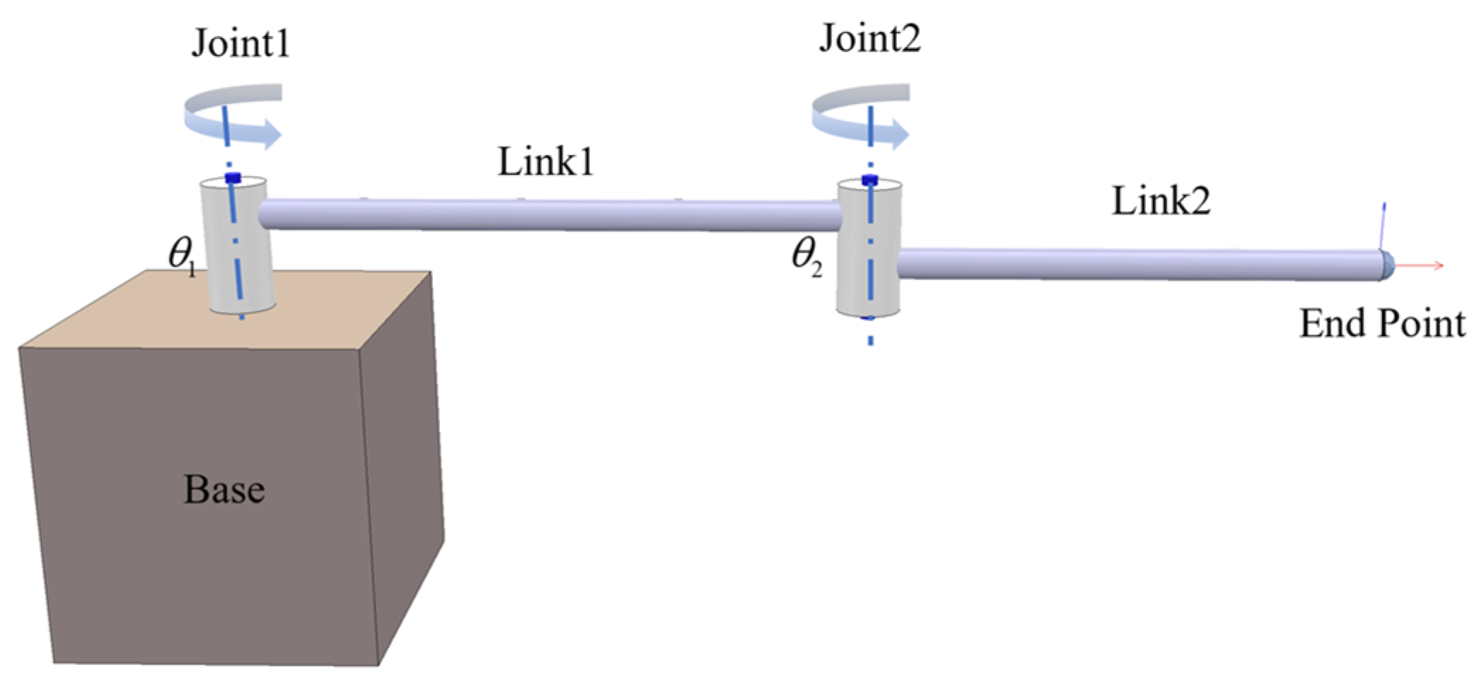
2.3.1. Application of Two-Link Manipulator

The plane of two-link manipulator simulation system is shown in Figure 2. The settings of the two-link manipulator in the simulation environment are as follows. The lengths of the rods are $l_1=1.0 \mathrm{m}, l_2=0.8 \mathrm{m}$, and the mass of the rods are $m_1=0.1 \mathrm{k}\mathrm{g}, m_2=0.08 \mathrm{k}\mathrm{g}$. Each joint adopts the incremental control method, that is, the joint rotates around a fixed angle $\left|\mathsf{\Delta }\theta \right|$ in the direction given by the control signal $a_t$ at any time $t$, where $a_t≔\left[{\mathsf{\Delta }\theta }_t^1,{\mathsf{\Delta }\theta }_t^2\right]\in {\mathbb{R}}^2$,$\left|∆{\theta }_t^i\right|={0.05}^{°}, i=1, 2$. The state of the entire simulation system is $s_t≔\left[{\theta }_t^1, {\theta }_t^2 , {\dot{\theta }}_t^1 , {\dot{\theta }}_t^2 ,x_t ,y_t ,x_t^{\ast } ,y_t^{\ast }\right]\in {\mathbb{R}}^8$, where ${\theta }_t^i,{\dot{\theta }}_t^i$ are the angle and angular velocity of each joint at $i$th time. The $\left(x_t,{ y}_t\right)$ is the position of the endpoint of the manipulator at time $t$, and the desired target-point position $\left(x_t^{\ast },{ y}_t^{\ast }\right)$ is set as Equation (14).

$$\begin{array}{c}\left\{\begin{array}{c}{x}_t^{*}=l_2\cos \left({\omega }_{1}t+{\omega }_{2}t\right)+l_1\cos \left({\omega }_{1}t\right)\\ y_t^{*}=l_2\sin \left({\omega }_{1}t+{\omega }_{2}t\right)+l_1\sin \left({\omega }_{1}t\right)\end{array}\right.\end{array},\hspace{1em}{\omega }_1={\omega }_2=1 \mathrm{rad}/\mathrm{s}$$

(14)

The two-link manipulator’s output action has low dimensionality and can be approximated as a discrete quantity, so the algorithm uses the classical DQN algorithm. The strategy’s network structure in the DQN algorithm is as follows: the input state is 8-dimensional, the output action is 2-dimensional, the hidden layer has two layers, and the number of nodes in each layer is 50. The hyperparameters are set as follows: replay buffer = 1 × 10⁶, learning rate = 3 × 10⁻⁴, discount factor = 0.99, batch-size = 64, the update between the Q network and the target Q network adopts the soft update method, and its soft parameter tau = 0.001. In addition, the setting of the reward is $r_t=\mathit{exp}\left(-\left|p_t^{\ast }-p_t\right|\right)$, where $p_t^{\ast }, p_t$ are the target path points at time t and the position of the end point of the robot arm, respectively.

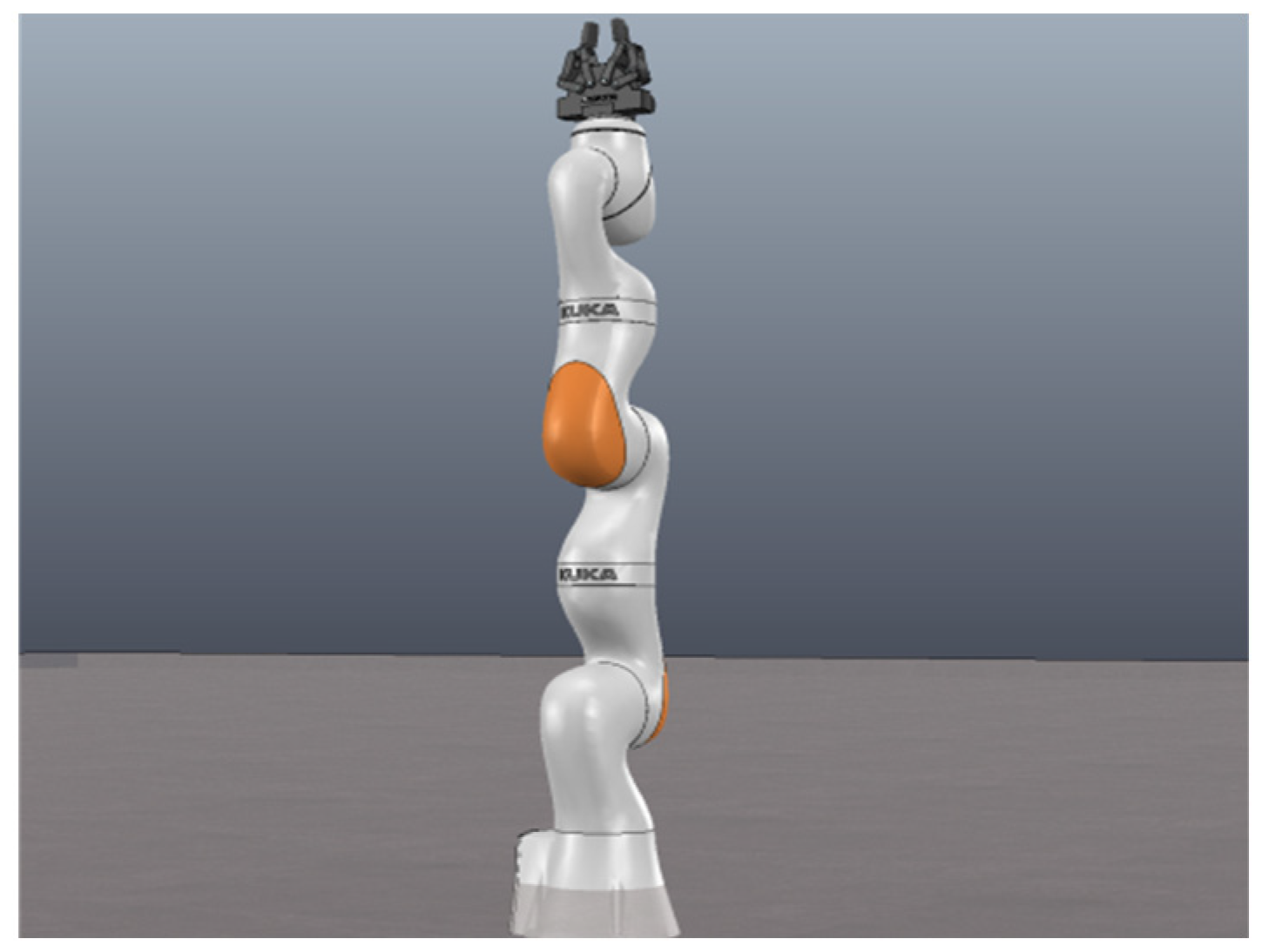
2.3.2. Application of Multi-Degree-of-Freedom Manipulator

This paper applies the algorithm to a multi-degree-of-freedom manipulator, UR5, to achieve path tracking under continuous control. The UR5 simulation system, which is shown in Figure 3, uses a deep-reinforcement-learning algorithm to achieve path tracking in the presence of obstacles after generating a path by a conventional path-generation algorithm. The system’s actions $a≔\left[a_1, a_2, a_3,{ a}_4,{ a}_5,{ a}_6,\right]\in {\mathbb{R}}^6$, and states are set as $s≔\left[{\theta }_1, {\theta }_2, {\theta }_3, {\theta }_4, {\theta }_5, {\theta }_6, {\dot{\theta }}_1, {\dot{\theta }}_2, {\dot{\theta }}_3, {\dot{\theta }}_4, {\dot{\theta }}_5, {\dot{\theta }}_6, ∆x, ∆y, ∆z\right]\in {\mathbb{R}}^{15}$, where ${\theta }_i, {\dot{\theta }}_i$ is the angle and angular velocity of the first joint, and $∆x, ∆y, ∆z$ are the distance between the endpoints p and the corresponding desired target points $p^{\ast }$. The initial position of the endpoint is [−0.095, −0.160, 0.892] and the initial position of the target point is [−0.386, 0.458, 0.495]. The desired path is generated by the traditional RRT [1,29] path-generation algorithm with the stride set to 100.

In addition, this experiment set up 4 additional variables to explore the impact of these factors on tracking performance:

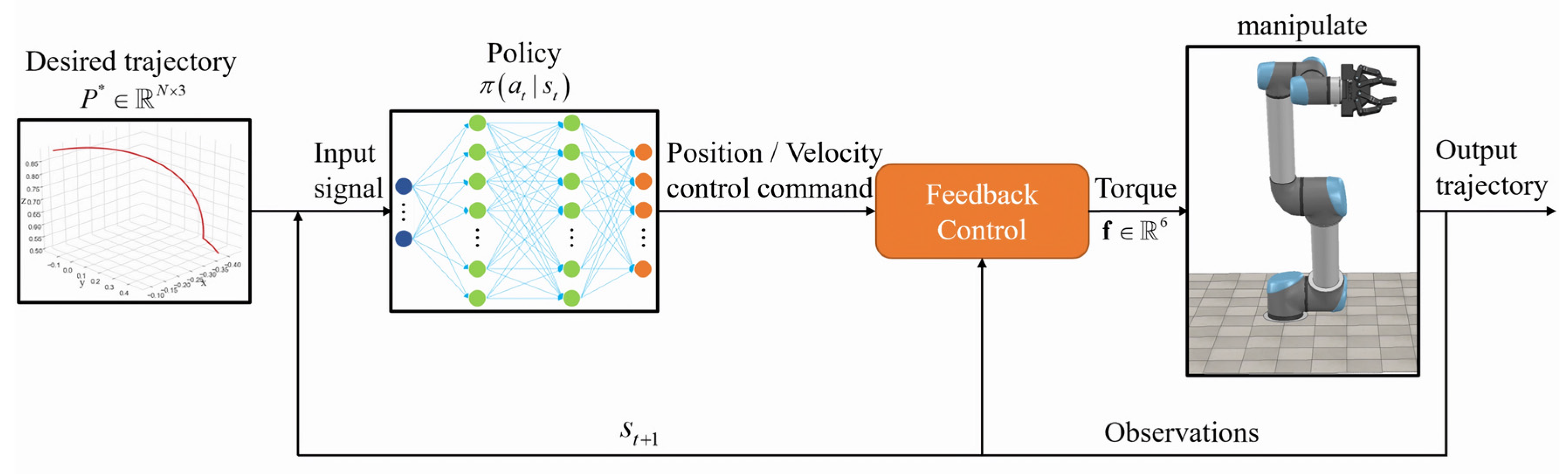
• The upper control method of the manipulator adopts two control methods, position control and velocity control. The position control is the control of the joint angle, and the input action is the increment of the joint angle. The range of the increment at each moment is set as [−0.05, 0.05] rad. The velocity control is the control of joint angular velocity. The input action is the increment of joint angular velocity. The increment range of each moment was set to [−0.8, 0.8] rad/s in the experiment. In addition, the underlying control of the manipulator adopts the traditional PID torque-control algorithm.
• Addition of noise to the observations. This paper set up two groups of control experiments, one of which added random noise to the observations; the noise was adopted from the standard normal distribution N(0,1), and the size was 0.005 × N(0,1).
• The setting of the time-interval distance $n$. The target path points given by the manipulator at every n time are the target path points at the N*$n$ time, where N = 1, 2, 3…, and are used to study the effect of different interval points on the tracking results. In the experiments, the interval distances were set as 1, 5, and 10, respectively.
• Terminal reward. A control experiment was set up in which, during the training process, when the distance between the endpoint of the robotic arm and the target point was within 0.05 m (the termination condition is met), an additional +5 reward was given to study its impact on the tracking results.

In order to improve sampling efficiency, the SAC algorithm combines the value-based and policy-based approaches, using the value-based approach to learn the Q-value function or state-value function V and the policy-based approach to learn the policy function, thus making it suitable for the continuous high-dimensional action space and, therefore, more appropriate for control over tracking of the manipulator. As a result, the SAC algorithm was chosen to control tracking of the multi-degree-of-freedom manipulator in this research. All network structures were as follows: each network contained two hidden layers, the number of nodes in each layer was 200, and the activation function of the hidden layer was set to ReLu. The hyperparameters were set as follows: replay buffer = 1 × 10⁶, discount factor = 0.99, batch size = 128, the update between the Q network and the target Q network adopted the soft update method, the soft parameter tau = 0.01, the learning rate of Actor and Critic network were both set to learning rate = 1 × 10⁻³, and the weight coefficient of policy entropy during the entire training process $\alpha$ = 1 × 10⁻³. The reward settings for this experiment were set as Equation (15).

$$r_t=-‖p_{\tau \left(t,n\right)}^{*}-p_t‖\hspace{1em},\hspace{1em}\begin{array}{c}\tau \left(t,n\right)=\left\{\begin{array}{cc}n\left(\mathrm{floor}\left(t/n\right)+1\right)& n>1\\ t& n=1\end{array}\right.\end{array}$$

(15)

where $n$ is the interval distance. In addition, an experiment was terminated when the robot arm ran for 100 steps or the distance between the end point of the robot arm and the target point was within 0.05 m.

2.3.3. Application of Redundant Manipulator

The algorithm proposed in this paper was also applied on a 7-degree-of-freedom redundant manipulator for path tracking. The simulation system of the 7-DOF redundant manipulator is shown in Figure 4. The simulation platform still used V-REP PRO EDU 3.6.0, and the simulated manipulator used the KUKA LBR ii wa 7 R800 redundant manipulator. The setting of actions was $a≔\left[a_1, a_2, a_3,{ a}_4,{ a}_5,{ a}_6,{ a}_7\right]\in {\mathbb{R}}^7$, and states were set as $s≔\left[{\theta }_1, {\theta }_2, { \theta }_3, { \theta }_4, {\theta }_5, {\theta }_6, {\theta }_7, {\dot{\theta }}_1, {\dot{\theta }}_2, {\dot{\theta }}_3, {\dot{\theta }}_4, {\dot{\theta }}_5, {\dot{\theta }}_6, {\dot{\theta }}_7, ∆x, ∆y, ∆z\right]\in {\mathbb{R}}^{17}$ where ${\theta }_i, {\dot{\theta }}_i$ is the angle and angular velocity of the first joint and $∆x, ∆y, ∆z$ is the distance between the end-point $p$ of the manipulator and the corresponding desired target point $p^{\mathrm{*}}$. The initial position of the end-point was [0.0044, 0.0001, 1.1743], and the initial position of the target point was [0.0193, 0.4008, 0.6715]. The expected path was an arc trajectory generated by the path-generation algorithm, and the step size was set to 50.

The setup of the redundant-manipulator path-tracking experiment was exactly the same as that of UR5. The experiment still used the continuous-control reinforcement-learning algorithm SAC, and all network structures were also the same as in the UR5 setup. That is, each network contained two hidden layers, the number of nodes in each layer was 200, and the activation function of the hidden layer was set to ReLu. The hyperparameter settings were also the same: replay buffer = 1 × 10⁶, discount factor = 0.99, batch size = 128, the update between the Q network and the target Q network adopts the soft update method, the soft parameter tau = 0.01, the learning rate of Actor and Critic network are both set to learning-rate = 1 × 10⁻³, and the weight coefficient α = 1 × 10⁻³ of policy entropy during the whole training process.

The reward settings were also the same as those used before. The only difference was that the redundant-manipulator path tracking-experiment was conducted to verify the generalization of the algorithm, so it did not involve the results when other hyperparameter conditions changed. Therefore, the default separation distance in the reward setting was $n$= 1.

3. Simulation Results

In this section, the simulation results of path tracking of three manipulators are compared and analyzed.

3.1. Simulation Results of Planar Two-Link Manipulator

The two-link manipulator experiment was mainly used to verify the feasibility of the reinforcement-learning algorithm in the field of manipulator-path tracking. The specific parameter settings for the experiment are detailed in Section 2.3.1. The tracking-curve results of this experiment are shown in Figure 5.

The blue line represents the real operating end path, while the red line represents the desired-goal path. The tracking findings in Figure 5 show that the deep-reinforcement-learning-based strategy completely succeeds in tracking the target path. The experimental findings in the simulation environment are displayed in Figure 6.

The experimental results show that it is completely feasible to use the deep-reinforcement-learning algorithm to achieve path tracking with a simple two-link manipulator.

3.2. Simulation Results of Multi-Degree-of-Freedom Manipulator

After exploring the application of reinforcement learning in path tracking, as well as its successful application to the two-link manipulator to achieve the tracking target, the application of the multi-degree-of-freedom manipulator UR5 to conduct path tracking under continuous control was also explored. The specific parameter settings for the experiment are detailed in Section 2.3.2.

The experimental results are shown in the following figures. Figure 7a,b show the path-tracking results without observation noise and with observation noise in the position-control mode, respectively. Figure 7c,d show the speed-control results and the path-tracking results with and without observation noise in the mode, respectively. Different time intervals are set in each picture; the upper three curves of each picture are the results of not giving the terminal reward, and the lower three curves are the results of giving the terminal reward.

In addition, this experiment also quantitatively analyzed the tracking results, calculated the average error between the obtained path and the target path under different experimental conditions and the average distance between the endpoint of the manipulator and the target point at the last moment, and set the average error to less than 0.07 and the error of the target point to less than 0.05 to achieve the tracking-accuracy requirements. The results are shown in

Table 1. Results of position-control-mode path tracking.

Position Control		w/o Observation-Noise			Observation-Noise
		Interval			Interval
		1	5	10	1	5	10
Average error between tracks (m)	w/o terminal reward	0.0374	0.0330	0.0592	0.0394	0.0427	0.0784
	terminal reward	0.0335	0.0796	0.0502	0.0335	0.0475	0.0596
Distance between end points (m)	w/o terminal reward	0.0401	0.0633	0.0420	0.0443	0.0485	0.0292
	terminal reward	0.0316	0.0223	0.0231	0.0111	0.0148	0.0139

and

Table 2. Results of velocity-control-mode path tracking.

Velocity Control		w/o Observation-Noise			Observation-Noise
		Interval			Interval
		1	5	10	1	5	10
Average error between tracks(m)	w/o terminal reward	0.0343	0.0359	0.0646	0.0348	0.0318	0.0811
	terminal reward	0.0283	0.0569	0.0616	0.0350	0.0645	0.0605
Distance between end points (m)	w/o terminal reward	0.0233	0.0224	0.0521	0.0456	0.0365	0.0671
	terminal reward	0.0083	0.0030	0.0337	0.0275	0.0192	0.0197

.

The training-process curve is shown in Figure 8, where (a) is the training-process curve without observation noise in position-control mode, (b) is the training-process curve with the addition of observation noise in position-control mode, (c) is the training-process curve without observation noise in velocity-control mode, and (d) is the training-process curve with the addition of observation noise in velocity-control mode. The X-axis represents the number of training sessions and the Y-axis represents the reward value set in the reinforcement learning. There are six curves in each graph, which represent the training curves with different time intervals with or without terminal reward. The training curves that reach a reward value of 0 on each graph are those with the terminal reward added.

In addition, since the system-dynamics model is not considered in the path-tracking experiment based on deep reinforcement learning, in order to verify the advantage of the method based on deep reinforcement learning without the need for the dynamic model, this paper further explores the influence of the change in dynamic characteristics in the experimental results. To this end, we changed the quality of the end effector, the trained model was tested, and the experimental results are shown in

Table 3. Analysis of dynamic characteristics of position control.

Position Control			0.5 kg	1 kg	2 kg	3 kg	5 kg
Average error between tracks (m)	w/o observation noise	w/o terminal reward	0.03742	0.03743	0.03744	0.03745	0.03746
		terminal reward	0.03354	0.03354	0.03359	0.03355	0.03355
	observation noise	w/o terminal reward	0.03943	0.03943	0.03943	0.03942	0.03941
		terminal reward	0.03346	0.03346	0.03346	0.03346	0.03345
Distance between end points (m)	w/o observation noise	w/o terminal reward	0.04047	0.04047	0.04048	0.04049	0.04050
		terminal reward	0.03165	0.03166	0.03157	0.03159	0.03161
	observation noise	w/o terminal reward	0.04430	0.04441	0.04438	0.04430	0.04436
		terminal reward	0.01110	0.01109	0.01109	0.01108	0.01105

and

Table 4. Analysis of Dynamic Characteristics of Velocity Control.

Velocity Control			0.5 kg	1 kg	2 kg	3 kg	5 kg
Average error between tracks (m)	w/o observation noise	w/o terminal reward	0.03426	0.03427	0.03425	0.03426	0.03425
		terminal reward	0.02826	0.02825	0.02866	0.02873	0.02882
	observation noise	w/o terminal reward	0.03478	0.03479	0.03483	0.03486	0.03497
		terminal reward	0.03503	0.03503	0.03503	0.03502	0.03501
Distance between end points (m)	w/o observation noise	w/o terminal reward	0.02326	0.02444	0.02436	0.02430	0.02422
		terminal reward	0.00831	0.01201	0.01395	0.01463	0.01513
	observation noise	w/o terminal reward	0.04560	0.04562	0.04565	0.04569	0.04578
		terminal reward	0.02748	0.02746	0.02743	0.02741	0.02733

.

The degree of smoothness [30,31] in the trajectory of the manipulator’s end effector has an impact on the overall working effect in both scientific trials and real-world production. A crucial reference point is the energy that the manipulator generates while it operates [32]. Therefore, the suggested algorithm’s performance was compared to that of the conventional inverse-kinematics approach in this work in terms of trajectory smoothness and energy usage. In

Table 5. Analysis of track smoothness.

Velocity Control	w/o Terminal Reward			Terminal Reward			Jacobian Matrix
	Interval			Interval
	1	5	10	1	5	10
Smoothness	0.5751	0.3351	0.5925	0.0816	0.5561	0.4442	0.7159

and

Table 6. Analysis of energy consumption.

Energy Consumption		0.5 kg	1 kg	2 kg	3 kg	5 kg
Position Control	w/o terminal reward	4.44438	4.71427	5.27507	5.79426	6.92146
	terminal reward	5.01889	5.34258	5.95310	6.55227	7.76305
Velocity Control	w/o terminal reward	4.97465	5.38062	6.23886	6.95099	8.33596
	terminal reward	6.03735	6.37981	7.05696	7.75185	9.15828
Traditional	Jacobian matrix	8.95234	9.81593	10.8907	10.9133	13.3241

, the experimental findings are displayed. The smoothness of the trajectory was determined by the angle between the tangent vectors of the neighboring points of the curve, and the smoothness of the manipulator motion was determined by calculating the average value of the turning angles across the entire trajectory, where the angle was expressed in the degree system. The energy consumption of the manipulator throughout the path-tracking process is calculated by Equation (16),

$$E={\displaystyle {\int }_{t_0}^{t_M}P\left(t\right)}dt\cong {\displaystyle \sum _{k=0}^{M}P\left(k\right)}\cdot dt$$

(16)

$$P\left(k\right)={\displaystyle \sum _{i=1}^n{P}_i\left(k\right)}$$

(17)

$$P_i\left(k\right)={\tau }_i\left(k\right)\cdot \stackrel{.}{{\theta }_i}\left(k\right)$$

(18)

where $k$ is the $k$th path point in the entire path, $i$ is the $i$th joint of the manipulator, $\tau , \dot{\theta }$ is the joint torque and joint speed, M is the number of path points, and $dt$ is the distance between the path points.

3.3. Simulation Results of Redundant Manipulator

The UR5 manipulator was used to experimentally verify and examine the algorithm that is proposed in this study. The experimental findings demonstrate the effectiveness of the algorithm suggested in this paper in resolving the manipulator’s route-tracking issue. In addition, the verification was conducted on a redundant manipulator to further confirm the efficacy and generalizability of the technique. The specific parameter settings for the experiment are detailed in Section 2.3.3.

Since this was a verification experiment, it was only used to explore the path-tracking results in the speed-control mode. The path-tracking results of the redundant manipulator are shown in Figure 9.

This study also takes into account the sampling randomness of the deep-reinforcement-learning algorithm. Numerous trials were conducted using a variety of random seed settings in order to show the robustness of the methodology proposed. Figure 10 displays the experimental results’ training-process curve. The X-axis represents the number of training sessions and the Y-axis represents the average return set in the reinforcement learning. It can be seen that the training process can still converge even if there are fluctuations.

The training results under various random seed settings demonstrate that the generalization and stability of the method in this work are assured, and the experimental results demonstrate that it still had an excellent tracking effect on the redundant manipulator.

4. Discussion

The data provided in Table 1 and Table 2 were used to examine how path tracking is affected by the four additional factors indicated in Section 2.3.2. The experimental outcomes demonstrate that the algorithm performs satisfactorily for both position control and speed control, and the introduction of noise into system-wide observations during the simulation training contributed to an increase in the control strategy’s robustness and noise opposition. It was found that when the value of n was excessively large ($n$ = 10), its convergence effect on the target point was better, but its tracking effect on the target path was worse; when $n$ = 1, the situation was the opposite. Therefore, when choosing the value of n, it is necessary to accept a trade-off between the path-tracking effect and the final position of the end point. When the manipulator’s end point exceeds the target point’s permissible error range during the simulation-training procedure, increasing the reward can help the manipulator better converge to the target point, albeit at the cost of some route-tracking precision.

In this experimental scheme, the target path generated by the RRT algorithm is clearly unsatisfactory, as shown in Figure 7. However, the tracking path generated by the SAC algorithm for reinforcement learning in accordance with this target path also becomes smoother under the condition of satisfying the tracking accuracy, which is advantageous for its actual execution. The SAC algorithm also has a better capacity for exploration, and it can accelerate training because it is based on the maximum-entropy feature. Figure 8 shows that the training process’s curve reached convergence earlier than expected.

Table 3 and Table 4 show that even when the load changes, the model trained with an unchanged load quality still provides sufficient stability for deep-reinforcement-learning-based path tracking, demonstrating that kinetic-feature variations have no effect on the algorithm’s performance. In light of the benefits of applying deep reinforcement learning for manipulator-path tracking, the approach in this study does not require dynamics modeling.

The experimental findings demonstrate that the algorithm presented in this research can, for the most part, satisfy the tracking-accuracy requirements. The two assessment indices of trajectory smoothness and energy consumption, which are more significant in actual operations, were thus chosen for comparison when both methods matched the tracking-accuracy requirements when better than the conventional algorithm in the Jacobi-matrix approach. Table 5 and Table 6 show that the proposed algorithm outperforms the conventional inverse-kinematics approach in terms of energy consumption and trajectory smoothness, demonstrating its efficacy and applicability.

The current research on deep-reinforcement-learning algorithms applied to path tracking mainly includes the combination of the DQN algorithm and path tracking and the combination of the DDPG algorithm and path tracking [33]. The DQN method still depends on the robot system for the inverse kinematic solution of the position while performing action execution because it can only handle discrete state quantities and can only discretize the action space into 27 possible actions in Cartesian space. The DDPG algorithm resolves the discretization issue and permits continuous control during path tracking, but it lacks robustness, and even minor parameter changes can have a significant impact on the algorithm’s performance, even causing it to stop working altogether. The combination of the SAC algorithm with the manipulator proposed in this paper allows continuous control in the action space during path tracking, and the input and output quantities are the angle and the angular acceleration, which directly control the robotic arm’s performance without inverse kinematic effects on the action. Moreover, the SAC algorithm adopts the concept of maximum entropy and considers not only the optimal action, but also other sub-optimal actions to achieve the maximum trade-off between expected return and entropy and to improve its robustness. Therefore, when controlling the manipulator for tracking, the algorithm in this paper is easier to adjust in the face of disturbances. As a result, the present algorithm is more suitable for the path-tracking problem in manipulators than the DQN algorithm and the DDPG algorithm. However, the proposed algorithm still suffers from a deficiency in that the input is the desired path when training on the network. Therefore, it is necessary to train the network first when experiments are conducted and, subsequently, when controlling the robotic arm for path tracking. The proposed algorithm is not yet able to track the input path in real time, and it is more suitable for real work scenarios, in which specific tasks are performed repeatedly.

5. Conclusions

This paper presents a technique for implementing the path tracking of manipulators using a deep-reinforcement-learning algorithm. The target path is generated using a conventional path-planning method, while the control signal for manipulator control and target path tracking is generated using a deep-reinforcement-learning approach. In this study, simulation experiments were conducted on a six-degree-of-freedom robotic arm, which is the most widely used form in practical applications and research. The experimental results show that the method has good results in manipulator-path tracking, which not only avoids the process of finding the inverse kinematic solution, but also does not require a dynamics model and can ensure the control of the tracking of a manipulator in continuous space. In addition, through further verification experiments on the tracking of the path of the redundant manipulator, the generalization and stability of our method were reflected. Therefore, the method used in this paper is important for the study of deep reinforcement learning in conjunction with manipulator-path tracking. In response to the issues with the presented algorithm that were noted in the Discussion session, the network will next be trained using inputs that consist of randomly generated 3D pathways. In this method, the problem of the inability to track in real time is resolved, since the trained network can control the manipulator to execute path tracking inside a specific working region in the face of randomly generated desired paths.

References

1. Arteaga-Peréz, M.A.; Pliego-Jiménez, J.; Romero, J.G. Experimental Results on the Robust and Adaptive Control of Robot Manipulators Without Velocity Measurements. IEEE Trans. Control Syst. Technol. 2020, 28, 2770–2773. [Google Scholar] [CrossRef]
2. Liu, A.; Zhao, H.; Song, T.; Liu, Z.; Wang, H.; Sun, D. Adaptive control of manipulator based on neural network. Neural Comput. Appl. 2021, 33, 4077–4085. [Google Scholar] [CrossRef]
3. Zhang, S.; Wu, Y.; He, X. Cooperative output feedback control of a mobile dual flexible manipulator. J. Frankl. Inst. 2021, 358, 6941–6961. [Google Scholar] [CrossRef]
4. Gao, J.; He, W.; Qiao, H. Observer-based event and self-triggered adaptive output feedback control of robotic manipulators. Int. J. Robust Nonlinear Control 2022, 32, 8842–8873. [Google Scholar] [CrossRef]
5. Zhou, Q.; Zhao, S.; Li, H.; Lu, R.; Wu, C. Adaptive neural network tracking control for robotic manipulators with dead zone. IEEE Trans. Neural Netw. Learn. Syst. 2018, 30, 3611–3620. [Google Scholar] [CrossRef]
6. Zhu, W.H.; Lamarche, T.; Dupuis, E.; Liu, G. Networked embedded control of modular robot manipulators using VDC. IFAC Proc. Vol. 2014, 47, 8481–8486. [Google Scholar] [CrossRef]
7. Jung, S. Improvement of Tracking Control of a Sliding Mode Controller for Robot Manipulators by a Neural Network. Int. J. Control Autom. Syst. 2018, 16, 937–943. [Google Scholar] [CrossRef]
8. Cao, S.; Jin, Y.; Trautmann, T.; Liu, K. Design and Experiments of Autonomous Path Tracking Based on Dead Reckoning. Appl. Sci. 2023, 13, 317. [Google Scholar] [CrossRef]
9. Leica, P.; Camacho, O.; Lozada, S.; Guamán, R.; Chávez, D.; Andaluz, V.H. Comparison of Control Schemes for Path Tracking of Mobile Manipulators. Int. J. Model. Identif. Control 2017, 28, 86–96. [Google Scholar] [CrossRef]
10. Cai, Z.X. Robotics; Tsinghua University Press: Beijing, China, 2000. [Google Scholar]
11. Fareh, R.; Khadraoui, S.; Abdallah, M.Y.; Baziyad, M.; Bettayeb, M. Active Disturbance Rejection Control for Robotic Systems: A Review. Mechatronics 2021, 80, 102671. [Google Scholar] [CrossRef]
12. Purwar, S.; Kar, I.N.; Jha, A.N. Adaptive output feedback tracking control of robot manipulators using position measurements only. Expert Syst. Appl. 2008, 34, 2789–2798. [Google Scholar] [CrossRef]
13. Jasour, A.M.; Farrokhi, M. Fuzzy Improved Adaptive Neuro-NMPC for Online Path Tracking and Obstacle Avoidance of Redundant Robotic Manipulators. Int. J. Autom. Control 2010, 4, 177–200. [Google Scholar] [CrossRef] [Green Version]
14. Cheng, M.B.; Su, W.C.; Tsai, C.C.; Nguyen, T. Intelligent Tracking Control of a Dual-Arm Wheeled Mobile Manipulator with Dynamic Uncertainties. Int. J. Robust Nonlinear Control 2013, 23, 839–857. [Google Scholar] [CrossRef]
15. Zhang, Q.; Li, S.; Guo, J.-X.; Gao, X.-S. Time-Optimal Path Tracking for Robots under Dynamics Constraints Based on Convex Optimization. Robotica 2016, 34, 2116–2139. [Google Scholar] [CrossRef]
16. Annusewicz-Mistal, A.; Pietrala, D.S.; Laski, P.A.; Zwierzchowski, J.; Borkowski, K.; Bracha, G.; Borycki, K.; Kostecki, S.; Wlodarczyk, D. Autonomous Manipulator of a Mobile Robot Based on a Vision System. Appl. Sci. 2023, 13, 439. [Google Scholar] [CrossRef]
17. Tappe, S.; Pohlmann, J.; Kotlarski, J.; Ortmaier, T. Towards a follow-the-leader control for a binary actuated hyper-redundant manipulator. In Proceedings of the 2015 IEEE/RSJ International Conference on Intelligent Robots and Systems (IROS), Hamburg, Germany, 28 September–2 October 2015; pp. 3195–3201. [Google Scholar]
18. Sutton, R.S.; Barto, A.G. Reinforcement Learning: An Introduction; MIT Press: Cambridge, MA, USA, 2018. [Google Scholar]
19. Martín-Guerrero, J.D.; Lamata, L. Reinforcement Learning and Physics. Appl. Sci. 2021, 11, 8589. [Google Scholar] [CrossRef]
20. Guo, X. Research on the Control Strategy of Manipulator Based on DQN. Master’s Thesis, Beijing Jiaotong University, Beijing, China, 2018. [Google Scholar]
21. Hu, Y.; Si, B. A Reinforcement Learning Neural Network for Robotic Manipulator Control. Neural Comput. 2018, 30, 1983–2004. [Google Scholar] [CrossRef] [Green Version]
22. Liu, Y.C.; Huang, C.Y. DDPG-Based Adaptive Robust Tracking Control for Aerial Manipulators With Decoupling Approach. IEEE Trans Cybern 2022, 52, 8258–8271. [Google Scholar] [CrossRef]
23. Mnih, V.; Kavukcuoglu, K.; Silver, D.; Rusu, A.A.; Veness, J.; Bellemare, M.G.; Graves, A.; Riedmiller, M.; Fidjeland, A.K.; Ostrovski, G.; et al. Human-level control through deep reinforcement learning. Nature 2015, 518, 529–533. [Google Scholar] [CrossRef]
24. Fujimoto, S.; Meger, D.; Precup, D. Off-policy deep reinforcement learning without exploration. In Proceedings of the International Conference on Machine Learning (PMLR), Long Beach, CA, USA, 9–15 June 2019; pp. 2052–2062. [Google Scholar]
25. Lillicrap, T.P.; Hunt, J.J.; Pritzel, A.; Heess, N.; Erez, T.; Tassa, Y.; Silver, D.; Wierstra, D. Continuous control with deep reinforcement learning. arXiv 2015, arXiv:1509.02971. [Google Scholar]
26. Fujimoto, S.; Hoof, H.; Meger, D. Addressing function approximation error in actor-critic methods. In Proceedings of the International Conference on Machine Learning (PMLR), Stockholm, Sweden, 10–15 July 2018; pp. 1587–1596. [Google Scholar]
27. Haarnoja, T.; Zhou, A.; Hartikainen, K.; Tucker, G.; Ha, S.; Tan, J.; Kumar, V.; Zhu, H.; Gupta, A.; Abbeel, P.; et al. Soft Actor-Critic Algorithms and Applications. arXiv 2018, arXiv:1812.05905. [Google Scholar]
28. Haarnoja, T.; Zhou, A.; Abbeel, P.; Levine, S. Soft actor-critic: Off-policy maximum entropy deep reinforcement learning with a stochastic actor. In Proceedings of the International Conference on Machine Learning (PMLR), Stockholm, Sweden, 10–15 July 2018; pp. 1861–1870. [Google Scholar]
29. Karaman, S.; Frazzoli, E. Sampling-Based Algorithms for Optimal Motion Planning. Int. J. Robot. Res. 2011, 30, 846–894. [Google Scholar] [CrossRef] [Green Version]
30. Yang, J.; Li, D.; Ye, C.; Ding, H. An Analytical C3 Continuous Tool Path Corner Smoothing Algorithm for 6R Robot Manipulator. Robot. Comput.-Integr. Manuf. 2020, 64, 101947. [Google Scholar] [CrossRef]
31. Kim, M.; Han, D.-K.; Park, J.-H.; Kim, J.-S. Motion Planning of Robot Manipulators for a Smoother Path Using a Twin Delayed Deep Deterministic Policy Gradient with Hindsight Experience Replay. Appl. Sci. 2020, 10, 575. [Google Scholar] [CrossRef] [Green Version]
32. Carvajal, C.P.; Andaluz, V.H.; Roberti, F.; Carelli, R. Path-Following Control for Aerial Manipulators Robots with Priority on Energy Saving. Control Eng. Pract. 2023, 131, 105401. [Google Scholar] [CrossRef]
33. Li, B.; Wu, Y. Path Planning for UAV Ground Target Tracking via Deep Reinforcement Learning. IEEE Access 2020, 8, 29064–29074. [Google Scholar] [CrossRef]
Figure 1. The framework of the robot-arm path-tracking model based on deep reinforcement learning.
Applsci 13 07867 g001
Figure 2. Simulation system of two-link manipulator.
Applsci 13 07867 g002
Figure 3. UR5 simulation system.
Applsci 13 07867 g003
Figure 4. The redundant-manipulator-simulation system.
Applsci 13 07867 g004
Figure 5. Path-tracking curve of two-link manipulator based on DQN.
Applsci 13 07867 g005
Figure 6. Simulation results of path tracking of two-link manipulator based on DQN.
Applsci 13 07867 g006
Figure 7. Path-tracking results of UR5 manipulator based on maximum-entropy reinforcement learning. (a) Tracking results without observation noise in position-control mode. (b) Tracking results with observation noise in position-control mode. (c) Tracking results without observation noise in velocity-control mode. (d) Tracking results with observation noise in velocity-control mode.
Applsci 13 07867 g007aApplsci 13 07867 g007b
Figure 8. Training-process curves. (a) Training-process curve without observed noise in position-control mode. (b) Training-process curve with observation noise in position-control mode. (c) Training-process curve without observed noise in speed-control mode. (d) Training-process curve with observation noise in speed-control mode.
Applsci 13 07867 g008
Figure 9. Verification results of redundant-manipulator path tracking.
Applsci 13 07867 g009
Figure 10. Redundant-manipulator path-tracking training-process curve.
Applsci 13 07867 g010