Modeling and Optimization with Artificial Intelligence in Nutrition

Featured Application

Artificial intelligence offers supreme opportunities for advancement and application in nutrition.

Abstract

The use of mathematical modeling and optimization in nutrition with the help of artificial intelligence is indeed a trendy and promising approach to data processing. With the ever-increasing amount of data being generated in the field of nutrition, it has become necessary to develop new tools and techniques to help process and analyze these data. The paper presents a study on the development of a neural-networks-based model to investigate parameters related to obesity and predict participants’ health outcomes. Improvement techniques of model performances are made (classification performance by reducing overfitting, capturing non-linear relationships, and optimizing the learning process). Predictions are also made with the random forest model to compare the performance of accuracy and prediction scores of two different models. The dataset contains data relating to the obesity of 200 participants in a weight loss program. Information is collected on their basic anthropometric data, as well as biochemical data, which are significant parameters closely related to obesity. It is important to note that weight loss is not always linear and can vary based on individual factors; so, a prediction is made on supervised learning based on patient data (before the diet regime, during the regime, and reaching the desired weight). The dataset is trained on individuals features such as age; gender; body mass index; and biochemical attributes such as MCHC (Mean Corpuscular Hemoglobin Concentration), cholesterol, glucose, platelets, leukocytes, ALT (alanine aminotransferase), triglycerides, TSH (thyroid stimulating hormone), and magnesium. The results of the developed neural network model show high accuracy, low loss in training, high-precision predictions during evaluation of the model, and improved performance over other machine learning models. Calculations are conducted in Anaconda/Python. Overall, the combination of mathematical modeling, optimization, and AI offers a powerful set of tools for analyzing and processing nutrition data. As our understanding of the relationship between diet and health continues to evolve, these techniques will become increasingly important for developing personalized dietary recommendations and optimizing population-level dietary guidelines.

1. Introduction

Numerous studies emphasize the importance of healthy weight and or normal body mass index (BMI) because being overweight and obesity (BMI > 25 kg/m²) are known to be associated with increased risk of cardiovascular diseases such as high blood pressure, ischemic heart diseases, and cerebrovascular diseases [1] while the worst clinical outcomes of patients with higher BMI are mediated via hypertension and diabetes type 2 [2]. A number of comorbidities are associated with obesity (among which are diabetes and hypertension in particular), and the aforementioned results in a worse clinical outcome among patients with COVID-19 [3].

A dutiful lifestyle, alongside adequate energy and nutrition intake, are a necessity, and changes in those two aspects are the first, and often life-saving, step for the overweight and obese population. If not treated, such a state can cause severe complications and have lethal outcome(s) [4].

Due to the increasingly prevalent digital media in the healthcare system [5,6], artificial intelligence (AI) offers unparalleled opportunities for progress and application in many branches. AI algorithms are used to better understand and predict complex, non-linear interactions and AI can help to better understand and predict complex and/or non-linear interactions between diet-related data and health outcomes (such as obesity) [7,8]. AI is extremely efficient at structuring and integrating large amounts of data [7,8,9,10]. The artificial-intelligence-based approach and relevant techniques, among which is image recognition, are exceptionally useful tools in any scientific field. When applying its basic tenets to nutrition, the primary focus is set on maximization of the effectiveness of improved nutrition assessment by addressing errors (systematic and random) allied with self-reported measures of the energy and/or nutrient intake. When applications based on artificial intelligence are applied, it will enable (i) extracting, (ii) structuring, and (iii) analyzing an out-sized amount of data, improving the understanding of the dietary behaviors and perceptions of the observed population [9,11]. Approaches based on artificial intelligence are promising, and in food science/nutrition, they are expected to (i) improve nourishment and (ii) advance the segment of nutrition research by exploring hitherto unexplored applications in nutrition. Still, additional studies are needed to ascertain fields where AI delivers added value compared with traditional approaches, as well as in the fields where AI is unlikely to assure some progress. As AI tools are often used, neural networks (NN) are distinguished; in food science, they are applied in intelligent food processing [10,12], but they are not so often used in dietetics or nutrition. Therefore, this study is aimed to investigate the significance of parameters closely related to obesity using neural networks and predict the health outcomes of the participants. The random forest model is used only as a comparison of performances as it is a popular algorithm for small datasets according to other research studies [13,14,15,16].

In summary, neural networks and random forests have different architectural and training approaches, interpretability levels, handling of data types, scalability, and generalization characteristics. The choice between the two methods depends on the specific problem, dataset size, interpretability requirements, and the nature of the data at hand [17,18]. Architecture: Neural networks consist of interconnected artificial neurons organized in layers. The architecture typically includes input, hidden, and output layers, and the connections between neurons have weights that are adjusted during training. In contrast, random forests are made up of decision trees, where each tree makes predictions independently. Training approach: Neural networks use backpropagation and gradient descent to iteratively adjust the weights of connections between neurons, optimizing a loss function [17]. Random forests construct decision trees using feature subsets and bootstrap aggregating (bagging) to achieve diversity among the trees [17,18].

Generalization and robustness: Neural networks have the potential for better generalization on complex problems with large amounts of data [19]. However, they are more prone to overfitting, particularly when training data are limited.

Random forests tend to be more robust in situations with limited data as they are less prone to overfitting [18,19]. This paper presents the development of a neural network model for monitoring excessive body mass and its adaptation with the aim of greater accuracy. We also want to emphasize the significance of neural networks as a powerful tool in addressing complex problems; thus, obesity prediction was chosen, which is such a problem—a complex one.

2. Materials and Methods

For the purposes of this study, 200 adult participants were included. An equal proportion (100 respondents) was included from Priština, Republic of Kosovo (proportion of women, 87%) and from Skopje, North Macedonia (proportion of women, 69%). In the following text, Group 1 presents participants from Priština while Group 2 includes those from Skopje. All subjects voluntarily participated in the body weight reduction program, with supervision, and according to the keto diet guidelines. The basics of the diet are aimed at changing macronutrient intake, and the basis of the diet is (i) reducing carbohydrate intake (<30 g/day) as well as maintaining (ii) standard protein intake (1.2–1.5 g per kg of ideal body weight) [2]. The most used versions of this diet are (i) the standard ketogenic diet (the share of macronutrients in the daily energy are as follows: 70% of fat, 20% of proteins, and the remaining 10% falls on carbohydrates); (ii) the cyclic ketogenic diet (for 5 consecutive days, the proportion of carbohydrates is minimized followed by 2 days with increased intake); and (iii) the high-protein ketogenic diet (the ratio of macronutrient intake follows fat: protein: carbohydrate = 60:35:5) [20].

All respondents (n = 200) signed the agreement such that, in compliance with the principles of the GDPR, their data can be used to monitor progress in reducing body mass and for scientific purposes.

The basic anthropometric parameters are shown in

Table 1. Anthropometric measures of the participants (72 males and 128 females) during the first medical exam, presented as mean value and its standard deviation (Mean ± SD).

Anthropometric Parameter	Group 1		Group 2
	Female 2	Male	Female 2	Male
Body mass (kg)	91.3 ± 18.2 *	108.4 ± 20.8	78.6 ± 17.2 *	103.3 ± 25.3
Body height (m)	165.1 ± 5.8	173.9 ± 8.2	163.8 ± 7.2	175.8 ± 7.4
BMI (kg/m2)	32.8 ± 6.7	35 ± 6.1	32.9 ± 8.5	38.3 ± 8
Chest circumference (cm)	88.8 ± 12	99.7 ± 10.9	88.4 ± 11.7	99.8 ± 14
Waist circumference (cm) 1	101.2 ± 12.9	105.4 ± 11.5	100.9 ± 13.5	110.7 ± 15.8
Hips circumference (cm)	108.9 ± 13.2	113.8 ± 14.1	106.7 ± 13.2	114.9 ± 16.2
Biceps circumference (cm)	33.8 ± 4.5	37.2 ± 4.7	33.8 ± 5.8	37.1 ± 4.1
Thighs circumference (cm)	66.2 ± 6.6	67 ± 7.1	64.9 ± 9.1	68.5 ± 7.6

¹ Circumference at the navel; * Statistically significant difference (p < 0.05) comparing same gender in two groups; SD: standard deviation; BMI: body mass index. ² Share of the females in group 1 is 70% and in group 2 is 58%.

and represent the measurements of the first visit to the doctor and before inclusion in the body weight reduction program, in accordance with the recommendations [2,21].

This study aims to analyze the significance of parameters closely related to obesity by utilizing neural networks. Obesity prediction using neural networks involves training a model on a dataset of individuals with features such as age, gender, body height, body weight, and body mass index (BMI: ratio of body weight to the square of body height (kg/m²)) and health attributes as MCHC (Mean Corpuscular Hemoglobin Concentration), cholesterol, glucose, platelets, leukocytes, ALT, triglycerides, TSH (thyroid stimulating hormone), and magnesium. This approach is standard procedure in cell biology when, by the use of different simulation and or modeling tools, the trends of changes for observed parameters are identified [10,22]. The model learns to predict the likelihood of a person being obese based on these features.

MCHC, which measures the average concentration of hemoglobin in red blood cells [23,24,25], is typically between 32 and 36 g per deciliter (g/dL) or 320 to 360 g per liter (g/L).

A normal white blood cell (leukocytes) count for adults is between 4000 and 11,000 white blood cells per µL or 4.0 and 11.0 × 10⁹ per L) [23,24,25,26]. A normal platelet (thrombocyte) count in adults ranges from 150,000 to 450,000 platelets per microliter of blood or 150 to 450 × 10⁹ per L. The expected normal cholesterol level in adults is less than 200 mg/dL (less than 5.2 mmol/L) and for glucose is between 70 mg/dL and 100 mg/dL (3.9 to 5.6 mmol/L) [23,24,25]. A normal level of ALT (alanine aminotransferase) for adults, which measures the level of an enzyme in liver, is between 7 and 55 units per liter (U/L) [24,25,26]. For triglycerides, which measure the amount of fat in the blood, a normal level for adults is less than 150 mg/dL or 1.7 mmol/L [24,25,26]. For TSH (thyroid-stimulating hormone), which measures the level of a hormone that stimulates thyroid gland [23,24,25], a normal level for adults is between 0.4 and 4.0 milliunits per liter (mU/L). Normal magnesium level is typically between 1.5 and 2.4 mg/dL.

Neural networks are algorithms that take an input (x) and compute an output (y). For calculation, the 13 features mentioned above are taken. The output is often represented as a set of probabilities, where each probability corresponds to a different class or category; in our case, y has two classes: 0—healthy person or 1—overweigh/health problem.

Mathematically [27], a neural network defines a function represented by the weights (w) of its neurons

$$y=f_w\left(x\right)$$

(1)

Calculation of the function goes through a sequence of several stages, with each stage performing elementary calculations such as additions, multiplications, and applying activation functions. These calculations are performed based on the weights of the neurons. Before using a neural network, the weights of the neurons need to be adjusted or “trained” so that the network can perform well on the given task.

During the training procedure of a neural network, the goal is to adjust the weights (w) in such a way that the network, denoted as $f_w$, accurately predicts the associated output y for each input x. In other words, we aim to achieve $\stackrel{-}{y}\approx f_w\left(x\right)$ after training.

One common approach is to minimize the sum E(w) of squared errors, mathematically represented as

$$min{E}_{\left(w\right)}=\sum _{(x.y)}{{(f}_w\left(x\right)-\stackrel{-}{y})}^2$$

(2)

This formulation represents an optimization problem, where it is required to find a set of parameters (weights) that optimize a specific quantity of interest. However, this is a challenging problem due to the large number of parameters involved, especially in the hidden layers, which have a complex influence on the network’s performance.

In our case, the following formula is used:

$$L_{(y,\stackrel{-}{y})}=-[y \ast log\left(\mathrm{ȳ}\right)+\left(1-y\right) \ast log\left(1-\mathrm{ȳ}\right)]$$

(3)

The above formula represents the binary cross-entropy loss function; it is commonly used for binary classification problems, where the goal is to predict a binary label (0 or 1). The binary cross-entropy loss measures the dissimilarity between the true binary label y and the predicted probability ȳ of the positive class; it penalizes incorrect predictions more strongly and rewards accurate predictions. The objective is to minimize this cross-entropy loss, finding the optimal weights that improve the accuracy of binary classification, such is our case. Below are the steps of the model’s algorithm for predicting obesity, created with the neural network:

• Data Collection: Collect data on individuals that include features such as age, gender, height, weight, and health attributes. To import the data, pandas is used as a read_csv() function.
• Data Preprocessing: Preprocess the data by normalizing the features and performing data cleaning (removing any outliers or missing values) using the following code: data = ds[~ds.isin([‘/’])].
• Data Splitting and converting to categorical: Split the dataset into training and testing sets using the following code: ‘from sklearn.model_selection import train_test_split’, whereby ‘model_selection’ is imported from the ‘sklearn’ library, which provides various functions for dataset splitting and cross-validation. The training set is used to train the model, which is taken as a random 80% of the dataset, and the other 20% of dataset is used for testing, used to evaluate the model’s performance.
• Data are being converted to categorical labels using the to_categorical() function from the keras.utils.np_utils module. This is often necessary when dealing with classification problems where the output variable is a categorical variable.

Model Architecture: Choose an appropriate neural network architecture. A common architecture for obesity prediction is a feedforward neural network with multiple hidden layers.

Model Training: The process of training the neural network involves using the training set to update the model’s weights and biases iteratively to reduce the error between the predicted outputs and the actual outputs. This paper employs modules typically used to define and train neural network models with the ‘keras’ library for building neural networks: Sequential—a linear stack of layers that can be defined and modified layer by layer. Dense—a fully connected layer where every input node is connected to every output node. The output of a dense layer with input x, weight matrix w, bias vector b, and activation function f is calculated as follows:

$$\mathrm{o}\mathrm{u}\mathrm{t}\mathrm{p}\mathrm{u}\mathrm{t}=f(w \ast x+b)$$

(4)

The activation function used is the ReLU (Rectified Linear Unit), which can be represented as

$$\mathrm{R}\mathrm{e}\mathrm{L}\mathrm{U}\left(\mathrm{x}\right)=max(0,x)$$

(5)

The ReLU activation function takes an input value x and returns the maximum of 0 and x. In other words, if the input x is greater than 0, the ReLU function returns the input value x. If the input x is less than or equal to 0, the ReLU function returns 0.

$$\mathrm{R}\mathrm{e}\mathrm{L}\mathrm{U}\left(\mathrm{x}\right)=\left\{\begin{array}{c}x,if x>0\\ 0,if x\le 0\end{array}\right\}$$

(6)

The ReLU is preferred in many cases due to its simplicity and effectiveness. It introduces non-linearity to the neural network, allowing it to model complex relationships between inputs and outputs. Additionally, ReLU has the advantage of being computationally efficient to compute and avoids the vanishing gradient problem that can occur with other activation functions such as sigmoid.

$$sigmoid function=\left\{\frac{1}{{1+e}^{-(wx+b)}}\right\}$$

(7)

The model has both ReLU and sigmoid activation functions. Overall, the model combines the power of ReLU activation functions to introduce non-linearity and capture complex patterns in the hidden layers, while utilizing the sigmoid activation function in the final layer for binary classification.

Adam: an optimizer for gradient-based optimization of neural network models.

The Adam optimizer updates the weights of the model during training using the following set of formulas (8) to (13):

$$m_0=0,v_0=0\left(initialize 1st and 2nd moment estimates\right)$$

(8)

$$m_t={\beta }_1 \ast m_{t-1}+\left(1-{\beta }_1\right) \ast \nabla J\left({\theta }_{t-1}\right)\left(update biased 1st moment estimate\right)$$

(9)

$$v_t={\beta }_2 \ast v_{t-1}+\left(1-{\beta }_2\right) \ast {\left(\nabla J\left({\theta }_{t-1}\right)\right)}^2\left(update biased 2nd moment estimate\right)$$

(10)

$$m^t=\frac{mt}{\left(1-{\beta }^{t1}\right)}(compute bias-corrected 1st moment estimate)$$

(11)

$$v^t=\frac{vt}{\left(1-{\beta }^{t2}\right)}(compute bias-corrected 2nd moment estimate)$$

(12)

$${\theta }_t={\theta }_{t-1}-\frac{\alpha \ast m^t}{(\surd v^t+\epsilon )}(apply update)$$

(13)

Here, $\nabla J\left({\theta }_{t-1}\right)$ represents the gradient of the loss function with respect to the weights at the previous iteration, α is the learning rate, β₁ and β₂ are the exponential decay rates for the first and second moments, and ε is a small constant to avoid division by zero.

The Dropout technique is used for regularization in neural networks, in which a fraction of randomly selected neurons are temporarily ignored during training to prevent overfitting. During training, the dropout technique randomly sets a fraction of the input units to 0 at each update—this helps prevent overfitting. The formula for dropout regularization is as follows: output = input * mask, where input is the input to the dropout layer and mask is a binary mask with the same shape as the input. The mask randomly sets a fraction of its elements to 0.

Meanwhile, the regulating module offers methods for adding a penalty term to the loss function during training, such as L1 regularization and L2 regularization, to further prevent overfitting. L1 regularization adds a penalty term to the loss function based on the L1 norm of the weights. The L1 regularization term is given by

$$L₁\_reg=\lambda \ast \left|\right|w\left|\right|₁$$

(14)

where λ is the regularization strength and $\left|\right|w\left|\right|₁$ represents the L1 norm of the weight vector w.

L2 regularization adds a penalty term to the loss function based on the L2 norm (Euclidean norm) of the weights. The L2 regularization term is given by

$$L_2\_reg=\lambda \ast {\left|\right|w\left|\right|}_1^2$$

(15)

where λ is the regularization strength and ${\left|\left|w\right|\right|}_2$ represents the L2 norm of the weight vector w.

• Model Evaluation: Evaluate the model’s performance using the testing set. Common metrics for evaluating the performance of a neural network include accuracy, precision, recall, and F1-score.
• Weight regularization is a technique utilized to prevent overfitting in neural networks. It involves incorporating a penalty term into the loss function, which incentivizes the model to have smaller weights. As a result, this technique reduces the model’s complexity and helps prevent overfitting.
• Deployment: After training and evaluating the model, it can be deployed for use in predicting obesity in individuals based on their features.

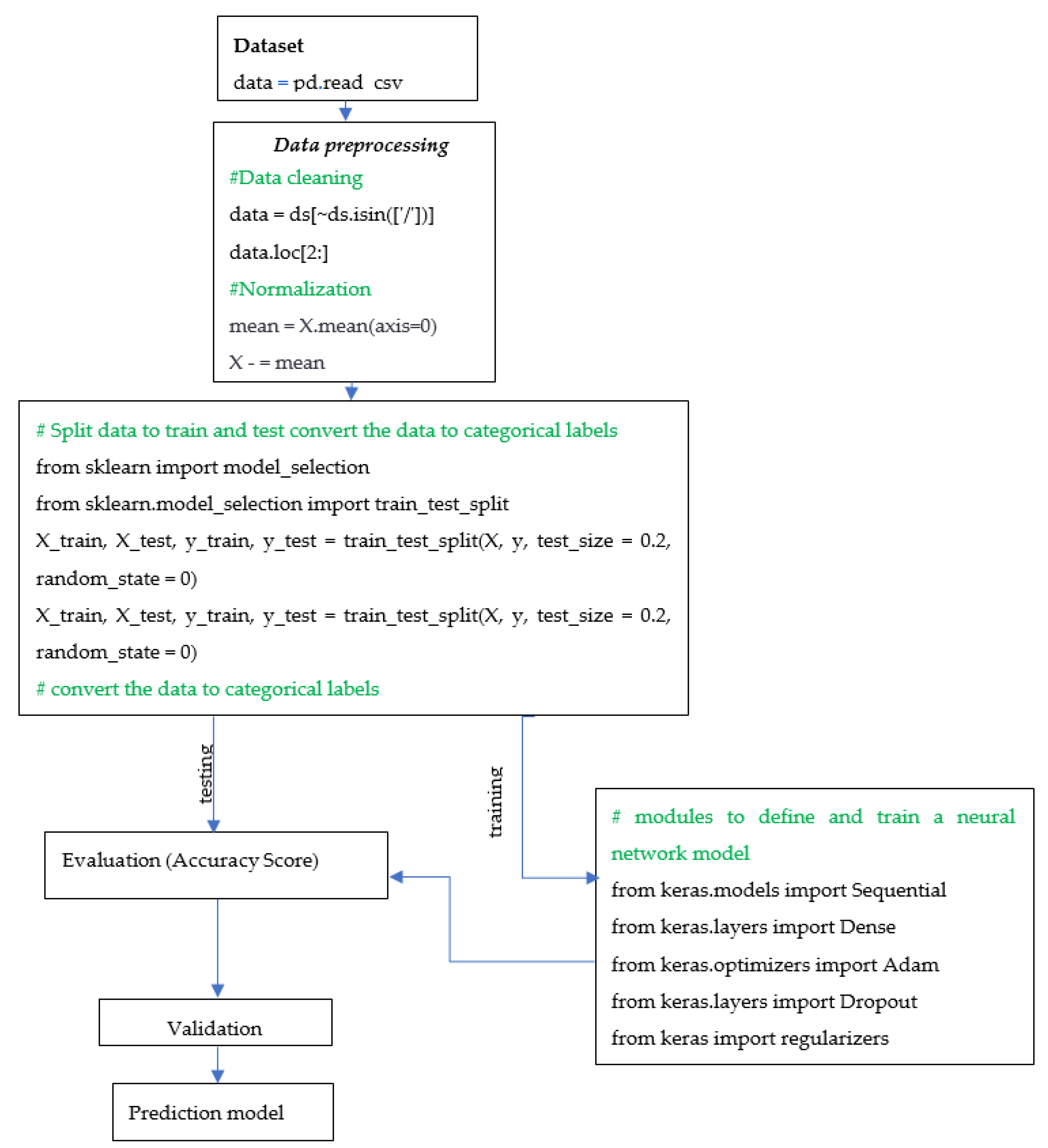
The algorithm is presented with a flowchart as Scheme 1, which shows the step-by-step process involved in constructing the neural network for prediction of obesity.

The implemented neural network model will be compared with the random forest model in terms of accuracy and predictions to evaluate their respective performance, considering that random forest is a popular algorithm suitable for small data. The random forest model is basically a large number of decision trees, which could be a couple of hundred, that would function in aggregate to improve the effectiveness of a prediction model. The scikit-learn library creates a random forest classifier and fits it to the training data.

3. Results and Discussion

Obese people’s problems start with “absence” or “minor” movement because the kinetics of their joints can threaten their stability due to insufficient quadriceps function [27,28]. Different models have been developed to investigate and monitor their health data [29] because being overweight and obesity are risk factors related with many diseases, a fact confirmed with the use of different modeling tools [30,31,32]. Research has confirmed [30] that a carefully planned and executed experiment in combination with appropriate mathematical models enables a better understanding of the complex endocrine regulation in obese people, and the aforementioned points to the exceptional potential of modeling applications.

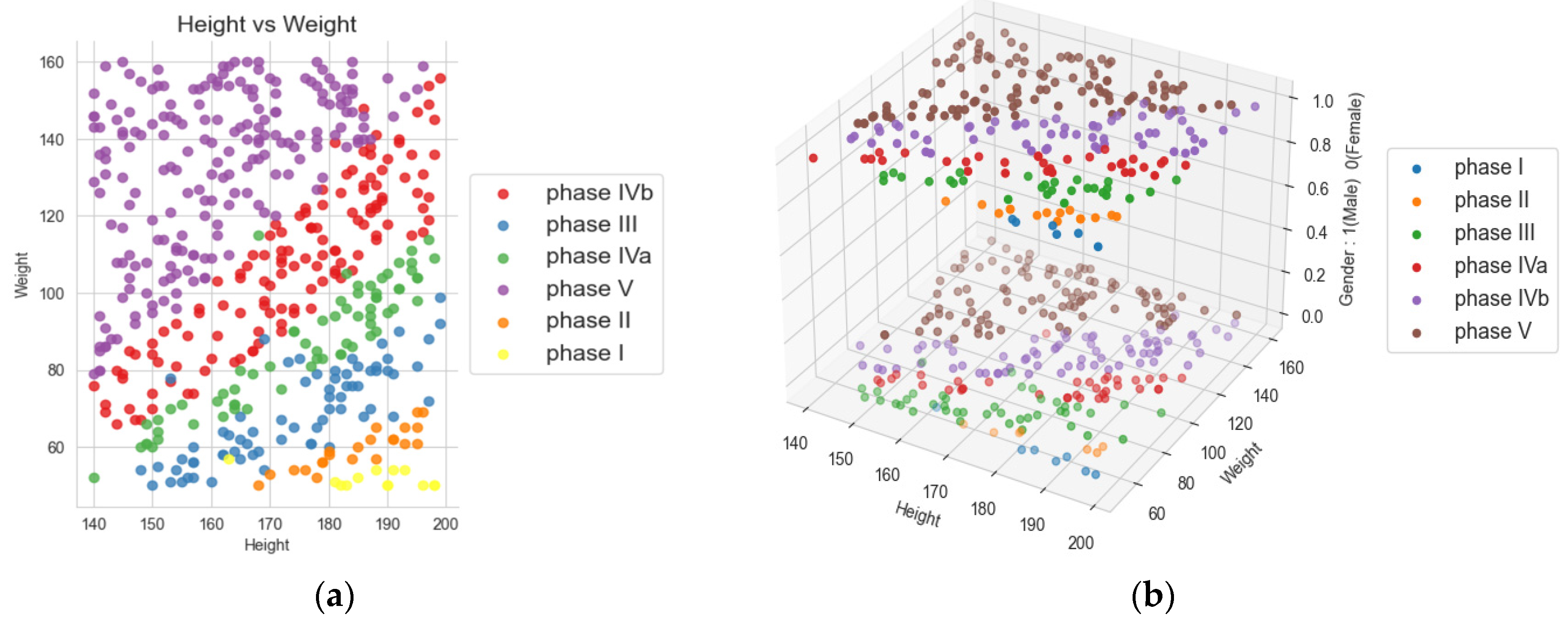
Therefore, this investigation should be a contribution to applying modeling tools in perception and identifying the changes in overweight and obese people in the weight loss program by applying the principles of the ketogenic diet. The data collected from the participants can be valuable for tracking their advancement throughout various stages of the ketogenic diet [2]. Figure 1 presents a scatter plot showing different phases for all the points in the data. Our objective is to train a model with higher accuracy and better health status by utilizing the data collected for BMI and other health parameters during the diet and observing their changes with the reduction in BMI and improvement in health parameters.

Above is a visualization as 2D and 3D charts utilized to track the progress of participants’ body mass index (BMI) during various phases of the ketogenic diet. These phases differ in terms of energy content, ranging from 800 to 1500 kcal, as well as nutrient composition [2]. The BMI serves as an initial indicator of excess body mass index above 25 [1], and a BMI over 30 kg/m² indicates obesity [31]. In other references, whereby the existence of certain groups/subgroups in the observed dataset will be evident [33], regardless of the age group starting from childhood [34], over adulthood [35], to the elderly [1,36], visualizations of the distribution and changes were observed. In this paper, in Figure 1, visualizations of the distribution and changes were observed through different phases of the ketogenic diet and in two groups, male and female.

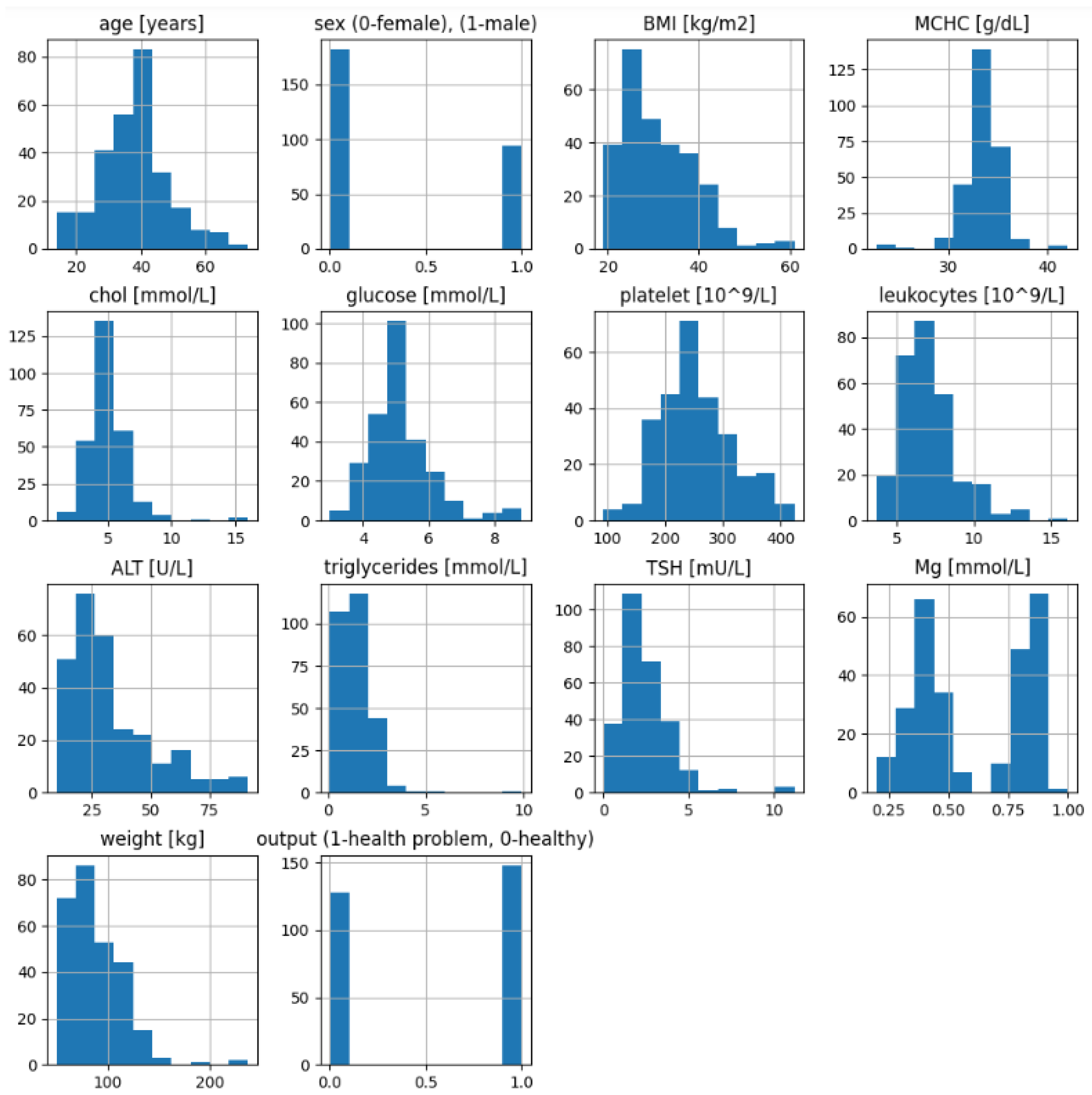
Additionally, Figure 2 shows the data distribution (plot histograms) of the health attributes of the participants at the beginning (before ketogenic diet) and their outcome of having any health problem (1)—whether diabetes, coronary disease, or another problem—or outcome (0) after diet with their reached weight (BMI).

Heatmaps are used to visualize the relationship between each attribute and the target variable [37]. A correlation matrix is used to visualize the correlations between all pairs of attributes in the dataset. This can help in determining which attributes are most strongly associated with the target variable if there is a linear correlation between them. In the heatmap Figure 3, a negative correlation (−0.9) can be seen between the attribute Mg and the target variable ‘output’, or (−0.6) between Mg and BMI, suggesting that higher Mg values are associated with lower BMI. Also in the Figure 3, are find the positive correlation (0.5) between glucose and cholesterol and ALT and sex suggests that there is some relationship between the levels of glucose and cholesterol and ALT and the sex of the individuals in the dataset. In [10], it was detected that ALT is correlated only with the female sex. All other pairs of attributes indicated a weak positive correlation. However, most of them have a non-linear correlation, for example, in studies of the Alzheimer’s disease pattern [38]. In fact, this is the idea of applying artificial intelligence and supervised learning, where its important inputs (features of participants) are paired with the corresponding target outputs. AI learns to map inputs to outputs during the training process [39].

Following the steps of algorithm of Scheme 1 in the process of constructing the neural network for the prediction of obesity, data collection follows the first step; then, preprocessing, where the data are cleaned, normalized and descriptive statistics are presented; in the next step, the dataset is split into training and testing using the ‘train_test_split()’ function from the ‘sklearn.model_selection’ module. The function takes several arguments, including the input features (x) and output variable (y), as well as the test size (in this case, 20% of the data is used for testing) and a random state value to ensure reproducibility. The purpose of converting the output variable to categorical labels is to prepare the data for use in a neural network that requires categorical labels as the output variable. The ‘to_categorical()’ function from the keras.utils.np_utils module is used to convert the output variables y_train and y_test into categorical labels.

The model architecture is then chosen. A common architecture for obesity prediction is a feedforward neural network with multiple hidden layers. The model is then trained using the training set; during training, the weights and biases of the neural network are adjusted to minimize the error between the predicted outputs and the actual outputs.

The model summary is shown in Figure 4 with the architecture of the neural network created using Keras. The model is sequential, meaning that the layers of the network are stacked sequentially. Figure 5 presents the model in detail.

The first layer is a fully connected layer with 16 neurons, which takes an input of 13 dimensions; the weights of this layer are initialized using a normal distribution. An L2 regularization with a value of 0.001 is added to the kernel to prevent overfitting. The activation function used in this layer is the rectified linear unit (ReLU). The second and third layers are dropout layers, which are added to prevent overfitting [39,40]. The dropout rate is set at 0.25. Dropout is used during the training phase; it involves randomly dropping units (neurons) with a specified probability (p) during each training iteration [41]. The fourth layer comprises eight neurons and is a fully connected layer. The fifth and final layer is also a fully connected layer with two neurons. The activation function used in this layer is softmax. The model is compiled using the RMSprop optimizer with a categorical cross-entropy loss function and accuracy as the evaluation metric. The learning rate for the optimizer is set at 0.001. Finally, the function returns the compiled model. The model summary is then printed using the summary() method, which provides a summary of the model architecture, including the number of parameters in each layer. “Param #” (short for parameter) represents the total number of trainable parameters in a neural network and includes all the weights and biases of the network. Each weight and bias contributes to the overall count of parameters. In the provided example, the total number of trainable parameters (Param #) is 378, which includes the weights and biases of the network. The individual layers and their corresponding Param # values are shown in Figure 5.

After training the neural network model [42,43], the model is evaluated using the testing set. Various performance metrics such as accuracy, precision, recall, and F1-score are commonly used. To prevent overfitting, weight regularization techniques are applied by adding a penalty term to the loss function that encourages the model to have smaller weights and reduces its overall complexity. 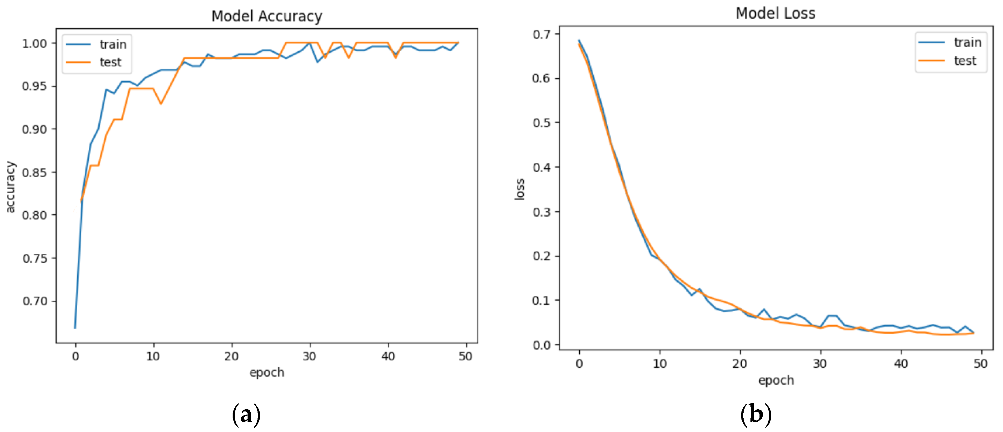Such an approach was also used in a prior study, where the theory of deep learning was applied for the screening of diabetic retinopathy (detection of bleeding) [44]. Trends of accuracy and model loss are presented in Figure 6. The plot of “Model Accuracy” presents the model’s performance. The legend shows which line represents which set of data, with “train” for training accuracy and “test” for validation accuracy.

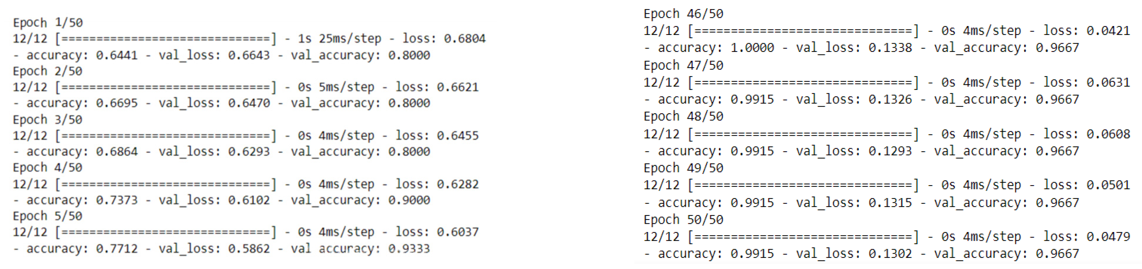
An epoch in the context of neural networks refers to a single iteration of the entire dataset through the neural network during the training process. During an epoch, the training algorithm updates the weights and biases of the neural network based on the error calculated for the output of the model. The number of epochs is a hyperparameter that can be tuned to improve the performance of the model. Increasing the number of epochs can help the model learn more from the data and potentially improve its accuracy but can also increase the overfitting risk. The model is trained for 50 epochs (complete passes through the training data).

The plot of “Model Loss” shows how the loss decreases over time during the training process. The training loss (blue line) and testing loss (orange line) should both decrease during training.

Each epoch shows the loss and accuracy on the training data (the data used to update the model’s parameters) and the validation data (a portion of the data held out during training to evaluate the model’s performance on unseen data). In this example, we see that as the number of epochs increases, the loss (a measure of how well the model’s predictions match the actual values) decreases and the accuracy (a measure of how many predictions the model got right) increases for both the training and validation data.

The model was trained for 50 epochs with a decreasing learning rate schedule. The training accuracy started at around 0.69 and increased to 1.0 by the end of the training. Similarly, the validation accuracy started at 0.63 and also increased to 0.98 by the end of the training. On the other hand, the training loss decreased from around 0.60 to 0.04 while the validation loss decreased from around 0.62 to 0.13. Both the training and validation loss decreased gradually throughout the training process. To improve results and simplify the problem, the binary classification of data is used [44]. Results are given in Figure 7.

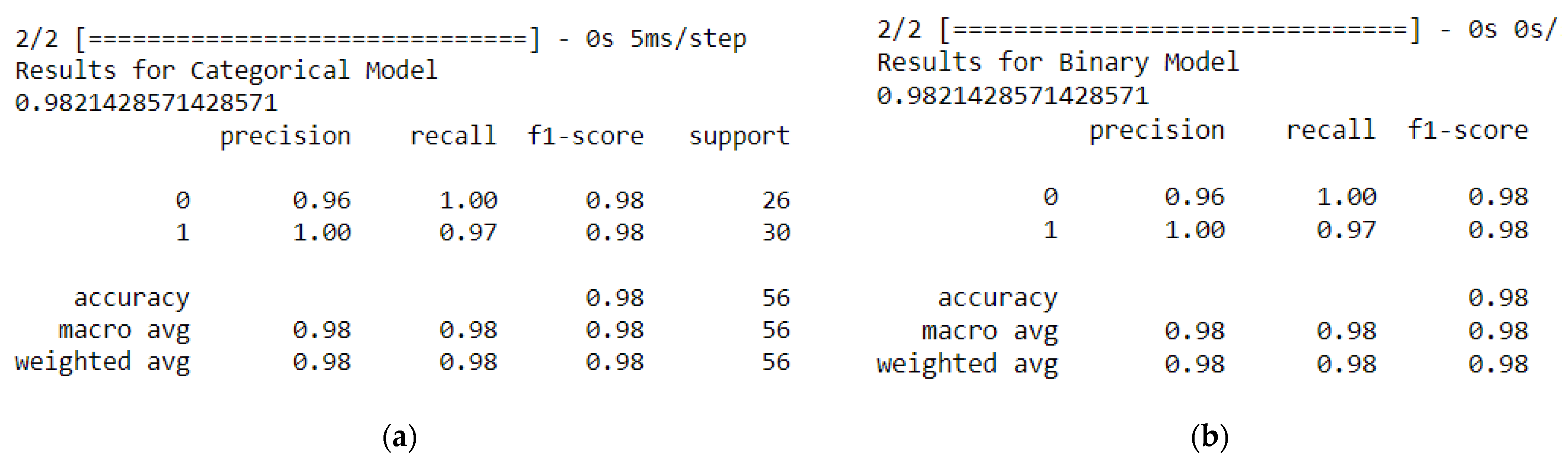
The validation accuracy is still high, indicating that the model is generalizing well to new data. In Figure 8, we can see the results from the classification report for the categorical model and the binary model.

The classification_report() function is used to generate a report of precision, recall, and F1-score for each class, as well as the average values for these metrics.

A high precision score of 0.96 means that the model is making fewer false positive predictions, while a high recall score of 1.0 means that the model is making fewer false negative predictions. A high F1-score of 0.98 indicates a good balance between precision and recall. As we can see in Figure 7, we have the same score results of the classification report for the categorical model and the binary model.

In the context of the health problem prediction and BMI, precision, recall, and F1-score are used to evaluate how well the models are performing at identifying patients with and without health problems.

The accuracy_score() function from scikit-learn is used to calculate the accuracy score of 0.98 of the categorical model on the test dataset, which is the percentage of correctly classified samples, which means 98% of the samples in the test dataset were correctly classified by the model. Such accuracy is common even when neuro-fuzzy classifiers are used [45,46].

The macro average and weighted average for precision, recall, and F1-score are also reported. The macro average calculates the average performance across all classes, while the weighted average considers the number of samples in each class. Overall, the model has a high level of performance, with precision 0.96, macro and weighted averages 0.98, recall 0.98, and F1-score above 0.98.

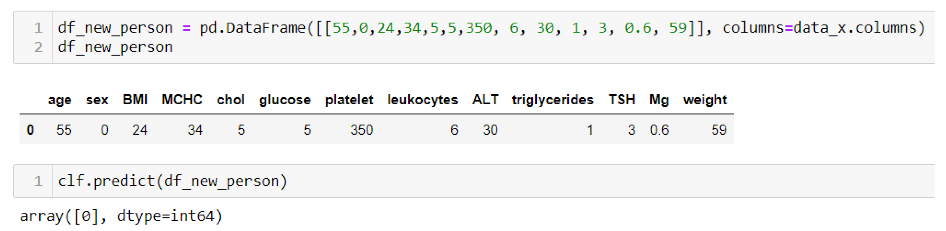
The next step in the context of health problem prediction and BMI is to perform prediction tests of some individual person with specific health parameters and their own BMI. Several tests were conducted with normal and elevated levels of glucose in the blood along with cholesterol parameters (Figure 9).

An output of 1 is obtained in the case when some of the parameters have an increased value—for example, glucose, cholesterol, triglycerides, or platelets—but also BMI (Figure 8), where an output of 0 (Figure 10) is obtained if the parameters are within the normal range and BMI.

In the final step, the dataset of participants was also evaluated with random forest models, considering that random forest is a popular algorithm suitable for small data. Importing the RandomForestClassifier class from ‘sklearn.ensemble‘ implements the random forest algorithm for classification tasks and assigns it to the variable ‘clf_rf’. Fitting the classifier to the training data, clf_rf.fit(x_train, y_train), the ‘clf_rf’ object will be a trained random forest classifier that can be used for making predictions on new data. The scikit-learn library is used to calculate the accuracy scores for the trained random forest classifier on both the training and test data. The accuracy_score(y_test, clf_rf.predict(x_test)) = 0. 0.96 means that the model correctly predicted the target variable for 96% of the samples in the test data, and accuracy_score (y_train, clf_rf.predict(x_train)) = 0.99 means that the model correctly predicted the target variable for 99% of the samples in the training data.

The prediction was also conducted with random forest models, and we obtained the same prediction (Figure 9 and Figure 10).

In the context of a health problem prediction project, the accuracy_score function is used to evaluate the performance of neural networks comprising random forest. The results revealed that both models performed very well with high accuracy scores. The accuracy_score for random forest on the test dataset was 0.96, indicating its ability to predict health problems with a high level of accuracy. It was expected that the random forest model would show high performance because of small data. The neural networks model also achieved a high accuracy score of 0.97, demonstrating high performance in predicting health problems. These results suggest that both models can effectively predict health problems; however, the neural networks model outperformed in terms of accuracy compared with other research references and considering the complexity of overfitting.

This is certainly a significant improvement over logistic regression classifiers, which range between 0.903 and 0.917 in the prediction of comorbidity (more than one chronic disease), investigated by Lu and Uddin [47].

Comparative analysis of the results is essential to evaluate the effectiveness of our proposed obesity prediction system. Studies directly related to our work are limited in number. We identified some relevant studies in the areas of childhood obesity risk prediction, diabetic risk prediction from obesity, and disease prediction. Despite the scarcity of comparable studies, we made efforts to compare our work with others based on specific parameters. Feng et al. [48] used random forest to recognize 19 types of physical activities with 93.4% accuracy, although the limited number of subjects may impact generalizability. Kanerva et al. [49] employed random forest to explore factors affecting body weight, reporting an estimated error rate of 40% and highlighting the algorithm’s ability to handle highly correlated variables; however, the accuracy of the model was affected by the low number of correlated variables used in the study. In the study of Ferdowsy et al. [50], if we compare the results regarding accuracy—k-NN, 77.5%; random forest, 72.3%; and logistic regression, 97,09%—we can see that the accuracy of our developed neural network model is very close to the accuracy of logistic regression, which represents a significant advance in nutrition and neural network applications. It must be emphasized that this high accuracy was achieved due to the nature of the data. The dataset has 400 points. All 200 patients who were overweight and had some health problem, under the keto diet regime, had rich biochemical results regulated as well as their weight. The data training was in 50 iterations; so, a very well-trained model was achieved.

4. Conclusions

With the application of artificial intelligence in the field of nutrition, such as neural networks and random forest models, it is possible to identify the factors that influence obesity and predict an individual’s weight loss progress. These models can help guide healthcare professionals in developing personalized nutrition plans and making recommendations for adjustments to an individual’s energy intake.

The accuracy of these models is important to ensure that individuals are receiving appropriate recommendations for their unique circumstances. Creating machine learning models to forecast weight loss and health outcomes has the potential to revolutionize the field of nutrition and help individuals achieve their weight loss goals in a safe and effective manner. It should be noted that these models should be used in conjunction with guidance from healthcare professionals to ensure that individuals are receiving the best possible care.