Real-Time Deployment of MobileNetV3 Model in Edge Computing Devices Using RGB Color Images for Varietal Classification of Chickpea

Abstract

Chickpeas are one of the most widely consumed pulses globally because of their high protein content. The morphological features of chickpea seeds, such as colour and texture, are observable and play a major role in classifying different chickpea varieties. This process is often carried out by human experts, and is time-consuming, inaccurate, and expensive. The objective of the study was to design an automated chickpea classifier using an RGB-colour-image-based model for considering the morphological features of chickpea seed. As part of the data acquisition process, five hundred and fifty images were collected per variety for four varieties of chickpea (CDC-Alma, CDC-Consul, CDC-Cory, and CDC-Orion) using an industrial RGB camera and a mobile phone camera. Three CNN-based models such as NasNet-A (mobile), MobileNetV3 (small), and EfficientNetB0 were evaluated using a transfer-learning-based approach. The classification accuracy was 97%, 99%, and 98% for NasNet-A (mobile), MobileNetV3 (small), and EfficientNetB0 models, respectively. The MobileNetV3 model was used for further deployment on an Android mobile and Raspberry Pi 4 devices based on its higher accuracy and light-weight architecture. The classification accuracy for the four chickpea varieties was 100% while the MobileNetV3 model was deployed on both Android mobile and Raspberry Pi 4 platforms.

1. Introduction

Pulses constitute one of the most significant crops in the leguminous family. About 90 million metric tonnes of pulses are produced worldwide [1]. Common beans, lentils, chickpeas, dry peas, cowpeas, mung beans, urad beans, and pigeon peas are the main pulses farmed worldwide. Pulses are significant sources of protein, phosphorus, iron, calcium, and other essential minerals, and help millions of individuals in impoverished nations meet their nutritional needs [2,3]. Pulses have recently acquired popularity on a global scale as an alternative to animal-based sources of protein [4]. With a production of 15 million metric tonnes and a third-place ranking among pulses after beans and peas, chickpeas are one of the high protein pulses grown in more than 57 nations [1]. Depending on the cultivar, agronomic practices, and climatic factors, the protein content of chickpeas varies from 17% to 24% [5]. Additionally, chickpeas are a good source of energy and include vitamins, minerals, fibre, and phytochemicals. According to Wood and Grusak, 2007 [6], regular consumption of chickpeas lowers the risk factors for diabetes, cancer, and cardiovascular disease.

For processors, customers, and other stakeholders, the quality of chickpeas is crucial in influencing their preference [7]. The various factors considered in evaluating the quality of chickpeas are 100-seed weight, ash content, colour, cooking time, cooked chickpea seed stiffness, moisture content, protein content, seed size distribution, starch content, total dietary fibre, water absorption, and others [8]. It is difficult to assess the quality of a sample that contains mixed chickpea varieties, so maintaining varietal purity is the first crucial step in determining chickpea quality. Prior to a deeper examination of their visible or internal properties, the identification or classification of chickpea types assumes relevance. The most used imaging method for classifying agricultural products by varietal is RGB imaging [9]. Around the world, different chickpea cultivars are produced in various agroclimatic zones. The nutrient content, physical characteristics, and economic worth of each variety vary. Different chickpea varieties can be identified by their physical characteristics, such as colour and texture, which are visible and aid in classification. However, this classification process is time-consuming, expensive, and frequently performed by human professionals. Due to the intricacy of the task and the abundance of visual and environmental components, research into the creation of tools for the automation of these occupations is still underway. The need for accurate variety identification systems in precision agriculture is also growing as a result of the ramifications for the economy, ecology, and society [10].

Deep learning models are being used more frequently, which has led to significant improvements, notably in classification tasks [11,12,13,14,15]. Deep learning has been used in recent research for agricultural crop classification due to the increased accuracy and hardware accessibility. In addition, the rapid advancement of open-source hardware in recent years has promoted the creation and use of low-cost agricultural surveillance tools with image processing and AI capabilities. Single-board computers (SBCs) in many configurations, like the Raspberry Pi (RPi), have spread quickly across many different applications like food manufacturing [16] and surveillance monitoring [17]. Osroosh et al., 2017 [16] detailed the design and construction of a monitoring system that employs thermal and RGB images, built on a Raspberry Pi 3, that is able to operate in difficult real-world scenarios. Raspberry Pi was utilised by Hsu et al., 2018 [18] to build a low-cost monitoring network for agricultural applications that is intended for wide adoption. A monitoring environment with many devices and interfaces was developed by Morais et al., 2019 [19], enabling communication in low-cost agricultural equipment.

In light of this backdrop, the current work provides the results of training using transfer learning in architectures that have just been investigated for agricultural applications, as well as their implementation on affordable hardware like the android mobile and Raspberry Pi 4 microcomputer. In order to obtain findings that help in the classification of chickpeas, one of the objectives of this research is to incorporate CNN models in a low-cost, low-power device that can process information in real time. Therefore, four common Canadian chickpea varieties were utilised and an attempt was made to identify them utilising computer vision and machine-learning-based methodologies in order to automate the process of chickpea classification. The work’s goal is broken down into two subcategories. The first stage involves creating the classification model using computer vision and machine-learning-based approaches. The deployment phase, which involves deploying the trained machine-learning model on Android mobile and Raspberry Pi 4 devices, and evaluating its performance, takes place in the second stage.

2. Materials and Methods

In this study, the Crop Development Centre (CDC), University of Saskatchewan, Saskatoon, Canada, provided four popular Canadian chickpea varieties (CDC-Alma, CDC-Consul, CDC-Cory, and CDC-Orion) harvested in 2020. To remove unwanted foreign particles, the seeds were sieved. The seeds were also hand-sorted to remove broken, mouldy, and discoloured seeds, as well as washed to remove any leftover dust particles. The initial moisture content of each variety of cleaned chickpeas was evaluated after 24 h in a 105 °C hot air oven [20]. To achieve equal moisture distribution among the samples, all chickpea varieties were reconditioned to 12.5 ± 0.5% wet basis by adding measured distilled water and well mixing it, followed by seven days of storage in airtight low-density polyethylene (LDPE) bags at 5 °C.

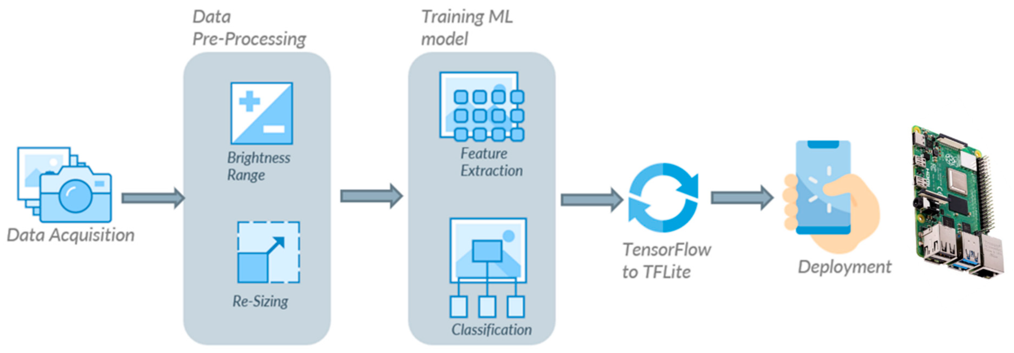
The proposed approach in this study is presented as a block diagram in Figure 1. It combines data acquisition, pre-processing, model training, and deployment. The images used for the experiment were collected using a smartphone camera and an industrial camera in a natural lightning environment. Various data pre-processing techniques were used to augment the existing dataset. For training purposes, transfer learning was used to create and train machine-learning models. The model evaluation was performed on a separate test dataset. Thereafter, the optimal machine-learning model was deployed on an Android device and a Raspberry Pi 4 to check its real-time performance.

2.1. Data Acquisition

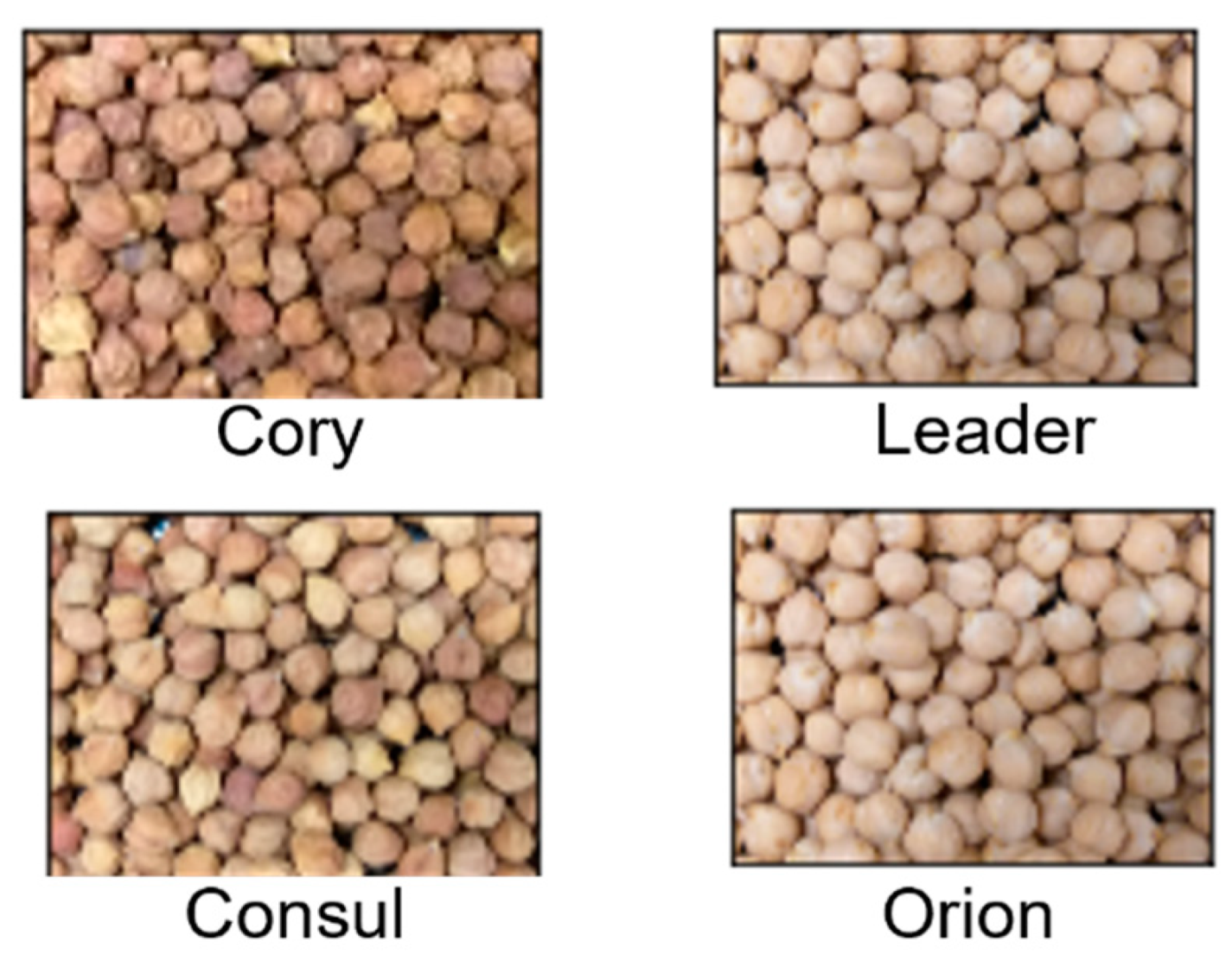
To build robust classification models, the RGB images of the chickpea sampled were captured using two different cameras (smartphone camera and industrial camera) to accommodate potential variations due to imaging systems. The smartphone (Samsung Galaxy A6 Plus) used comes with a dual camera, where the primary camera has 16 MP, followed by 5 MP for the secondary camera with an f/1.7 aperture opening. First, the chickpeas were placed in a tray in a manner such that it was fully filled with chickpeas. In order to collect images through a smartphone, the smartphone camera was set on top of the chickpea tray in such a way that it could capture the maximum area of the tray without including the borders of the tray. The images were 3456 × 4608 in resolution and a total of 150 images were collected for each variety. As for the industrial camera, a GigE colour industrial camera (Model: DFK 33GX273; Specifications: 1.6 MP, 60 FPS; The Imaging Source, USA) was used. The chickpea seeds were placed over a conveyor belt and the speed of the belt was fixed at 1 m/min to avoid image distortion. The industrial camera was set up on top of a conveyor belt and the video of the chickpea variety was captured. Thereafter, the video was processed and each frame of the video was extracted as an image. The extracted images were used to build our chickpea dataset with different cameras. Thereafter, a total of 400 images were collected for each variety from captured video with 1440 × 1080 resolution. Thereafter, all the images were combined (smartphone and industrial camera) and the final dataset consisted of 550 images per variety. The reason behind using two different sources of dataset (i.e., industrial camera and smartphone) is to increase the variability in the dataset which helps in better generalisation by the model. In other words, it will increase the robustness of our trained model since each source of data is exposed to different environmental conditions and, by combining the data, the model becomes more tolerant to changes in lighting, noise, and other factors, producing more reliable and accurate results. Further, this variability will make the model better generalise on datasets acquired with different camera resolution and conditions. Figure 2 displays the collected images for the four chickpea varieties.

2.2. Data Augmentation

Image data augmentation is a way of artificially increasing the amount and diversity of a training dataset by realistically transforming images currently in the training dataset. Data augmentation aids in the building of more efficient models, which improves the model’s generalisability, and prevents overfitting and the problem of the network memorising specific information of the training images [21,22]. Image alteration methods used in this work for real-time augmentation include rotation, horizontal and vertical translation, shear, and zoom. The training dataset is made up of both the original images and the augmented images produced through alterations.

Different pre-processing techniques were applied using the ImageDataGenerator function defined in TensorFlow.

Table 1. Different data augmentation parameters along with their values.

Parameter	Value
Rotation Range	40
Horizontal Flip	True
Width Shift Range	0.2
Height Shift Range	0.2
Shear Range	0.2
Zoom Range	0.2

shows the list of different data augmentation pre-processing techniques and their values. The rotation range rotates the image clockwise by a given number of degrees. A horizontal flip flips the image horizontally. The width shift range shifts the image left or right by considering the given number as a percentage (i.e., 0.2 = 20%). The height shift range shifts the image up or down by considering the given number as a percentage. Shear range distorts the image by considering the given value as an angle. Zoom range zooms the image by considering the given number as a percentage.

2.3. Feature Extraction

The present work uses a CNN-based model for extracting features from the input images. In our study, three different models named NasNet-Mobile, MobleNetV3-Small, and EfficientNetB0 were selected. The architecture of these models is fast and efficient, designed for frequent or real-time predictions on mobile devices and single-board computers [23,24]. All three models are designed using neural architecture search (NAS) to achieve optimal architecture for on-device machine learning. NAS is the process of automatically searching for the optimal deep neural network (DNN) architecture using three major components: search space, optimisation methods, and candidate evolution methods. The main idea of search space is to define the optimal architecture of the model by considering the input dataset [25]. Since it requires prior knowledge of the dataset, it is not ideal for novel domains. Another problem with search space is its limitations in exploring the available architecture, as some of the excluded architecture might be a better choice. Optimisation methods help search space determine the best possible architecture by considering the effectiveness of the selected architecture. The last component, candidate evolution, is designed for comparing the results produced by optimisation methods and helps search space choose the best possible architecture [26].

2.3.1. NasNet-A (Mobile)

The first model used in our study was NasNet-A (mobile). As the name suggests, the architecture of this model was developed using NAS. Researchers redesigned a search space (the first component of NAS) by including controller recurrent neural network (RNN) in order to obtain the best architecture for the CIFRA 10 dataset. Thereafter, the same architecture (NasNet architecture) was taken, and stacking of the copies of the developed CNN layers on each other was performed and applied to the ImageNet dataset. As a result, the new architecture was able to achieve 82.7% top-1 and 96.2% top-5 accuracy on the ImageNet dataset.

Table 2. NasNet-A (mobile) model architecture.

Stage	Operator	Resolution	Channels	Layers
1	Conv2D, 3 × 3	224 × 224	3	1
2	Reduction Cell	111 × 111	32	2
3	Normal Cell	28 × 28	44	4
4	Reduction Cell	28 × 28	88	1
5	Normal Cell	14 × 14	88	4
6	Reduction Cell	14 × 14	176	1
7	Normal Cell	7 × 7	176	4

showcases the high-level representation of the used NasNet-A (mobile) architecture. As can be observed from the table, the architecture consists of reduction cells and normal cells. Reduction cells produce a feature map of their inputs by reducing their height and weight, whereas normal cells produce a feature map with the same dimensions as their inputs [27].

2.3.2. MobileNetV3 (Small)

The second model chosen was MobileNetV3 (small) because of its high efficiency for on-device machine learning. In order to develop the cell for MobileNetV3, researchers took MobileNetV2′s cell (consisting of residual and linear bottlenecks) and added squeeze-and-excite to the residual layers. Moreover, upgraded layers (with modified switch non-linearities), squeeze, and residual have sigmoid functions instead of sigmoid to get better results. After designing this cell, NAS was applied to obtain the best possible network architecture. Additionally, researchers also applied the NetAdapt algorithm to the developed model to fine-tune each layer. The model had 67.5% top-1 accuracy with 16.5 ms average latency on the ImageNet dataset.

Table 3. MobileNetV3 (small) model architecture.

Stage	Operator	Resolution	Channels	Layers
1	Conv2d, 3 × 3	224 × 224	3	2
2	Bottleneck, 3 × 3	112 × 112	16	2
3	Bottleneck, 3 × 3	56 × 56	16	2
4	Bottleneck, 3 × 3	28 × 28	24	1
5	Bottleneck, 3 × 3	28 × 28	24	2
6	Bottleneck, 3 × 3	14 × 14	40	1
7	Bottleneck, 3 × 3	14 × 14	40	1
8	Bottleneck, 3 × 3	14 × 14	40	1
9	Bottleneck, 3 × 3	14 × 14	48	1
10	Bottleneck, 3 × 3	14 × 14	48	2
11	Bottleneck, 3 × 3	7 × 7	96	1
12	Bottleneck, 3 × 3	7 × 7	96	1
13	Conv2d, 1 × 1	7 × 7	96	1
14	Pool	7 × 7	576	1
15	Conv2D, 1 × 1, NBH	1 × 1	576	1
16	Conv2D, 1 × 1, NBH	1 × 1	1024	1

indicates the high-level architecture of the model [28].

2.3.3. EfficientNetB0

The third model selected for the study was EfficientNetB0 because of its state-of-the-art accuracy, small size, and speed compared to other ConvNets. In order to develop the EfficientNet, researchers used NAS on a new mobile-sized convolutional network and came up with EfficieNetB0, which had 77.1% top-1 accuracy and 93.3% top-5 accuracy on the ImageNet dataset. In order to make EfficientNetB0 more efficient, researchers proposed a new compound scaling method that uniformly scales all dimensions (depth, width, and resolution) of any given model and used that method on EfficientNetB0 to produce better versions of it (i.e., EfficientNetB1, EfficientNetB2, EfficientNetB3, EfficientNetB4, EfficientNetB5, EfficientNetB6, and EfficientNetB7). For our study, we used EfficentNetB0, which consists of a mobile inverted bottleneck MBConv cell and squeeze-and-excitation, as shown in

Table 4. EfficientNetB0 architecture.

Stage	Operator	Resolution	Channels	Layers
1	Conv2d, 3 × 3	224 × 224	32	1
2	MBConv1, k 3 × 3	112 × 112	16	1
3	MBConv6, k 3 × 3	112 × 112	24	2
4	MBConv6, k 5 × 5	56 × 56	40	2
5	MBConv6, k 3 × 3	28 × 28	80	3
6	MBConv6, k 5 × 5	14 × 14	112	3
7	MBConv6, k 5 × 5	14 × 14	192	4
8	MBConv6, k 3 × 3	7 × 7	320	1
9	Conv2D, 1 × 1	7 × 7	1280	1

[29].

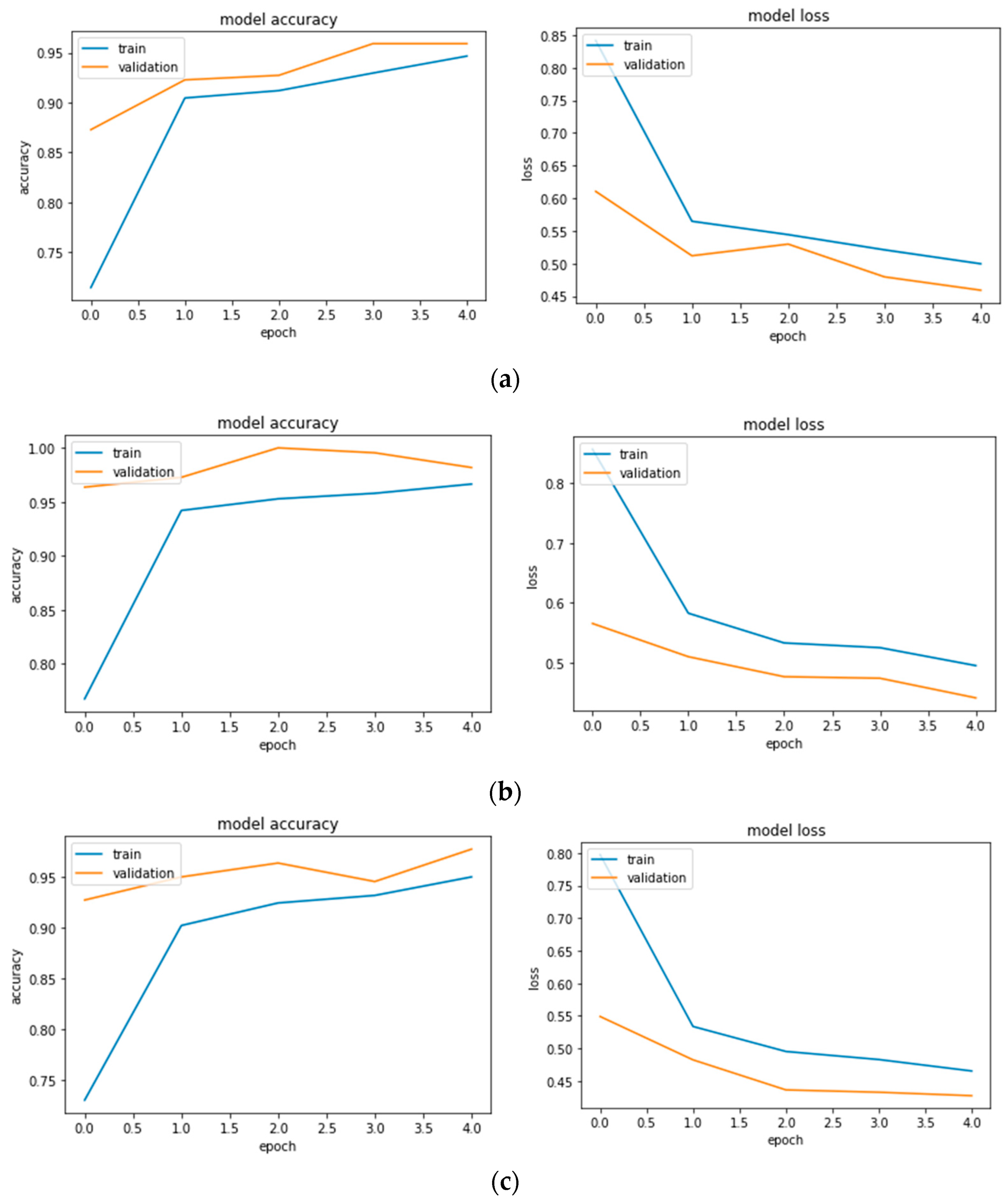
2.4. Training of CNN Architectures

The chickpea image dataset was organised into four labelled files, each with 550 original images. The dataset was split into three parts: training, validation, and testing. The training was performed on 80% of the original images, with the remaining 10% used for validation and the other 10% for testing. As a result, the 80:10:10 ratio was consistent across all varieties and models. The validation set was used to validate training performance, whereas the test set was used to validate classifier performance. The images for training, validation, and testing were chosen by initialising the GPU random seeds to ensure that the model networks were trained, validated, and tested on the same dataset. All three model architectures utilised in this work were trained five times using five different random seeds and the findings reported in this study are for a single random seed (3) shared by all model architectures. The different hyperparameters utilised during network training, such as momentum, number of epochs, and optimiser (stochastic gradient descent), were modified to properly train the CNN for image classification. Momentum is employed during network training to accelerate the learning rate. An epoch is the number of times the network traverses the complete training dataset. It is important to note that the number of epochs that a model should be trained for depends on a number of factors, including the size and complexity of the dataset, the complexity of the model, and the desired level of accuracy. The optimiser is used to update the network’s learnable parameters during training in order to reduce the loss function [30]. The settings of these hyperparameters (

Table 5. Values of hyperparameters used in machine-learning models.

Parameters	Values
Max Epochs	5
Mini Batch Size	32
Optimiser	Stochastic Gradient Descent (SGD)
Initial Learning Rate	0.005
Momentum	0.9
Loss Function	Categorical Cross Entropy

) were chosen based on available literature and then kept constant to allow for fair comparisons between networks [31]. The learning rate specifies how frequently the weights in the layers are updated during training, whereas the batch size specifies the number of images used to train the network in each epoch. The minimum and maximum ranges of the hyperparameters were determined through several trials and based on existing related literature. Since the training was performed on pre-trained networks with defined weights, the learning rate was kept low at 0.005. A very low learning rate may result in prolonged training time without convergence, while a very high learning rate may result in poor learning of complexity from the training dataset [32]. Similarly, choosing the right batch size is critical for network training because a small batch size will converge faster than a large batch size. Furthermore, a bigger batch size will achieve optimum minima, which a very tiny batch will find difficult to achieve. For the training, `TensorFlow Lite Model Maker` was used that simplified the process of training a TensorFlow Lite model using custom dataset. It uses transfer learning to reduce the quantity of required training data and training time, resulting in fewer epochs of model training. In this study, we have added two layers, a dropout layer and a dense layer, after each pre-trained CNN. The dropout rate used was 20% in the dropout layer and the dense layer had four units, or neurons, in order to classify four different varieties of chickpea with the SoftMax activation function. The study was conducted on a Google Colab configured with an NVIDIA Tesla K80 GPU and 12 GB of RAM.

2.5. Model Evaluation

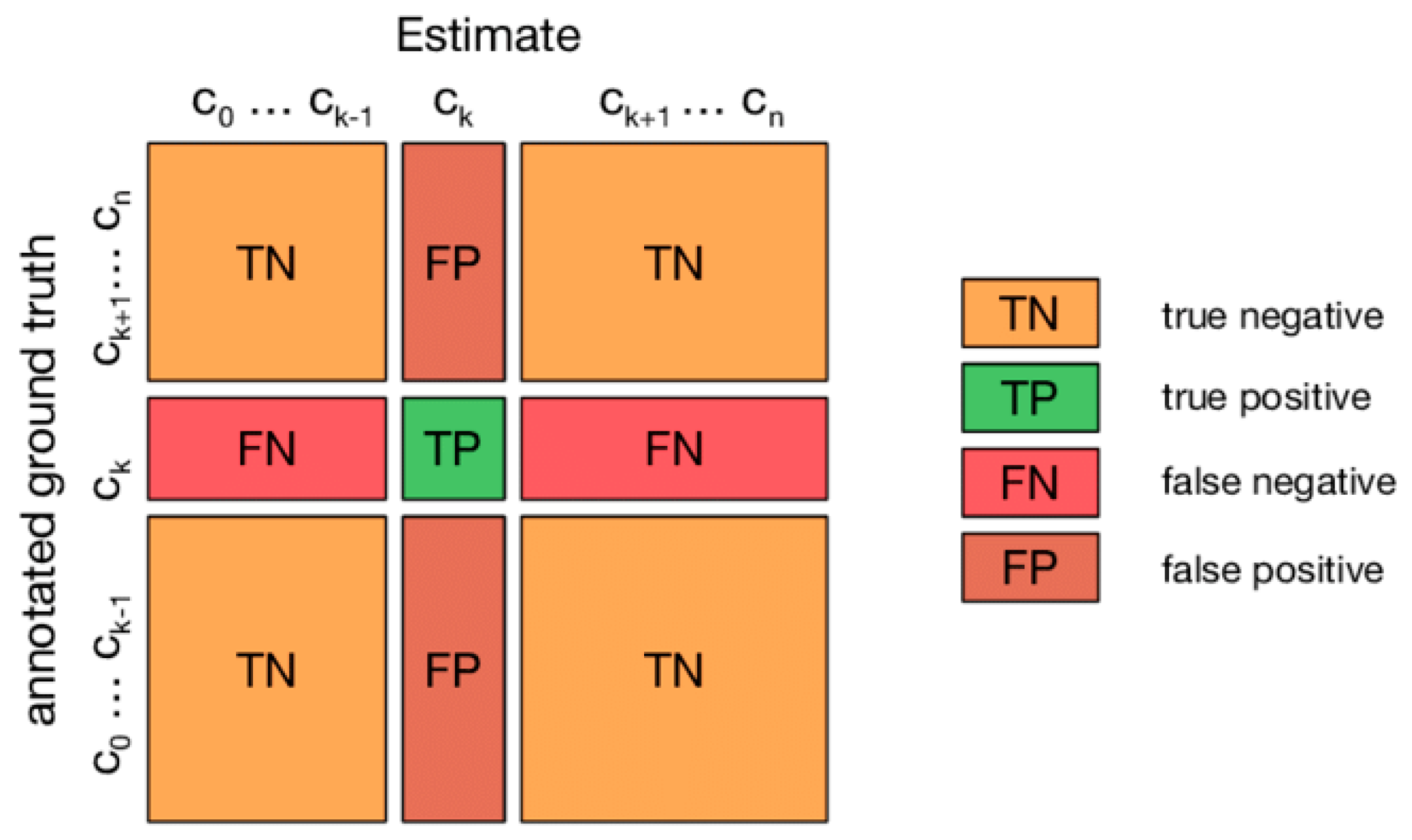
In this study, the model’s performance was assessed using accuracy, precision, sensitivity, and specificity obtained from the confusion matrix of the models [33].

$$\mathrm{Accuracy}=\frac{\mathrm{T}\mathrm{P}+\mathrm{T}\mathrm{N}}{\mathrm{T}\mathrm{P}+\mathrm{T}\mathrm{N}+\mathrm{F}\mathrm{P}+\mathrm{F}\mathrm{N}}$$

(1)

$$\mathrm{Precision}=\frac{\mathrm{T}\mathrm{P}}{\mathrm{T}\mathrm{P}+\mathrm{F}\mathrm{P}}$$

(2)

$$\mathrm{Specificity}=\frac{\mathrm{T}\mathrm{N}}{\mathrm{T}\mathrm{N}+\mathrm{F}\mathrm{P}}$$

(3)

$$\mathrm{Sensitivity}=\frac{\mathrm{T}\mathrm{P}}{\mathrm{T}\mathrm{P}+\mathrm{F}\mathrm{N}}$$

(4)

where TP, TN, FP, and FN represent true positive, true negative, false positive, and false negative, respectively. True positive is a consequence in which the model predicts the positive class accurately and true negative indicates accurate prediction of the negative class. False positive indicates the incorrect prediction of the positive class by the model and false negative indicates the incorrect prediction of the negative class.

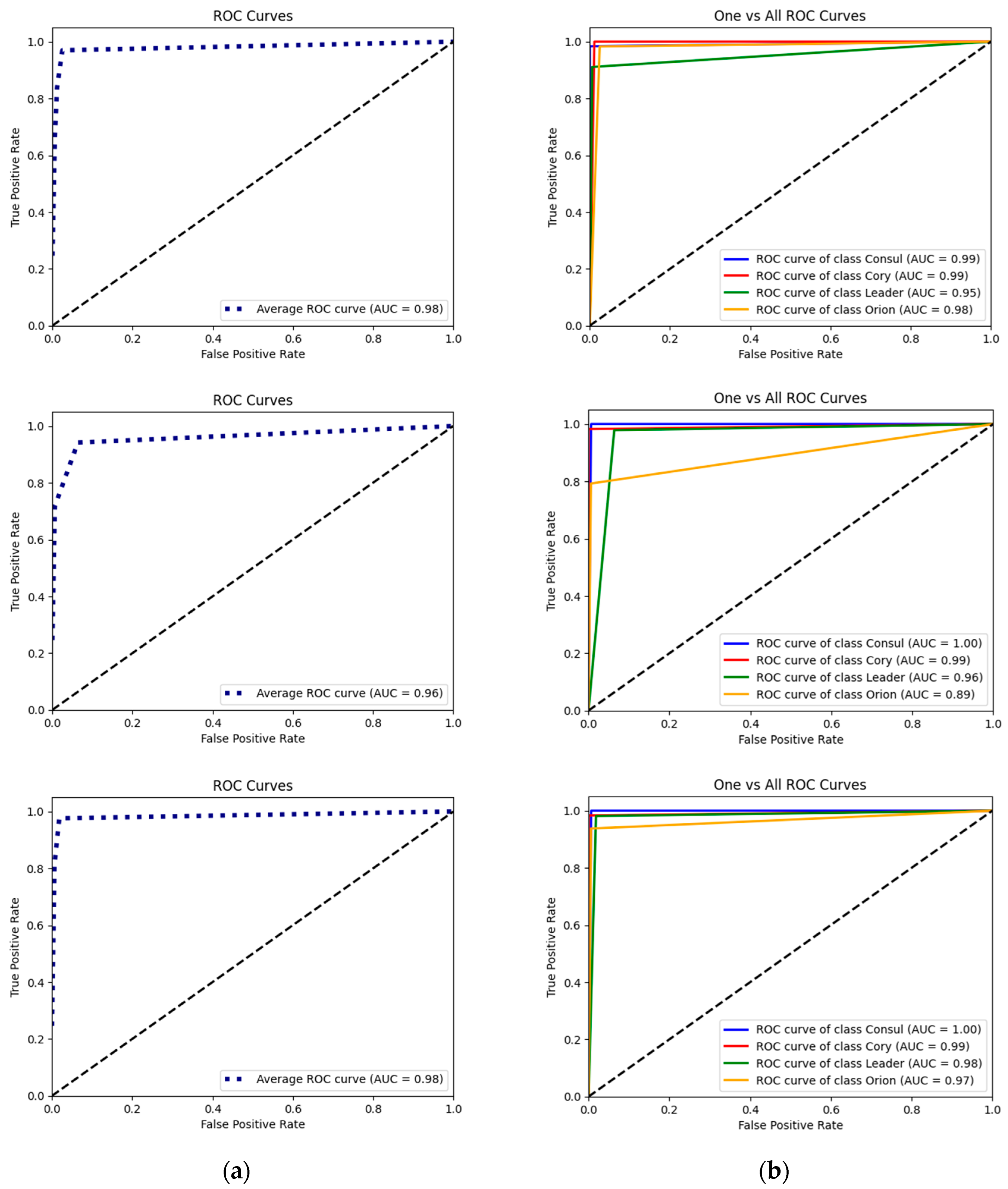
In addition to the previously mentioned metrics used to evaluate classifier performance, the models were also assessed based on the area under the receiver operating characteristic (ROC) curve, known as AUC. AUC is a significant scalar value that provides an overall assessment of a classifier’s performance. The ROC curve plots the true positive rate (TPR) against the false positive rate (FPR), with TPR on the y-axis and FPR on the x-axis. AUC measures the classifier’s ability to distinguish between classes and represents the degree of separability. It ranges from 0.5 to 1.0, where the minimum value corresponds to a random classifier and the maximum value indicates a perfect classifier. AUC has the advantageous properties of threshold and scale invariance, making it a robust metric. This implies that AUC is not influenced by the chosen threshold or the scale of probabilities. Computationally, AUC is determined by aggregating trapezoid areas beneath the ROC curve. AUC values between 0.7 and 0.8 are considered acceptable, 0.8 to 0.9 as excellent, and greater than 0.9 as outstanding [33].

The classification time measure would utilise the model’s average time to predict an image class. This was accomplished by employing a timer at the beginning and end of the evaluation procedure, and the classification time was calculated using the following formula [34]:

$$\mathrm{Classification} \mathrm{time}=\frac{Test evaluation time}{Number of steps\times Batch size}$$

(5)

The Python batch dataset format was applied to the test dataset. The batch size hyperparameter was used to group the images in this format. A batch in this experiment consisted of 32 images.

2.6. Confusion Matrix

The confusion matrix of the test set was used to assess the models’ performances. The confusion matrix results give the quantitative and predictive values for chickpea varietal categorisation. The anticipated class/output class is on the X-axis of the matrix shown in Figure 3, while the true class/target class is on the Y-axis. The diagonal cells in the matrix reflect correctly categorised observations, showing that the anticipated and actual classes are the same, whereas the remaining observations have been misclassified [33].

2.7. Deployment Platforms

Among the three studied machine-learning models, it is planned to deploy the model with optimal performance on an Android device and a Raspberry Pi 4 device to verify its functionality in the real world.

2.7.1. Mobile Application Development

To deploy trained machine learning on mobile devices, the models were converted to TensorFlow Lite termed interpreters in the format of “.tflite” files using the TensorFlow Lite Task Library API. TensorFlow Lite is a collection of tools built for edge, embedded, and mobile devices, allowing for on-device machine learning. The benefits of edge machine learning include real-time latency (no data offloading), privacy, robustness, connectivity, a smaller model size, and efficiency (costs of computation and energy in watts per FPS). It supports Linux, Android, iOS, and the MCU. The TensorFlow Lite converter and TensorFlow Lite interpreter are two components for the deployment of TensorFlow models on mobile devices [35]. To begin, the Keras model that is created using the TensorFlow 2.0 library was exported to pb (protocol buffer) models. Second, the PB models were converted to TensorFlow Lite models using the TensorFlow Lite Converter. 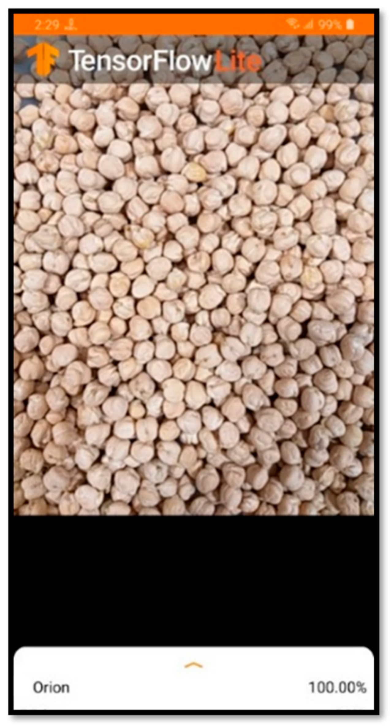Finally, the TensorFlow Lite interpreter was set to execute the TensorFlow Lite models on smartphones and take advantage of smartphone hardware resources to boost detection performance even further [36]. To facilitate the use of TensorFlow Lite models on mobile phones, the mobile application was developed for Android OS using the Java programming language and the TensorFlow Lite library. The application takes live camera image streams as input and processes them individually. Each image was processed by a Keras-based Tensorflow Lite model and the model produced a list of confidence scores, indicating the probability of the image belonging to a particular class. The application would take the highest confidence score index and display the image with a label with that index. A screenshot of the application is given in Figure 4.

2.7.2. Raspberry Pi 4

Raspberry Pi is a low-cost, credit-card-sized single-board computer that was developed in 2012 by the Raspberry Pi Foundation in the UK. Raspberry Pi has its own operating system, previously called Raspbian, based on Linux. The Raspberry Pi includes 26 GPIO (General Purpose Input/Output) pins, allowing users to connect a larger variety of external hardware devices. Furthermore, it supports practically all of the peripherals offered by Arduino. This board accepts code in practically any language, including C, C++, Python, and Java. The Raspberry Pi has a faster processor than the Arduino and other microcontroller modules [37]. It can function as a portable computer. The details of the Raspberry Pi 4 are given in

Table 6. Technical attributes of the single-board computer Raspberry Pi 4.

Processor	Broadcom BCM2711, Quad core Cortex-A72 (ARM v8) 64-bit SoC @ 1.5GHz
RAM	8GB LPDDR4-3200 SDRAM
Bluetooth	Bluetooth 5.0, BLE
Wi-Fi	2.4 GHz and 5.0 GHz IEEE 802.11ac wireless
USB	2 USB 3.0 ports; 2 USB 2.0 ports
Ethernet	Gigabit Ethernet
HDMI	2 × micro-HDMI ports (up to 4kp60 supported)
Storage	MicroSD card slot
Power supply	5.1V 3A USB type C power
Dimensions	85.6 mm × 56.5 mm
Operating temperature	0 to 50 °C

.

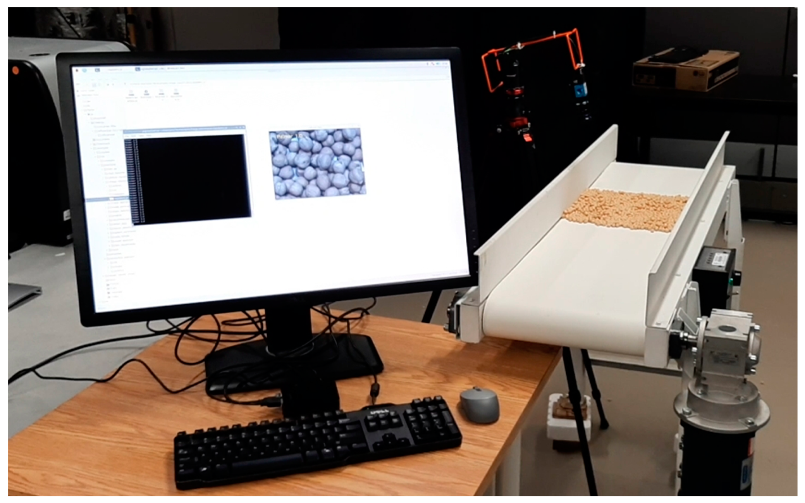
The Tensorflow Lite model was deployed on the Raspberry Pi 4 through a script written in Python that provides basic information, including the real-time prediction of chickpea variety and the percentage of prediction accuracy. The script takes real-time images as input and feeds them one by one to the TFLite model to process them. The model provides a set of confidence scores, which represent the probability of the image belonging to different categories. Then, the script will select the index corresponding to the highest confidence score and present the image along with the label associated with that index. The experimental arrangement for model deployment using the Raspberry Pi 4 is given in Figure 5.

3. Results and Discussion

3.1. Performance of the Models

The performance of the models is displayed in Figure 6. It is vital to monitor the progress of training a deep learning network. The training metrics for each iteration are shown in the training graphs (Figure 6). This visualisation not only displays the changes in network accuracy as the network is trained but it also displays any overfitting of the training data [9]. Figure 6 shows the classification accuracy and cross-entropy loss for the best overall classification accuracy of the pre-trained CNN networks. The holdout validation monitors the training progress and assists in model optimisation. The variation between their training and validation accuracy is negligible, which indicates the model has generalised well enough on the training dataset and performed well on the validation dataset. The figures revealed that NASNet Mobile (Figure 6a), MobileNetV3 (Figure 6b), and EfficientNetB0 (Figure 6c) appeared to have comparable outcomes. The models achieved validation accuracy values that were higher than their training accuracy (

Table 7. Training, validation, and testing results of the three models for chickpea varietal classification.

Model	Training		Validation		Testing		Time Per Image (ms)
	Loss	Accuracy	Loss	Accuracy	Loss	Accuracy
NasNet-A (mobile)	0.499	0.946	0.459	0.959	0.455	0.968	38.36
MobileNetV3	0.465	0.966	0.427	0.981	0.425	0.990	26.82
EfficientNetB0	0.495	0.950	0.442	0.977	0.426	0.981	42.86

) and the figures indicated no overfitting, with the models converging within five epochs. Further, when the model was trained beyond five epochs, it resulted in model overfitting and poor accuracy.

The analysis of Table 7 indicated that the test accuracy obtained with NasNet-A, MobileNetV3, and EfficientNetB0 was 96.82%, 99.09%, and 98.18%, respectively. The high classification accuracy of NasNet can be ascribed to its architecture, where there are only two types of modules or cells. The normal cell extracts features and a reduction cell downsamples the input [27]. The ultimate architecture is created by stacking these cells in a specific pattern, resulting in faster convergence of the network with high accuracy. The good classification accuracy of the MobileNetV3 model can be attributed to their bottleneck residual block, which uses 1 × 1 convolutions to generate a bottleneck. When a bottleneck is used, the number of parameters and matrix multiplications is reduced, which makes the residual blocks as thin as possible in order to maximise depth while using fewer parameters [38]. The original EfficientNet’s basic module is Mobile Inverted Bottleneck Convolution, which contains an expansion convolution to allow for a significantly larger number of channels for depth-wise convolution, resulting in higher accuracy [39]. Furthermore, these networks have a complex architecture and are classified as directed acyclic graph (DAG) networks, which have one layer that receives input from multiple layers and also outputs to multiple layers [9]. Since the chickpea varieties appeared to be very similar, it was critical for the network to learn the complexity among the varieties in order to perform well in classification.

A useful tool for visualising the performance of the CNN networks is the confusion matrix.

Table 8. Confusion matrix of NasNet—A (mobile).

	Consul	Cory	Leader	Orion	Specificity	Sensitivity
Consul	57	0	0	0	1	1
Cory	0	54	0	0	1	1
Leader	0	0	46	4	0.982	0.921
Orion	0	0	3	56	0.975	0.949
Precision	1	1	0.938	0.933

,

Table 9. MobileNetV3 (small) confusion matrix.

	Consul	Cory	Leader	Orion	Specificity	Sensitivity
Consul	61	0	0	0	1	1
Cory	0	58	0	0	1	1
Leader	0	0	50	0	0.988	1
Orion	0	0	2	49	1	0.961
Precision	1	1	0.961	1

and

Table 10. EfficientNetB0 confusion matrix.

	Consul	Cory	Leader	Orion	Specificity	Sensitivity
Consul	49	0	0	0	1	1
Cory	0	50	0	0	1	1
Leader	0	0	54	2	0.988	0.964
Orion	0	0	2	63	0.987	0.969
Precision	1	1	0.964	0.969

display the confusion matrix of the three models used to categorise the four varieties of chickpeas, making it simpler to identify the classes that led to the greatest amount of inaccuracy in the trained models. For a better understanding of the precision and sensitivity (recall) values acquired for each class and model, it is possible to determine the number of images that constitute true positives or false positives for each class. Table 8 of the confusion matrix illustrates this by showing that, of the 50 samples used to categorise CDC-Leader, 46 were correctly identified (TP = 46), whereas 4 were mistakenly classified as CDC Orion (FP = 4). As a result, the CDC Leader’s accuracy was 92% and its false positive rate was 8%. From the confusion tables, it can be observed that the varieties CDC-Leader and CDC-Orion often mispredict each other’s labels, which may be attributed to their close colour shades and subtle differences in seed texture.

Further, the value of the area under the average receiver operating characteristic (ROC) curve, AUC, is provided in Figure 7a for all the three models. It was observed that the AUC values were the highest for the MobileNetV3 and EfficientNetB0 models followed by NasNet-Mobile. The high AUC values are an indicator of the excellent classification performance by the classifier models. Besides, the one-vs.-all classification approach was also conducted with ROC curve and AUC (Figure 7b). Since there are four chickpea varieties, four ROC curves were generated along with their AUC values. For each variety, it was taken as the positive class and the other varieties were jointly grouped as the negative class. The high AUC values in all the three models gives us an indication of the good performance of the models at classifying individual varieties.

It is crucial to determine the time taken by the various models to identify a test image because this reveals the model’s real-time detection speed [40]. For a massive number of convolutional operations, deep CNN needs powerful computing power. The development of small models is urgently needed because smartphones and single-board computers frequently have resource limitations due to their small size. Smaller models can significantly increase detection speed while lowering resource costs. Table 7 shows the length of time required by various CNN models to categorise a single image. On mobile devices and single-board computers, MobileNetV3 outperformed NasNet-A and EfficientNetB0 in terms of speed. NasNet-A mobile (23 MB) and EfficientNetB0 (29 MB) had substantially larger models than MobileNetV3 (1.99 MB), although MobileNetV3′s detection speed (27 ms/image) was quicker than NasNet-A mobile (38 ms/image) and EfficientNetB0 (43 ms/image).

Hence, the classification of the images by MobileNetV3 took the least time among the compared models, making it the most effective model. The model, however, was assessed as a Keras model. Thereafter, the model was enhanced using post-training quantisation and transformed to a TensorFlow Lite model in order for it to be used in edge computing applications like Android mobile and Raspberry Pi 4.

3.2. Performance of the Deployed MobileNetV3 Model

The optimal machine-learning model chosen for deployment was MobileNetV3 based on its relative superior performance. To determine the deployment’s performance, the smartphone’s camera was held on top of a conveyor belt. The chickpea seeds were placed on a conveyor belt operating at a speed of 1 m/min. The smartphone identified each variety in real time, as can be seen in Figure 4. In order to record the results, the results of each frame were saved. As the testing experiment was conducted for 10 s at a speed of 40 fps, we got 400 labels. Thereafter, the confusion matrix was generated from the recorded results (

Table 11. MobileNetV3 (small) confusion matrix on deployed platforms (Android mobile and Raspberry Pi 4).

	Consul	Cory	Leader	Orion	Specificity	Sensitivity
Consul	100	0	0	0	1	1
Cory	0	100	0	0	1	1
Leader	0	0	100	0	1	1
Orion	0	0	0	100	1	1
Precision	1	1	1	1

). A similar approach was taken in the case of Raspberry Pi 4 deployment, where an industrial camera was used to capture the live images of chickpeas, classify them in real time, and display the results on the monitor as given in Figure 5. From Table 11, it is clear that the MobileNetV3 model can successfully classify the chickpea varieties during real-time deployment on both platforms.

4. Conclusions

The present study used a CNN-based model with the transfer-learning approach to distinguish the four different varieties of chickpea. The CNN models used for the study were NasNet-A, MobileNet-V3, and EfficientNet-B0. It was observed that the three models generalised well on the test dataset, with accuracy of 96.82%, 99.09%, and 98.18%, respectively. Further, the optimal MobileNetV3 model was deployed on two platforms, viz., Android mobile and Raspberry Pi 4, by converting trained models into the TensorFlow Lite version. The classification accuracy obtained was 100% on both deployment platforms. Compared to the other models, the MobileNetV3 is lightweight, inexpensive, and requires less time to train. In order to conduct deep learning tasks in rural areas without mobile networks, MobileNetV3-based models are ideal for integration into smartphone apps and IoT devices. However, this study is not applicable to mixtures of varieties and can only accurately identify the chickpea varieties before any mixing. Future studies may involve the application of this automated classification technique to beans and other legumes, and the information can act as a useful resource for bean and legume breeders.