Convergence Check Phase-Field Scheme for Modelling of Brittle and Ductile Fractures

Abstract

The paper proposes a novel staggered phase-field framework for modelling brittle and ductile fractures in monotonic and cyclic loading regimes. The algorithm consists of two mesh layers (displacement and phase field) and a single special-purpose, user-defined finite element, which controls global convergence of the coupled problem and passing of the solution variables between mesh layers. The proposed algorithm is implemented into FE software ABAQUS. For the problem of high cyclic fatigue, a cycle-skipping scheme is also introduced. The proposed methodology is verified on the usual benchmark examples. Small-strain theory is applied, but it has been demonstrated that extension to large strains is straightforward using only the ABAQUS built-in option. The efficiency and stability of the proposed framework was proven by comparison of computational time and the number of iterations per increment in the RCTRL scheme.

1. Introduction

In recent years, modern engineering structures have experienced increased demand for their application, especially in the automotive, aerospace, and energy industries. The most essential requirements in the mechanical design of structures are the prevention of critical fractures and endurance in repeated loading cycles during operation. Hence, the key role of engineers considering the problem is determination of the maximal load capacity of the structure and the number of loading cycles in operation until the fracture in the material occurs. Fracture is the failure mode which denotes splitting of material at two or more parts. This phenomenon can be divided into brittle and ductile fractures based on the constitutive material response. During the fracture, the material undergoes the usual steps, such as crack nucleation, propagation, branching, and total failure. Unlike the brittle fracture, affected by material elasticity, in ductile fractures, a major influence on the material softening is material plasticity. In practice, solving fracture problems represents a cumbersome task, including prediction of complicated crack topology depending on various factors, such as boundary and loading conditions, material properties, and the microstructure. During repeated loading with amplitudes below the load capacity of a material, fractures are frequently a consequence of material fatigue. Material fatigue causes different material failure mechanisms depending on the working conditions and loading. The process of the fatigue fracture can be divided into low- and high-cyclic fatigue regimes. In the former, cyclically loaded mechanical components exhibit fatigue failure after up to 10,000 cycles, while in the latter, fatigue failure occurs after more than 10,000 cycles.

Numerical modelling of the fracture process regarding the fracture description can be divided into discrete and diffusive approaches. In discrete methodologies, a crack is presented as a geometrical discontinuity with a sharp interface. Cohesive zone modelling (CZM), which was first developed by Barenblatt [1] and Dugdale [2] to solve the stress singularity and nonlinear processes ahead of an existing crack, is one of the most used methods for dealing with discrete crack propagation. It is carried out by generalised contact elements that form a narrow band before the crack front and is referred to as the cohesive zone [3]. In the standard approach of CZM finite element implementation as shown in Chandra et al. [4], the results received demonstrate a substantial dependence of the findings on mesh size and orientation during crack formation because the crack propagates along the element edges. Elices et al. [5] conducted a thorough literature analysis of CZMs, including both their benefits and drawbacks. Moreover, remeshing algorithms given in [6,7] and enriched FEM discretization approaches, especially with the extended finite element method (XFEM) [8], were developed to accurately represent various crack topologies. This makes it possible to anticipate the growth of cracks without relying on finite element discretisation. According to Moes et al. [9], XFEM resolves crack tip stress singularities and genuine stress behaviour near the fracture tip with outstanding success; however, a major issue with numerical tracking of the crack discontinuities arises.

In contrast to modelling real crack geometry, diffuse crack modelling approaches include a damage parameter that regulates the material stiffness into the constitutive model of the stress release brought on by the crack formation. De Borst [10] presented a detailed overview. Many continuum damage models preserve the concept of a local continuum theory which does not take into account the material points in the surroundings. According to Aifantis [11], a powerful softening behaviour as a consequence of increasing the damage parameter is followed by an intense strain and damage localisation. Bazant and Belytschko [12] established that the difficulty in the FEM discretisation framework is exhibited by the non-objective results brought on by substantial mesh refinement and alignment dependence. Therefore, non-local [13] and gradient-enhanced continuum techniques [14] have been created to address this issue via the use of length scale parameters, which introduce non-local state variables that typically depend on their local counterparts.

Compared to experiments, which are frequently very expensive, impossible, or unattainable, numerical modelling of a fracture represents a more acceptable solution. Recently, the phase-field method has gained significant attention in the scientific community for modelling of the fracture phenomena. In physics, phase-field fracture models have been established in the Ginzburg–Laudau theory shown in [15], while in mechanics, phase-field fracture models use Griffith’s theory [16] as a base. Griffith proposed the concept of a brittle fracture, introducing an energetic fracture criterion. According to Griffith’s theory, material fails locally upon exceeding a specified fracture energy related to a critical energy release rate. Francfort and Marigo [17] implemented generalisation of the Griffith criterion and the next step toward the phase-field modelling of a fracture, which relies on total energy minimization, consisting of fracture and elastic energy. The proposed methodology can forecast both the initiation of cracks and the emergence of complicated crack patterns. The variational formulation is regularised by Bourdain [18], enabling the determination of the crack evolution and numerical integration. According to [19,20], the phase-field method can effectively be used for solving all governing fracture processes, such as crack initiation, propagation, merging, kinking, and branching. To accurately capture high gradients of the phase-field variable, a very fine mesh is necessary within the diffuse crack region. Unfortunately, this typically results in a significant increase in computing costs compared to FE simulation using the sharp crack interface model with adaptive remeshing [7,21]. Therefore, an adaptive mesh refinement strategy within the phase-field method is increasingly being developed as a solution to this issue [22,23]. The most significant contribution to the phase-field modelling of the quasi-static brittle fracture was achieved by Miehe et al. [24]. Ambati et al. [25] presented a succinct outline of a phase-field brittle fracture. Recently, many papers have been published on the subject of brittle fractures [23,26,27,28] and extend to ductile damage of solids [29]. The proposed research topics include the phase-field method with small-strain [30] and large-strain assumptions [31]. Due to its generality and applicability to a wide variety of problems, the phase-field method has gained increasing popularity as a numerical method for damage modelling. Except for standard fracture problems dealing with metal structures, the phase-field method can also be used for assessment of fatigue fractures in fibre-reinforced composites [32], hyperelastic solids [33], and piezo-electric materials [34]. A detailed overview is given by Wu et al. [35].

Recently, researchers studying phase-field frameworks have dedicated great effort towards the derivation of an extension to fatigue. In [36,37], phase-field fatigue models are presented without physical interpretation or empirical data. A novel approach is presented by Boldrini et al. [38], coupling the additional scalar parameter (which describes the fracture) with thermal and fatigue behaviour. Moreover, Amendola [39] and Caputo and Fabrizio [40] introduced the Ginzburg–Landau form, considering fatigue potential as a material degradation and softening during cyclic loading. In [41], a contribution to energy density is introduced, which is calculated as the sum of additional driving forces during cyclic loading. Carrara et al. [42], Alessi et al. [43], Aldakheel et al. [28], and Seiler et al. [44] proposed the addition of degradation fracture energy based on the stress or strain history. In [45], Hasan et al. include a toughness degradation law depending on the accumulated elastic strain energy density which governs fatigue failure. Furthermore, Golahmar et al. [46] introduced the influence of hydrogen on fatigue. All previously presented research proposals in the field of phase-field fatigue assume linear elastic material behaviour only. On the other hand, Ulloa et al. [47] extended the phase-field fatigue model by considering elastoplastic material behaviour. Unlike the previously mentioned research, Seleš et al. [48] presented a phase-field fatigue numerical framework applicable to both high-cycle and low-cycle regimes based on the three-layered staggered algorithm. As demonstrated by the framework, the key features of Wöhler and Paris law curves are constructed. In [44], material elastoplasticity is empirically included through a local strain approach by Neuber’s rule, while a thermo-mechanical fatigue formulation is introduced by Haveroth et al. [49], incorporating the new degradation function and the Voce-type hardening law. Khalil et al. [50] considered a comparison of different fatigue degradation functions, asymptotic and logarithmic.

One of the greatest problems in the numerical implementation of the currently proposed phase-field models is their robustness. The phase-field numerical framework can be formulated in a monolithic or staggered manner. The monolithic approach calculates phase-field variables and displacements simultaneously. Unfortunately, the disadvantage of a monolithic scheme is instability during fatal crack propagation because of the non-convexity of the regularised free energy functional regarding displacement and phase-field parameters [26]. The non-convexity has been circumvented in several attempts, for example, by the linearization of the elastic part of total energy [22] by restoring the iterative convergence through application of the line-search algorithm with negative and positive parts [51] and by the Newton scheme with Jacobian adjustment [52]. On the other hand, the staggered scheme calculates phase-field variables and displacements separately, restoring, in this way, convexity of the underlying free energy functional. Hence, the weak formulation is decoupled in two equations by the split operator, and it can be solved in an iterative way. However, as demonstrated by numerous researchers, the staggered scheme requires small-scale loading increments to achieve accurate numerical results. Miehe et al. proposed a single iteration staggered procedure [24] which is computationally time consuming and very expensive due to small loading increments. Thus, Bourdain et al. [53] and Duda et al. [54] resolved the problem of small loading increments by incorporating more iterations during one loading increment, constrained by the stopping criterion. In [52], the gradual convergence rate was circumvented by involving over-relaxed alternate minimisation with Newton-type methods [55], while in [25] the proposed solution bypasses this problem by introducing the stopping criterion which normalizes alternation of the strain energy. In contrast, Seleš et al. [27] derived a staggered RCTRL algorithm for brittle fractures with a stopping criterion based on the residual norm, which has been proved as accurate and efficient due to its ability to impose large loading increments. Unfortunately, despite its advantages, the algorithm is computationally exhausting since three mesh layers are required, leading to a large number of unknowns. Therefore, despite tremendous efforts and still increasing popularity of the phase-field methodology, there are still unresolved issues in the phase-field framework. Open questions arise seeking a fast and stable solver strategy, as well as derivation of phase-field models for various physical softening mechanisms.

In this paper, a novel staggered phase-field framework is proposed. Although the three-layer staggered algorithm [27], which is also part of the former research of the authors of this paper, is advantageous by its robustness, this paper proposes a new approach where the third mesh layer is replaced by a single, special-purpose finite element controlling convergence and exchange of the solution variables among the displacement and phase-field mesh layer. The proposed algorithm is implemented into FE software ABAQUS [56] via user subroutines, and it is applicable to general damage phenomena, encompassing brittle and ductile fractures in monotonic and cyclic loading regimes. The proposed methodology assumes a small-strain setting. However, as will be demonstrated, the newly proposed algorithm is easily extended towards large-strain theory. For the problems of the high-cyclic fatigue phenomena, the cyclic skipping technique is utilised.

This paper is organised as follows. Section 2 presents the basic relations of the theoretical background and numerical implementation of the phase-field method. Section 3 deals with numerical implementation in the finite element method. Section 4 describes a novel staggered phase-field algorithm, namely, the convergence check phase-field (CCPF) algorithm, along with cycle-skipping methodology. Section 5 demonstrates the efficiency of the CCPF scheme regarding the usual benchmark problems of brittle, ductile, and fatigue damage for small- and large-strain assumptions. The results obtained by the CCPF scheme are then compared to the results of the RCTRL algorithm, with comparison of CPU time. In the end, Section 6 provides some concluding remarks on the newly proposed scheme.

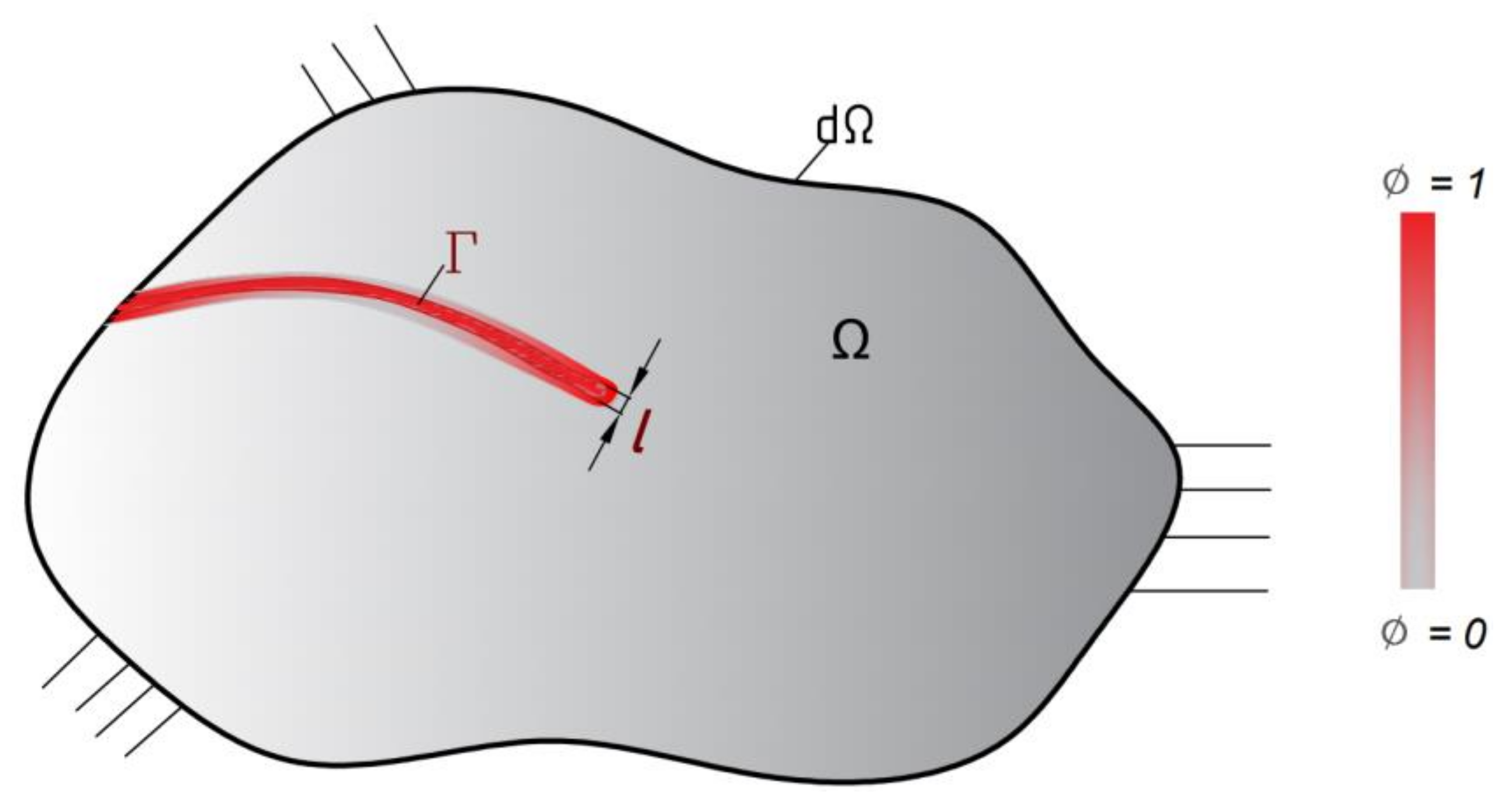
2. Phase-Field Method

As mentioned previously, the phase-field method belongs to the diffusive approaches for describing fractures in deformable bodies. Crack geometry is described by a diffusive zone, where zone width is controlled by the length scale parameter l in the domain Ω (Figure 1). The diffusive zone provides a smooth transition from intact and sound material to fully damaged material, governed by the phase-field scalar parameter $\varphi \left[0,1\right]$, where ϕ = 0 denotes intact material while ϕ = 1 represents fully damaged material. The basic idea of the phase-field method for fracture modelling is based on the variational approach to the fracture process [17]. The governing model is formulated as a minimization problem of the internal energy functional, which consists of the bulk energy ${\mathrm{\Psi }}^{\mathrm{b}}$ stored in the body and the fracture dissipated energy ${\mathrm{\Psi }}^{\mathrm{s}}$, respectively:

$$\mathrm{\Psi }={\mathrm{\Psi }}^{\mathrm{b}}+{\mathrm{\Psi }}^{\mathrm{s}}={\displaystyle {\int }_{\mathrm{\Omega }/\mathrm{\Gamma }}\psi \left(\epsilon \right)}\mathrm{d}\mathrm{\Omega }+{\displaystyle {\int }_{\mathrm{\Gamma }}{G}_{\mathrm{c}}}\mathrm{d}\mathrm{\Gamma }.$$

(1)

Following Griffith’s theory [16], material failure occurs when the material-dependant critical value of fracture energy density $G_{\mathrm{c}}$ is reached. In the phase-field method, the usual problem of tracking discrete fracture surfaces $\mathrm{\Gamma }\left(t\right)$ is omitted through their approximation by the crack density function $\gamma \left(\varphi ,\nabla \varphi \right)$. As mentioned above, crack density function is governed by the incorporation of the length scale parameter l and the phase-field parameter ϕ [53]. In general, the regularised internal energy potential for elastic bodies can be stated as follows:

$$\mathrm{\Psi }\left(\epsilon ,\varphi \right)={\displaystyle {\int }_{\mathrm{\Omega }}\left[g\left(\varphi \right){\psi }_{\mathrm{e}}^{+}\left(\epsilon \right)+{\psi }_{\mathrm{e}}^{-}\left(\epsilon \right)\right]}\mathrm{d}\mathsf{\Omega }+G_{\mathrm{c}}{\displaystyle {\int }_{\mathrm{\Omega }}\gamma \left(\varphi ,\nabla \varphi \right)\mathrm{d}\mathsf{\Omega }.}$$

(2)

In Equation (2), the degradation function $g\left(\varphi \right)$ appears, which degrades material stiffness. In the literature, one of the most popular forms of the degradation function is the quadratic form:

$$g\left(\varphi \right)={\left(1-\varphi \right)}^2.$$

(3)

As can be seen in Equation (2), only the positive part of the strain energy density ${\psi }_{\mathrm{e}}^{+}$ is degraded according to the physically consistent assumption that material loses its stiffness only in tensile state, while in compressive state $\left({\psi }_{\mathrm{e}}^{-}\right)$, crack closure occurs. Hence, in this research, the elastic strain energy density ${\psi }_{\mathrm{e}}$ function is divided into positive and negative parts through a volumetric–deviatoric decomposition [57]. Aside from the volumetric–deviatoric decomposition, other approaches to decomposition are also possible [58]. In this paper, 2 standard forms of the crack density function will be used:

$${\gamma }_{\mathrm{AT}-2}\left(\varphi ,\nabla \varphi \right)=\frac{1}{2}\left[\frac{1}{l}{\varphi }^2+l{\left|\nabla \varphi \right|}^2\right],$$

(4)

proposed in [26,59], referred as AT-2 model, and

$${\gamma }_{\mathrm{TH}}\left(\varphi ,\nabla \varphi \right)=\frac{3}{8\sqrt{2}}\left[\frac{1}{l}2\varphi +l{\left|\nabla \varphi \right|}^2\right],$$

(5)

proposed by Miehe et al. [60], often referred to as the TH model. Furthermore, from the regularised functional in the TH model, a specific fracture energy ${\psi }_{\mathrm{c}}=\frac{3}{8\sqrt{2}}\frac{G_{\mathrm{c}}}{l}$, acting as an energetic barrier preventing the damage evolution, can be derived. The scheme presented in this paper also considers elastoplastic constitutive behaviour of materials prior to fracture. In this case, the bulk energy term of Equation (2) is extended by elastoplastic terms contributing to the total energy potential:

$${\mathbf{\Psi }}^{\mathrm{b}}\left({\mathbf{\epsilon }}^{\mathrm{e}},{\mathbf{\epsilon }}^{\mathrm{p}},\varphi \right)={\displaystyle {\int }_{\mathrm{\Omega }}\left[g\left(\varphi \right){\psi }_{\mathrm{e}}^{+}\left({\mathbf{\epsilon }}^{\mathrm{e}}\right)+{\psi }_{\mathrm{e}}^{-}\left({\mathbf{\epsilon }}^{\mathrm{e}}\right)\right]}\mathrm{d}\mathrm{\Omega }+{\displaystyle {\int }_{\mathrm{\Omega }}g\left(\varphi \right){\psi }_{\mathrm{p}}\left({\mathbf{\epsilon }}^{\mathrm{p}}\right)}\mathrm{d}\mathrm{\Omega },$$

(6)

where ${\mathbf{\epsilon }}^{\mathrm{e}}$ represents the elastic strain tensor, ${\mathbf{\epsilon }}^{\mathrm{p}}$ denotes the plastic strain tensor, while ${\psi }_{\mathrm{p}}\left({\mathbf{\epsilon }}^{\mathrm{p}}\right)$ is the plastic energy potential. After obtaining the internal energy potential, the strong form of the governing equations can be obtained:

$$\nabla \cdot \mathbf{\sigma }+\mathbf{b}=0 \mathrm{in} \mathrm{\Omega },$$

(7)

$$\mathbf{\sigma }\cdot \mathbf{n}=\mathbf{t} \mathrm{on} \partial {\mathrm{\Omega }}_{\mathbf{t}},$$

(8)

$$u=\overline{u} \mathrm{on} \partial {\mathrm{\Omega }}_{\overline{u}},$$

(9)

$$-l^2\Delta \varphi +\left[1+\mathcal{H}\right]\varphi =\mathcal{H} \mathrm{in} \mathrm{\Omega },$$

(10)

$$\nabla \varphi \cdot n=0 \mathrm{on} \partial \mathrm{\Omega }.$$

(11)

Details on the derivation procedure can be found in [29]. In Equations (7)–(11), u represents the displacement vector, b is the volume force vector, t is the surface traction vector, n is the outward-pointing normal vector, and σ is the Cauchy stress tensor. A new parameter introduced in (10) is the history field parameter $\mathcal{H}\left(t\right)$, which prevents nonphysical recovery of material during unloading and constrains the irreversibility of the fracture process according to the second axiom of thermodynamics $\left(\dot{\varphi }\ge 0\right)$. According to [24], it is described as:

$$\mathcal{H}\left(t\right):={\max }_{\tau =\left[0,t\right]}\tilde{D}\left({\psi }_{\mathrm{e}}^{+}\left(\tau \right)\right),$$

(12)

where $\tilde{D}$ represents the crack driving state function. The crack driving state function is derived from the Helmholtz Equation (10), describing the evolution of the phase-field parameter. The crack driving state function for the AT-2 model is:

$${\tilde{D}}_{\mathrm{AT}-2}=\frac{{\psi }_{\mathrm{e}}^{+}+{\psi }_{\mathrm{p}}}{\frac{1}{2}\frac{G_{\mathrm{c}}}{l}},$$

(13)

while for the TH model, the crack driving state function takes the following form:

$${\tilde{D}}_{\mathrm{TH}}=\frac{{\psi }_{\mathrm{e}}^{+}+{\psi }_{\mathrm{p}}}{{\psi }_{\mathrm{c}}}-1.$$

(14)

2.1. Extension of Phase-Field Method to Fatigue

Material fatigue is a phenomenon caused by cyclic loading. The cyclic loading maximum value is usually below the material yield strength and slowly deteriorates the material during loading cycles. After the corresponding number of loading cycles, a fatigue crack initiates. After the initiation stage, stable propagation of the fatigue crack prevails until the critical crack size, when unstable and rapid fatigue crack growth emerges. According to the literature overview, there are many solutions offering extension of the phase-field method towards fatigue problems. In this paper, the approach derived in [48] is adopted. Accordingly, the regularised internal energy potential consisting of (2) and (6) is extended to fatigue, assuming the TH model:

$$\mathrm{\Psi }\left({\epsilon }^{\mathrm{e}},{\epsilon }^{\mathrm{p}},\varphi ,\overline{\psi }\right)={\displaystyle {\int }_{\mathrm{\Omega }}\left\{g\left(\varphi \right)\left[{\psi }_{\mathrm{e}}^{+}\left({\epsilon }^{\mathrm{e}}\right)+{\psi }_{\mathrm{p}}\left({\epsilon }^{\mathrm{p}}\right)\right]+{\psi }_{\mathrm{e}}^{-}\left({\epsilon }^{\mathrm{e}}\right)\right\}}\mathrm{d}\mathrm{\Omega } + {\displaystyle {\int }_{\mathrm{\Omega }}\widehat{F}\left(\overline{\psi }\right)}{\psi }_{\mathrm{c}}\left[2\varphi +l{\left|\nabla \varphi \right|}^2\right]\mathrm{d}\mathrm{\Omega },$$

(15)

introducing the fatigue degradation function $\widehat{F}$. As can be seen from (15), the fatigue degradation function directly affects the energetic threshold and the crack driving state function:

$${\tilde{D}}_{\mathrm{TH}}=\frac{{\psi }_{\mathrm{e}}^{+}+{\psi }_{\mathrm{p}}}{\widehat{F}\left(\overline{\psi }\right){\psi }_{\mathrm{c}}}-1.$$

(16)

The value of the fatigue degradation function is computed by means of the energy density accumulation variable $\overline{\psi }$, which can be formulated as:

$$\overline{\psi }\left(t\right)={\displaystyle {\int }_0^t{\psi }_{\mathrm{e}}\left(t\right)}H\left(-{\dot{\psi }}_{\mathrm{e}}\right)\mathrm{d}t,$$

(17)

where $H\left(-{\dot{\psi }}_e\right)$ denotes the Heaviside function, equal to 1 if ${\dot{\psi }}_e>0$ and equal to 0 if ${\dot{\psi }}_e\le 0$. In this way, the accumulation variable obtains an increase only during unloading, avoiding the influence on the proportional loading cases. Equation (17) can be recast into incremental form for N-th loading cycle:

$$\begin{array}{c}{\overline{\psi }}_N={\overline{\psi }}_{N-1}+\Delta \overline{\psi },\\ \Delta \overline{\psi }={\overline{\psi }}_{N-1}-{\overline{\psi }}_N.\end{array}$$

(18)

The choice of appropriate fatigue degradation functions can be found in Seleš et al. [48], along with necessary properties of the fatigue degradation function. In this paper, 2 forms of fatigue degradation functions have been utilised:

$$\begin{array}{l}{\widehat{F}}_{\mathrm{LCF}}\left(\overline{\psi }\right)={\left(1-\frac{\overline{\psi }}{{\overline{\psi }}_{\infty }}\right)}^2 \mathrm{for} \overline{\psi }\in \left[0,{\overline{\psi }}_{\infty }\right],\\ {\widehat{F}}_{\mathrm{HCF}}\left(\overline{\psi }\right)={\left(\log \frac{{\overline{\psi }}_{\infty }}{\overline{\psi }}\right)}^2 \mathrm{for} \overline{\psi }\in \left[{\overline{\psi }}_{\infty },10{\overline{\psi }}_{\infty }\right].\end{array}$$

(19)

In Equation (19), ${\overline{\psi }}_{\infty }$ represents a material-dependant fatigue parameter.

3. Numerical Implementation into Finite Element Method

Details on the numerical implementation of the phase-field method into the widely used finite element method can be found in [48]. Therefore, only basic relations will be presented herein. Numerical implementation is based on a virtual work principle $\partial W^{\mathrm{ext}}-\partial W^{\mathrm{int}}=0$. According to Equation (15), variation in the internal energy potential is equal to:

$$\delta W^{\mathrm{int}}=\delta \mathrm{\Psi }={\displaystyle {\int }_{\mathrm{\Omega }}\sigma }\delta \epsilon \mathrm{d}\mathrm{\Omega }+{\displaystyle {\int }_{\mathrm{\Omega }}\left\{\frac{\mathrm{d}g\left(\varphi \right)}{\mathrm{d}\varphi }\left({\psi }_{\mathrm{e}}^{+}+{\psi }_{\mathrm{p}}\right)+\widehat{F}(\overline{\psi })G_{\mathrm{c}}\frac{\partial \gamma \left(\varphi ,\nabla \varphi \right)}{\partial \varphi }\right\}}\delta \varphi \mathrm{d}\mathrm{\Omega }.$$

(20)

By discretisation of the virtual work, as explained in [61], we obtain:

$$(F_{\mathrm{ext}}^v-F_{\mathrm{int}}^v)\delta v+\left(F_{\mathrm{ext}}^{\varphi }-F_{\mathrm{int}}^{\varphi }\right)\delta \varphi =0,$$

(21)

where $F_{\mathrm{ext}}^v$ and $F_{\mathrm{ext}}^{\varphi }=0$ denote external force vectors with regard to the displacement field and phase field, respectively. Vector v denotes the displacement vector. In the phase-field method, there are no external nodal forces, while in Equations (7) and (8), the usual external nodal force vector in mechanics is obtained:

$$F_{\mathrm{ext}}^v={\displaystyle \underset{\mathrm{\Omega }}{\int }{N}^{v}b\mathrm{d}\mathrm{\Omega }-{\displaystyle \underset{\partial {\mathrm{\Omega }}_{\mathrm{t}}}{\int }{N}^{v}t}}\mathrm{d}\partial \mathrm{\Omega }.$$

(22)

In Equation (22), N^v is a matrix consisting of shape functions related to the displacement field. $F_{\mathrm{int}}^v$ and $F_{\mathrm{int}}^{\varphi }$ denote internal nodal force vectors regarding to the displacement and phase field, respectively [26]:

$$\begin{array}{l}{F}_{\mathrm{int}}^v={\displaystyle \underset{\mathrm{\Omega }}{\int }{\left(B^v\right)}^{\mathrm{T}}}\sigma \mathrm{d}\mathrm{\Omega },\\ F_{\mathrm{int}}^{\varphi }=-{\displaystyle \underset{\mathrm{\Omega }}{\int }\left\{l^2{\left(B^{\varphi }\right)}^{\mathrm{T}}{B}^{\varphi }\varphi +\left[\left(1+\mathcal{H}\right)N^{\varphi }\varphi -\mathcal{H}\right]N^{\varphi }\right\}}\mathrm{d}\mathrm{\Omega }.\end{array}$$

(23)

The matrix B^v, appearing in the first relation of (23), is the usual strain matrix, consisting of the interpolation polynomial spatial derivatives. $N^{\varphi }$ is the shape function matrix of the phase-field variable. $B^{\varphi }$ is a matrix of spatial gradients of the matrix $N^{\varphi }$, and ϕ is a phase-field vector of the degrees of freedom (DOF). The corresponding stiffness matrices are:

$$\begin{array}{l}{K}^{vv}=-\frac{\partial F_{\mathrm{int}}^v}{\partial v}={\displaystyle \underset{\mathrm{\Omega }}{\int }{\left(B^v\right)}^{\mathrm{T}}}C{B}^v\mathrm{d}\mathrm{\Omega },\\ K^{\varphi \varphi }=-\frac{\partial F_{\mathrm{int}}^{\varphi }}{\partial \varphi }={\displaystyle \underset{\mathrm{\Omega }}{\int }\left\{l^2{\left(B^{\varphi }\right)}^{\mathrm{T}}{B}^{\varphi }+\left[1+\mathcal{H}\right]N^{\varphi }{N}^{\varphi }\right\}}\mathrm{d}\mathrm{\Omega }.\end{array}$$

(24)

K^vv and $K^{\varphi \varphi }$ represent stiffness matrices related to displacement and phase-field DOFs, while C denotes the degraded material tangent matrix. The quantities derived constitute the basic matrices and vectors required for solving the nonlinear finite element equation. As mentioned, there are many approaches to solving the problem of the discretised couple of equations derived. In the next section, a novel staggered approach will be explained.

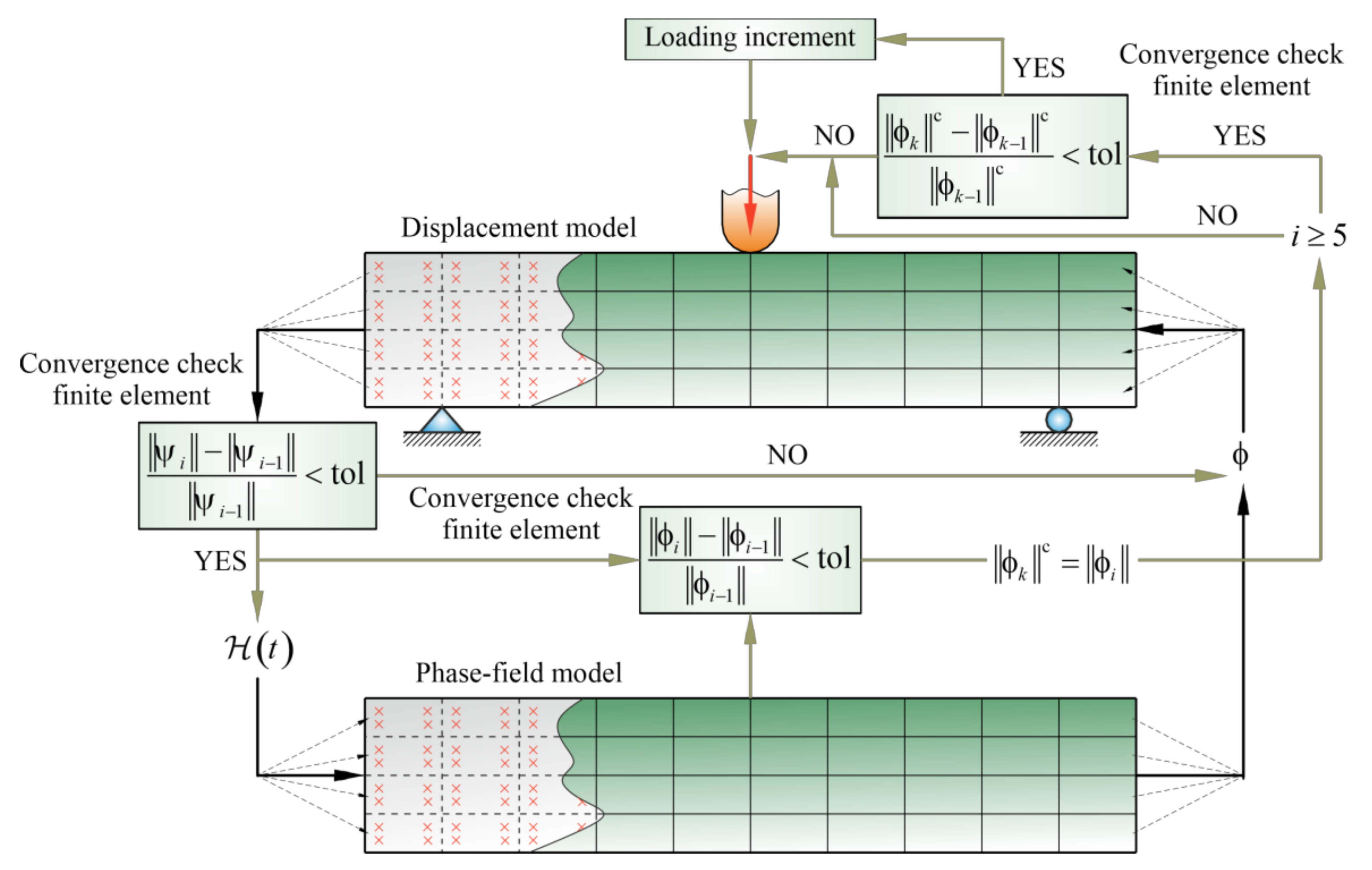
4. Convergence Check Phase-Field Algorithm

The convergence check phase-field (CCPF) algorithm is unlike the many solution algorithms proposed in recent years for dealing with phase-field methodology. Within this manuscript, the proposed methodology references the RCTRL algorithm [27], emphasising the benefits of the newly proposed scheme, since the co-authors of the paper were involved in the derivation and application of the aforementioned framework. One great distinction is the number of mesh layers. In the CCPF algorithm, two meshes are sufficient (displacement and phase field), as in most staggered frameworks. As the name states, the CCPF algorithm relies on the insurance of the convergence of the first mesh layer prior to the transfer of the corresponding variable to the second layer. Basically, during finding the equilibrium in one mesh layer, the solution variable of the other mesh is kept “frozen”, i.e., there is no update to the solution variables in the other layer. This “freezing” approach is standard in the return-mapping algorithm for plasticity problems. A similar approach was proposed in the phase-field methodology in [29] for solving brittle and ductile damage. In this paper, the CCPF framework based on the “freezing” of corresponding solution variables is implemented in commercial FE code ABAQUS through user subroutines for solving problems of brittle and ductile softening in monotonic and cyclic loading regimes (fatigue). For the problem of high-cyclic fatigue, a cycle-skipping scheme was utilised. In the first mesh layer, a UMAT subroutine in combination with the ABAQUS built-in finite elements was employed for the determination of stress, strain, and displacement distribution, allowing implementation of the strain energy density decomposition, required for obtaining physically consistent crack initiation and propagation. The UEL subroutine is employed for implementation of the phase-field in the second mesh layer. More precisely, the first layer consists of quadrilateral CPE4 finite elements, adopting the plane strain assumption. Accordingly, the second mesh layer consists of quadrilateral phase-field user-defined finite elements. The lack of staggered phase-field algorithms creates a need for many loading increments to ensure the correct numerical solution. In the RCTRL scheme, this issue is overwhelmed through application of the third mesh layer consisting of the phase-field elements, allowing the application of large loading increments. Instead of a whole layer of elements, in the CCPF framework, a single finite element, namely, the “convergence check finite element” (CCFE) is employed, thus reducing numerical complexity for one mesh layer compared to the RCTRL scheme. Based on the finite element formulation of the two main mesh layers, CCPF is derived as a quadrilateral finite element. The CCFE checks for the convergence of both mesh layers for variable exchange purposes and controls whether an energy minimum is reached for the appointed loading increment (global equilibrium). The convergence check element is also embedded by the UEL subroutine. The scheme of the CCPF algorithm is presented in Figure 2.

As presented in Figure 2, any problem solved by the CCPF algorithm consists of two mesh layers and one CCFE finite element. It is important to mention that in the CCPF framework, the ABAQUS solver and its convergence measurement tools are utilised, as in usual numerical analysis. On top of the standard ABAQUS convergence checking criterions, the following text explains additional convergence check tools of the CCPF scheme, which ensure the application of larger loading increments. After imposing a loading increment, the first step is finding the equilibrium of the displacement field in the first layer. Through all integration points, for iteration i, strain energy density ψ is stored in a shared field. This field is read by the CCFE to check if the displacement field has obtained convergence according to the relation:

$$\frac{‖{\psi }_i‖-‖{\psi }_{i-1}‖}{‖{\psi }_{i-1}‖}<\mathrm{tol}.$$

(25)

Through iterations, the displacement model also reads from the shared field of the last equilibrated “frozen” values of the phase-field variable ϕ, until criterion (25) is satisfied. During this period, to ensure that there is no change in the values of ϕ, stiffness matrices of the phase-field elements are diagonal matrices with an appointed diagonal value of 10⁸. Once Equation (25) is satisfied, the history variable is transferred into the integration points of the second layer. The stiffness matrix of the phase-field elements takes the form of (24) and new values of the phase-field parameter are obtained and stored in the shared field. If new values of ϕ in the subsequent iteration cause changes in the strain energy density which violate Condition (25), ϕ is again “frozen” until convergence of the displacement field. In every iteration, the CCFE also checks if convergence of the phase-field model has been obtained by the relation:

$$\frac{‖{\varphi }_i‖-‖{\varphi }_{i-1}‖}{‖{\varphi }_{i-1}‖}<\mathrm{tol}.$$

(26)

However, Criterion (26) is not sufficient by itself for further actions in seeking the convergence. Only when both (25) and (26) satisfy their tolerance is a further check of the convergence conducted. If Condition (26) is satisfied (and (25)), the L² norm of the converged phase-field distribution is stored as ${‖{\varphi }_k‖}^{\mathrm{c}}=‖{\varphi }_i‖$, required for control of the convergence of the coupled problem (displacement and phase field). Convergence of the coupled problem is user controlled by controlling the nodal force vector of the CCFE, where the stiffness matrix of the CCFE is again a diagonal matrix with an appointed value 10⁸. Coupled convergence is checked after a minimum of five iterations, which are required for the exchange of variables between layers and confirmation of convergence of each layer separately. Therefore, early in the fifth iteration, if Criterions (25) and (26) are satisfied, the CCFE controls the criterion:

$$\frac{{‖{\varphi }_k‖}^{\mathrm{c}}-{‖{\varphi }_{k-1}‖}^{\mathrm{c}}}{{‖{\varphi }_{k-1}‖}^{\mathrm{c}}}<\mathrm{tol}.$$

(27)

Until satisfaction of Condition (27), the nodal force vector of the CCFE is the unit vector, preventing ABAQUS from pronouncing convergence and forcing additional iterations, even if default ABAQUS convergence criterions are satisfied. In all examples in this paper, the tolerance parameter is set to $\mathrm{tol}=5\cdot {10}^{-5}$ for all three additional convergence conditions. As can be seen, to pronounce convergence of a coupled problem for a corresponding loading increment, local convergence of both layers should be reached, firstly according to the ABAQUS convergence conditions and secondly according to Equations (25) and (26). When additional convergence criterions are satisfied, Equation (27) ensures that relative change between converged states of the phase-field layer is less than the required tolerance. In a physical sense, Condition (27) ensures that for a corresponding loading increment, a global minimum of a two-layer coupling is found and a sufficient number of iterations is calculated, where any potential crack initiation of propagation is captured. ABAQUS subroutines of the CCPF algorithm for the problem of brittle fractures are available for download to all interested readers, where ABAQUS .inp and .for files are provided for the problem of a single-edge notched plate loaded onto tension.

Cycle-Skipping Technique

The phase-field formulation is computationally demanding due to the requirement of dense mesh discretisation which exhibits lengthy computational time. In the case of solving high-cyclic fatigue phenomena, these requirements are multiplied by the number of simulated loading cycles. Therefore, a two-step cycle-skipping technique is embedded into existing numerical routines for the phase-field formulation, relying on the energy accumulation variable $\overline{\psi }$. The first step of skipping occurs during the initial degradation of the bulk material, according to the relation:

$$F\left(\overline{\psi }\right){\psi }_{\mathrm{c}}<\psi .$$

(28)

Prior to damage initiation, constant loading amplitude leads to constant change in the strain energy density $\Delta \psi$. This can be written as:

$$\overline{\psi }={\mathrm{N}}_1\Delta \psi .$$

(29)

For the known fatigue degradation function, (in this paper ${\widehat{F}}_{\mathrm{HCF}}\left(\overline{\psi }\right)$), by inserting (29) into Equation (28), the number of cycles that can be skipped during the first step is computed as:

$${\mathrm{N}}_1=\frac{{\overline{\psi }}_{\infty }}{\Delta \psi }{10}^{-\sqrt{\frac{\psi }{{\psi }_{\mathrm{c}}}}}$$

(30)

To ensure there is no degradation of the material after cycle skipping according to Equation (30), from N₁ cycles which can be skipped, few of them can be subtracted. In this paper, the number of subtracted cycles is two, while the number of jumped cycles N₁ is calculated after the first loading increment. Afterwards, the smallest number of cycles N₁ is used as multiplication factor in accordance with Equation (29) and is imposed in the first unloading increment. After the onset of damage, the second cycle-skipping step is performed. It is based on the extrapolation procedure proposed in [62] and modified for application in the phase-field method in [48]. After established N loading cycles and fatigue variable $\overline{\psi }\left(\mathrm{N}\right)$ for two consecutive loading cycles exhibiting change in the accumulation variables $\Delta {\overline{\psi }}_1$ and $\Delta {\overline{\psi }}_2$, respectively, the number of skipped and extrapolated cycles can be computed by the relation:

$$\Delta {\mathrm{N}}_2=q\frac{\Delta {\overline{\psi }}_1}{\Delta {\overline{\psi }}_1-\Delta {\overline{\psi }}_2}$$

(31)

where q represents a fidelity parameter, which controls the maximum number of jumped cycles allowed. After finding the appropriate number of skipped cycles according to Equation (31), the result is used for extrapolation of the accumulation variable onto a previously achieved value after N cycles as:

$$\overline{\psi }\left(\mathrm{N}+\Delta {\mathrm{N}}_2\right)=\overline{\psi }\left(\mathrm{N}\right)+\Delta {\overline{\psi }}_1\Delta {\mathrm{N}}_2+\frac{1}{2}\left(\Delta {\overline{\psi }}_1-\Delta {\overline{\psi }}_2\right){\left(\Delta {\mathrm{N}}_2\right)}^2$$

(32)

as represented in Figure 3.

The presented two-step procedure is embedded into FE software ABAQUS by means of the subroutine UEXTERNALDB. After first stage of cycle jumping, according to the procedure proposed by the authors, the simulation uses self-checking in a loop to determine whether there is a possibility to extrapolate some loading cycles after the user-controlled number of cycles nFE are computed one-by-one. In this paper, the extrapolation check is performed after every 10 loading cycles. Obviously, the choice of the fidelity parameter q and parameter nFE affects computational time as correctness of the numerical solutions obtained, and therefore, they should be taken with caution. The ABAQUS subroutine of the CCPF algorithm with the cycle-skipping technique is provided by the authors for download, where the problem of high-cyclic fatigue on the CT specimen can be assessed. This is also discussed later in the paper.

5. Numerical Examples

After derivation of the CCPF algorithm, the proposed scheme is verified on the usual benchmark examples from the literature. The verification consists of examples dealing with brittle and ductile fractures in monotonic loading regimes as well as problems of low-cyclic (LCF) and high-cyclic (HCF) fatigue. The results obtained were compared with the RCTRL algorithm. All examples were computed on the Supermicro workstation with 1 TB of RAM, 80 CPUs, and a clock speed of 3.1 GHz. The examples with brittle phenomena were used for the demonstration of the computational speed of the CCPF scheme compared to the RCTRL scheme. Hence, besides the numerical results and crack topology, computational time and number of iterations per increment were compared. After demonstrating the validity of the proposed CCPF framework on the problem of brittle fractures, an example considering elastoplastic behaviour and damage was tested. The last two benchmark problems deal with fatigue where the CT specimen was subjected to LCF and HCF regimes.

5.1. Brittle Fractures

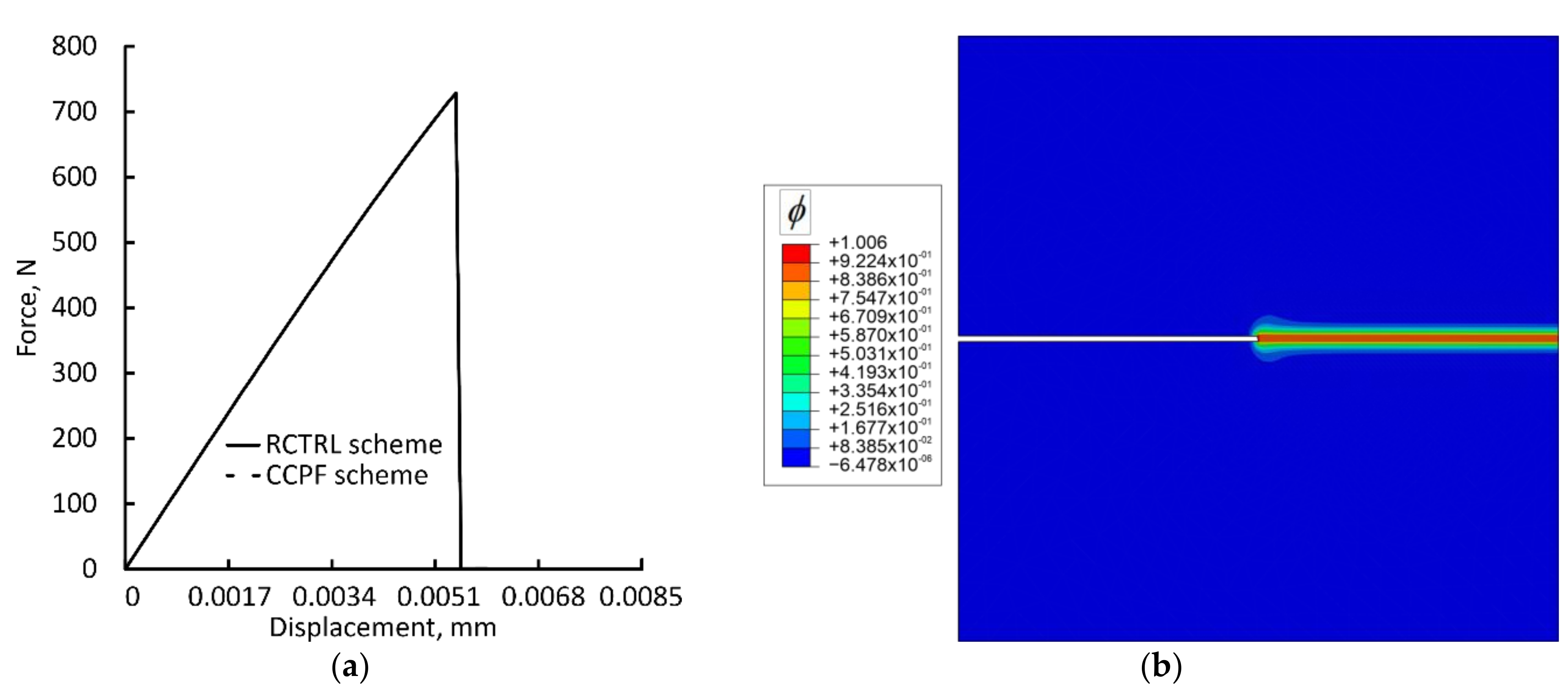
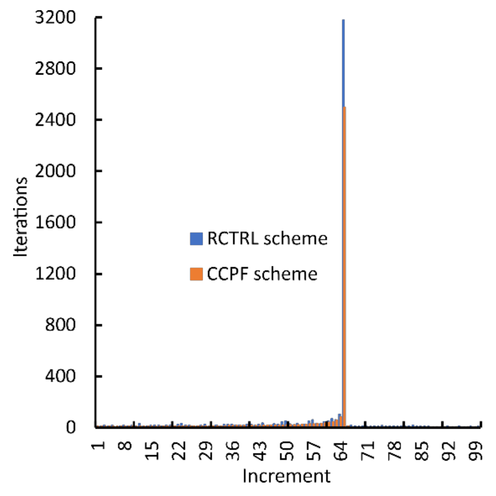
5.1.1. Single-Edge Notched Tensile Test

The first verification problem is a notched plate loaded in tension. Linear elastic material behaviour was adopted with Young’s modulus $E=210 \mathrm{GPa}$ and Poisson’s ratio $\nu =0.3$. The fracture parameters required for phase-field calculations are the critical fracture energy density $G_{\mathrm{c}}=2.7 \mathrm{N}/\mathrm{mm}$ and the length scale parameter $l=0.0075 \mathrm{mm}$. Geometry and boundary conditions are presented in Figure 4.

The model was discretised by 18,868 quadrilateral finite elements in a single layer, with refinement in the expected fracture processing zone (FPZ). Vertical displacement loading $v=0.0085 \mathrm{mm}$ was imposed in 100 increments. The results obtained by two approaches are compared in Figure 5a. As may be observed, the CCPF provides identical results to the RCTRL scheme. Figure 5b presents the distribution of the phase-field variable. It is visible that the correct crack path has been obtained, which is additionally confirmed by the force-displacement curve.

Furthermore, the numerical efficiency of both approaches was compared. Both simulations were conducted with the parallelisation option available in ABAQUS, where four CPUs were utilised. The RCTRL scheme exhibits a wall clock time of 4442 s while the CCPF scheme completes the simulation in 2752 s, which is 38% faster. An additional efficiency comparison of the two frameworks was achieved by comparing iterations per loading increments, as displayed in Figure 6.

According to Figure 6, the CCPF seeks less iterations through increments, especially at the onset of a brittle fracture, demonstrating better stability of the CCPF scheme compared to the RCTRL scheme. Considering the smaller number of degrees of freedom for the same discretisation and less iterations required per increment, the CCPF framework is computationally more efficient, providing faster numerical solutions.

5.1.2. Single-Edge Notched Shear Test

The next verification problem is again a notched plate, now loaded to shear. Material and phase-field parameters are taken from the previous example. Boundary conditions are presented in Figure 7a. For this loading case, the model was discretised by 26,914 finite elements in a single layer, with refinement in the expected FPZ. Horizontal displacement loading $u=0.013 \mathrm{mm}$ was imposed in 100 increments. The results obtained by two approaches are compared in Figure 7b.

As presented in Figure 7b, there are slight discrepancies in the force-displacement dependency of the two frameworks. The general character of the curves is the same in both the pre-peak and post-peak regimes. The latter is also demonstrated by the crack path represented in Figure 8.

Regarding the numerical efficiency comparison, both simulations were conducted on the same workstation by parallelisation with four CPUs. The RCTRL scheme completed the analysis in 95,233 s (26.45 h) while the CCPF scheme completed the simulation in 24,262 s (6.74 h), 75% faster. The numerical efficiency of the CCPF is easily demonstrated by comparing iterations per loading increment in Figure 9.

From Figure 9, it can be seen that the CCPF finds equilibrium and crack propagation through increments in considerably smaller numbers of iterations through increments, which once more demonstrates the efficiency of the CCPF scheme and the reduced computational time compared to the RCTRL scheme.

5.1.3. Asymmetric Three-Point Bending Test

The last verification example of brittle fractures is the standard problem of an asymmetrically notched beam with holes, which demonstrates the ability of the CCPF scheme to capture curvilinear crack paths. The material of the specimen was Plexiglas, according to experimental testing [63], with Young’s modulus $E=20.8 \mathrm{GPa}$ and Poisson’s ratio $\nu =0.3$. The phase-field parameters used in the problem were critical fracture energy density $G_{\mathrm{c}}=1 \mathrm{N}/\mathrm{mm}$ and length scale parameter $l=0.025 \mathrm{mm}$. Geometry and boundary conditions are presented in Figure 10.

The specimen was loaded by the force $F=500 \mathrm{N}$ in 10 loading increments and discretised by 321,154 finite elements in the displacement layer, with refinement in the expected FPZ. However, to avoid unwanted crack initiation at the point where loading is imposed, the yellow shaded zone in Figure 10 was discretised by 320,601 phase-field finite elements. Analogous to the previous examples, mesh discretisation was downloaded from the RCTRL download site. The results obtained by two approaches are compared in Figure 11.

In this problem, the Riks solution method was utilised, because according to Figure 11, the force-displacement dependency represents a snap-back problem which cannot be dealt with using the Newton–Raphson solver. As can be seen, both approaches give identical results. The crack path obtained is shown in Figure 12.

As in previous examples, both simulations were conducted at the same workstation. Herein, the parallelisation option with 10 CPUs was used. The RCTRL scheme completed the simulation in 24,384 s (6.77 h) while the CCPF scheme completed the simulation in 13,190 s (3.66 h), 46% faster. Furthermore, Figure 13 represents iterations per increment.

As in previous examples, it can be seen that the CCPF provides faster solutions, and less iterations are required for finding the equilibrium and crack path. From the presented examples, it can be concluded that the CCPF scheme provides correct solutions with shorter computational time compared to the RCTRL scheme. After verification of the CCPF algorithm on brittle fracture problems, the ability of the proposed method to handle ductile fractures is presented.

5.2. Ductile Fractures

The benchmark problem related to verification of the proposed CCPF algorithm in modelling of ductile fractures involves an asymmetrically notched specimen loaded onto tension. For the specific problem, experimental testing was conducted in [29] on the aluminium alloy Al-5005. Geometry and boundary conditions of the numerical model are displayed in Figure 14. Thickness of the specimen was 3 mm. Vertical displacement loading $v=3 \mathrm{mm}$ was imposed in 100 increments. In the numerical model, the symmetry boundary condition was imposed on the xy plane $\left(w=0\right)$.

Elastic material properties of Al-5005 were Young’s modulus $E=70.9 \mathrm{GPa}$ and Poisson’s ratio $\nu =0.34$. The isotropic hardening law was employed, according to the relation:

$${\sigma }_y={\sigma }_y^0+Q_{\infty }\left(1-e^{-b{\epsilon }_{\mathrm{ekv}}^{\mathrm{p}}}\right)$$

(33)

In Equation (33), initial yield stress is ${\sigma }_y^0=113 \mathrm{MPa}$, saturation coefficient $Q_{\infty }=22 \mathrm{MPa}$, and saturation exponent $b=24.5$. ${\epsilon }_{\mathrm{ekv}}^{\mathrm{p}}$ represents equivalent plastic strain. The material parameters are defined according to [29]. It is important to mention that in [29], large-strain elastoplasticity theory was used. Furthermore, in this example a 3D setting was adopted. Hence, the model is discretised by 16,395 hexahedral finite elements, with refinement in the expected FPZ. Regarding phase-field modelling, the TH model was utilised in this example. The critical fracture energy density $G_{\mathrm{c}}=254.66 \mathrm{N}/\mathrm{mm}$ was taken from [29], while length scale parameter used in the example is $l=1 \mathrm{mm}$, different from the literature [29], where the length scale was set to $l=0.3 \mathrm{mm}$. Furthermore, to improve the convergence rate, the line search option available in ABAQUS was activated. All simulations were finished in approximately one hour. The results obtained are displayed in Figure 15.

As can be observed from Figure 15, small-strain elastoplasticity theory is inadequate for this problem. Therefore, large-strain theory was activated in ABAQUS using the NLGEOM option, where the logarithmic strain is computed without any intervention from UMAT. The force-displacement dependency was in better agreement with the experimental investigation compared to the small-strain setting, as can be seen. However, due to differences in tensorial variables used in the constitutive law used in [29] and this paper, discrepancy still exists. To improve agreement of the results, after several attempts, modifications to initial yield stress ${\sigma }_y^0=118 \mathrm{MPa}$, saturation coefficient $Q_{\infty }=32 \mathrm{MPa}$, and length scale $l=0.9 \mathrm{mm}$ were made. With modified parameters, a significant improvement in numerical results was obtained, as demonstrated by Figure 15. Additional changes should be made to result in better agreement, but this is out of the scope of this paper. A contour plot of equivalent plastic strain and phase-field parameters for a loading displacement of 3 mm is displayed in Figure 16, for the case with modified parameters.

Figure 16 demonstrates the physical consistency of the numerical results, which is in good agreement with [29] although with different values. Hence, according to the results in the example, it can be concluded that the CCPF framework is applicable to the problem of ductile damage, not only for small-strain assumptions but also for large-strain elastoplasticity. To switch between different theories, it is only necessary to activate the NLGEOM option in ABAQUS.

5.3. Low Cyclic Fatigue

The next example demonstrates the ability of the proposed CCPF framework to model LCF phenomena. The problem considered is a CT specimen loaded by force. An analogous benchmark example was taken from [48] for verification of the phase-field method in modelling of material fatigue. A phase-field extension to fatigue derived from [48] was adopted, as explained in Section 2.1. Geometry, material properties, and loading were also taken from [48]. The dimensions of the CT specimen along with boundary conditions are shown in Figure 17.

The parameter w was set to $w=30 \mathrm{mm}$, thickness of the specimen was 15 mm, radius of the notch tip was $r=0.08 \mathrm{mm}$, and parameter $a_0$ was $a_0=7.5 \mathrm{mm}$. Boundary conditions were imposed via kinematic constraints, mimicking pins. The material of the specimen was nodular cast iron, according to [64]. Elastic properties were Young’s modulus $E=140 \mathrm{GPa}$ and Poisson’s ratio $\nu =0.3$. Isotropic hardening is described by the saturation law (33). Initial yield stress equals ${\sigma }_y^0=123 \mathrm{MPa}$, saturation coefficient $Q_{\infty }=95 \mathrm{MPa}$, and saturation exponent $b=18$. Aside from isotropic hardening, due to cyclic loading in the plastic regime, kinematic hardening [65] was also exhibited, according to the relation:

$${\alpha }_k=\frac{C_k\left(\sigma -\alpha \right){\epsilon }_{\mathrm{ekv}}^{\mathrm{p}}}{{\sigma }_y\left({\epsilon }_{\mathrm{ekv}}^{\mathrm{p}}\right)}-{\gamma }_k{\alpha }_k{\epsilon }_{\mathrm{ekv}}^{\mathrm{p}}.$$

(34)

In Equation (34), ${\alpha }_k$ represents back stress tensor and $C_k$ and ${\gamma }_k$ are the kinematic hardening modulus and decrease rate of kinematic hardening, respectively. The total value of back stress tensor can be calculated by summation of k back stress tensors. In this example, $k=2$, with parameters $C_1=\mathrm{22,734} \mathrm{MPa}$, ${\gamma }_1=261.8$, $C_2=\mathrm{136,029} \mathrm{MPa}$, and ${\gamma }_2=2113.5$. The specimen was loaded at the reference point of the upper pin by the concentrated force of amplitude $F=6000 \mathrm{N}$ and load ratio $R=0.1$. The numerical model was discretised by 4224 finite elements in a single layer. Mesh discretisation was densified in the expected FPZ. Since the simulation was conducted for approximately half of the possible crack propagation length, mesh refinement was applied only in this part of the CT specimen. The critical strain energy density parameter used in simulation was $G_{\mathrm{c}}=740 \mathrm{N}/\mathrm{mm}$, while length scale was $l=0.1 \mathrm{mm}$. For consideration of fatigue behaviour, the fatigue parameter ${\psi }_{\infty }$ had a value of ${\psi }_{\infty }=5000 \mathrm{MPa}$. The fatigue degradation function ${\widehat{F}}_{\mathrm{LCF}}$ was used for the degradation of $G_{\mathrm{c}}$ according to Equation (19). Since this example deals with LCF phenomena and material elastoplasticity, cycle skipping was omitted. Furthermore, the line search option was activated for easier convergence of the solver. For better visualisation and numerical efficiency, the element deletion option available in ABAQUS was also utilised in this problem. Hence, all finite elements which exhibit values of phase-field variables $\varphi \ge 0.95$ in all integration points were deleted. The fatigue crack propagation through loading cycles is displayed in Figure 18.

The crack path obtained through cycles is correct, and further verification of the crack propagation can be achieved by comparison with [48], where crack propagation after the same number of loading cycles is displayed. In addition, Figure 19 represents lower and upper displacement amplitude of the reference point of the top pin through loading cycles.

From Figure 19, it can be concluded that after 13,000 loading cycles accelerated crack propagation is expected, leading to the complete fracture of the specimen based on the gradient of the upper displacement amplitude of the top pin. For the problem presented here, the computation time is approximately 18 h.

5.4. High Cyclic Fatigue

The final example demonstrates the ability of the CCPF framework to model HCF phenomena. The CT specimen from the LCF problem presented in Figure 17 is used herein, similar to [48]. The material of the specimen was steel, where only elastic properties were accounted for. Young’s modulus was $E=210 \mathrm{GPa}$ and Poisson’s ratio $\nu =0.3$. For this problem, the specimen was loaded at the reference point of the upper pin by the concentrated force of amplitude $F=400 \mathrm{N}$ and load ratio $R=0$. The specimen was discretised by 29,112 finite elements in a single layer, which is a considerably greater number of finite elements than in the LCF problem. However, in this example, mesh discretisation was densified in the expected FPZ throughout the entire length of the specimen. The critical strain energy density parameter used in the simulation was $G_{\mathrm{c}}=5000 \mathrm{N}/\mathrm{mm}$ while the length scale was $l=0.1 \mathrm{mm}$. The fatigue parameter was set to ${\psi }_{\infty }=50 \mathrm{MPa}$. The logarithmic fatigue degradation function ${\widehat{F}}_{\mathrm{HCF}}$ was used for degradation of $G_{\mathrm{c}}$ according to Equation (19). To speed up computation time, the two-step cycle-skipping technique was tested in this example. In the first stage of cycle skipping, 2504 cycles were jumped prior to any degradation of material, according to Relation (30). In the second stage of cycle skipping, the possibility of the extrapolation procedure occurring was checked every 10th loading cycle by setting the parameter nFE = 20 (10 loading and 10 unloading increments). Two values of relative error parameters, q = 5 and q = 25, were tested. Furthermore, depending on the number of skipped cycles in the first stage, the maximum allowed number of extrapolated cycles was determined. This is a security mechanism because in the early stage of damage development, an unphysically large number of extrapolated cycles can be obtained via Equation (31). Hence, for the example considered, the maximum allowed number of extrapolated cycles was 1000. This is the author-defined value based on experience with the cycle-skipping technique (it was chosen as a round number in the range of 30–50% of stage-one skipped cycles). As in the previous problem, the element deletion option was utilised with a threshold limit of ϕ ≥ 0.95 in all integration points for deletion of the element. The displacement of the top pin through loading cycles with insight into extrapolated cycles is displayed in Figure 20.

As shown in Figure 20, extrapolation of the fatigue variable $\overline{\psi }$ is at the highest degree at the beginning of the simulation for both values of relative error parameter q when the initial fatigue crack develops. The first 20,000 loading cycles are extrapolated by the maximum allowed number. Afterwards, a sudden decrease is observable. Setting a greater limit on the maximum allowable extrapolated cycle number could increase computational speed, but as can be seen from Figure 20, the maximum number of extrapolated cycles is exhibited only at the very beginning of the simulation. In the continuation of the simulation, extrapolation is driven by the value of the relative error. In that sense, for $q=5$, after approximately 30,000 loading cycles there is no extrapolation at all. Therefore, the results obtained herein are considered as relevant since fatigue crack propagation is computed cycle-by-cycle, except the early initiation. With the increase in the relative error parameter to $q=25$, an increase in extrapolated cycles is exhibited, as expected. However, after reaching approximately 50,000 loading cycles, number of extrapolated cycles drops to $\approx 20$ extrapolated cycles and preserves a steady value until the final fatigue fracture. Comparison of the displacement at the top pin for both values of the relative error parameter is presented in Figure 21.

From Figure 21, it can be concluded that the increase in error parameter q and greater extrapolation of fatigue variable $\overline{\psi }$ leads to faster development of the fatigue crack and earlier fatigue fracture. However, differences in the number of cycles until the final fracture are small and acceptable considering the contribution of computational time saving. For error parameter value $q=5$, the fatigue fracture occurs after 195,700 loading cycles, while for $q=25$, the final fracture occurs after 191,600 loading cycles. This shows a difference of 2% on the result. Importantly, the simulation for error parameter value $q=5$ was finished in 23.4 days, while for $q=25$, simulation was over in 6.5 days, which was 72% faster than the reference simulation. To gain an insight, for $F=200 \mathrm{N}$ and $q=25$, a fatigue fracture emerges after 765,800 loading cycles, which is computed in 21 days. Additionally, the referent simulation is calculated with slight cycle skipping. The complete cycle-by-cycle simulation requires even more computational time, which brings a reduced computational time by controlled extrapolation to an even greater extent. With further increase in the error parameter q, shorter computational time can be achieved but at the expense of accuracy of the results. The propagation of the fatigue crack in several stages is displayed on the CT specimen in Figure 22.

The crack path observable in Figure 22 is in accordance with the expectation. From Figure 22a it can be noticed that the fatigue crack initiates after ≈26,000 loading cycles, which is also the moment when number of allowed extrapolated cycles experiences significant collapse (Figure 20). The crack propagates slowly until approximately 140,000 loading cycles, when the crack propagation still stable but with a higher crack growth rate, which is demonstrated by Figure 22c,d. Then, after 195,000 loading cycles, unstable crack growth emerges, which is observable in Figure 22d. Based on the results of the example, it can be concluded that the CCPF scheme provides correct solutions for HCF problems, and application of the cycle-skipping methodology provides significantly shorter computational time compared to cycle-by-cycle simulations.

6. Conclusions

The paper proposes a novel convergence check phase-field staggered scheme for fracture modelling using a phase-field method. This novel methodology can be considered as a continuation of the previously published work related to the phase-field method, where the three-layer RCTRL scheme was proposed and demonstrated as very efficient, alleviating the usual drawbacks of staggered schemes. In this work, the computational burden caused by three dense mesh layers is avoided, since only a single, user-defined convergence check finite element (CCFE) checks for the global convergence of the coupled problem and replaces the third mesh of the RCTRL scheme. Aside from controlling global convergence, the CCFE also controls solution variables passing from one mesh layer to another. Unlike most staggered frameworks which pass solution variables between layers in every iteration, in the CCPF algorithm, the strain energy density history variable is passed to the phase-field layer only when convergence of the displacement layer is satisfied. The proposed methodology is derived from the adopting plane strain and 3D setting. The efficiency of the algorithm was demonstrated by comparison with the RCTRL scheme, where the CCPF algorithm has shown faster computational time and a substantially smaller number of iterations required during crack evolution. The CCPF scheme was implemented into FE software ABAQUS by means of the user subroutines UMAT and UEL. The framework was tested by solving problems of brittle and ductile fractures in monotonic loading regimes. Most of the examples assume a small-strain setting, but it has been demonstrated that the ABAQUS extension towards large-strain theory can be easily applied using the NLGEOM option, giving more accurate results for the ductile damage phenomena. Aside from monotonic loading, validity of the CCPF scheme was tested on problems dealing with low and high cyclic fatigue. An increase in speed for simulations of fatigue problems was provided by the cycle-skipping technique relying on the extrapolation of the fatigue variable, embedded by means of the user subroutine UEXTERNALDB. Additionally, the CCPF framework utilises ABAQUS built-in advanced options, such as line search for convergence improvement and element deletion for better visualization of the damage and numerical efficiency. All interested readers can download routines (.for file) of the CCPF scheme and cycle-skipping technique proposed by the authors and .inp files of the benchmark examples.

References

1. Barenblatt, G.I. The mathematical theory of equilibrium cracks in brittle fracture. Adv. Appl. Mech. 1962, 7, 55–129. [Google Scholar]
2. Dugdale, D.S. Yielding of steel sheets containing slits. J. Mech. Phys. Solids 1960, 8, 100–104. [Google Scholar] [CrossRef]
3. Park, K.; Paulino, G.H. Cohesive Zone Models: A Critical Review of Traction-Separation Relationships Across Fracture Surfaces. Appl. Mech. Rev. 2011, 64, 20. [Google Scholar] [CrossRef]
4. Chandra, N.; Li, H.; Shet, C.; Ghonem, H. Some issues in the application of cohesive zone models for metal-ceramic interfaces. Int. J. Solids Struct. 2002, 39, 2827–2855. [Google Scholar] [CrossRef]
5. Elices, M.; Guinea, J.; Gomez, G.V.; Planas, J. The cohesive zone model: Advantages, limitations and challenges. Eng. Fract. Mech. 2002, 69, 137–163. [Google Scholar] [CrossRef]
6. Tradegard, A.; Nilsson, F.; Ostlund, S. FEM-remeshing technique applied to crack growth problems. Comput. Methods Appl. Mech. Eng. 1998, 160, 115–131. [Google Scholar] [CrossRef]
7. Ingraffea, A.R.; Saouma, V. Numerical Modeling of Discrete Crack Propagation in Reinforced and Plain Concrete; Springer: Dordrecht, The Netherlands, 1985. [Google Scholar]
8. Dolbow, J.; Moes, N.; Belytschko, T. Discontinuous enrichment in finite elements with a partition of unity method. Finite Elem. Anal. Des. 2000, 36, 235–260. [Google Scholar] [CrossRef]
9. Moes, N.; Gravouil, A.; Belytschko, T. Non-planar 3D crack growth by the extended finite element and level sets—Part I: Mechanical model. Int. J. Numer. Methods Eng. 2002, 53, 2549–2568. [Google Scholar] [CrossRef]
10. De Borst, R. Damage, Material Instabilities, and Failure. In Encyclopedia of Computational Mechanics, 2nd ed.; John Wiley & Sons: Hoboken, NJ, USA, 2004. [Google Scholar]
11. Aifantis, E.C. On the role of gradients in the localization of deformation and fracture. Int. J. Eng. Sci. 1992, 30, 1279–1299. [Google Scholar] [CrossRef]
12. Bazant, Z.P.; Belytschko, T.B. Wave-propagation in a strain-softening bar—Exact solution. J. Eng. Mech.-Asce 1985, 111, 381–389. [Google Scholar] [CrossRef] [Green Version]
13. Bazant, Z.P.; Pijaudiercabot, G. Nonlocal continuum damage, localization instability and convergence. J. Appl. Mech.-Trans. Asme 1988, 55, 287–293. [Google Scholar] [CrossRef]
14. Peerlings, R.H.J.; de Borst, R.; Brekelmans, W.A.M.; de Vree, J.H.P. Gradient enhanced damage for quasi-brittle materials. Int. J. Numer. Methods Eng. 1996, 39, 3391–3403. [Google Scholar] [CrossRef]
15. Hakim, V.; Karma, A. Laws of crack motion and phase-field models of fracture. J. Mech. Phys. Solids 2008, 57, 342–368. [Google Scholar] [CrossRef] [Green Version]
16. Griffith, A.A.; Taylor, G.I.V.I. The phenomena of rupture and flow in solids. Philos. Trans. R. Soc. Lond. Ser. A Contain. Pap. A Math. Phys. Character 1921, 221, 163–198. [Google Scholar] [CrossRef] [Green Version]
17. Francfort, G.A.; Marigo, J.J. Revisiting brittle fracture as an energy minimization problem. J. Mech. Phys. Solids 1998, 46, 1319–1342. [Google Scholar] [CrossRef]
18. Bourdin, B.; Francfort, G.A.; Marigo, J.-J. Numerical experiments in revisited brittle fracture. J. Mech. Phys. Solids 2000, 48, 797–826. [Google Scholar] [CrossRef]
19. Miehe, C.; Aldakheel, F.; Raina, A. Phase field modeling of ductile fracture at finite strains: A variational gradient-extended plasticity-damage theory. Int. J. Plast. 2016, 84, 1–32. [Google Scholar] [CrossRef]
20. Molnar, G.; Gravouil, A.; Molnár, G. 2D and 3D Abaqus implementation of a robust staggered phase-field solution for modeling brittle fracture. Finite Elem. Anal. Des. 2017, 130, 27–38. [Google Scholar] [CrossRef] [Green Version]
21. Soghrati, S.; Xiao, F.; Nagarajan, A. A conforming to interface structured adaptive mesh refinement technique for modeling fracture problems. Comput. Mech. 2017, 59, 667–684. [Google Scholar] [CrossRef]
22. Heister, T.; Wheeler, M.F.; Wick, T. A primal-dual active set method and predictor-corrector mesh adaptivity for computing fracture propagation using a phase-field approach. Comput. Methods Appl. Mech. Eng. 2015, 290, 466–495. [Google Scholar] [CrossRef] [Green Version]
23. Nagaraja, S.; Elhaddad, M.; Ambati, M.; Kollmannsberger, S.; De Lorenzis, L.; Rank, E. Phase-field modeling of brittle fracture with multi-level hp-FEM and the finite cell method. Comput. Mech. 2019, 63, 1283–1300. [Google Scholar] [CrossRef] [Green Version]
24. Miehe, C.; Hofacker, M.; Welschinger, F. A phase field model for rate-independent crack propagation: Robust algorithmic implementation based on operator splits. Comput. Methods Appl. Mech. Eng. 2010, 199, 2765–2778. [Google Scholar] [CrossRef]
25. Ambati, M.; Gerasimov, T.; De Lorenzis, L. A review on phase-field models of brittle fracture and a new fast hybrid formulation. Comput. Mech. 2015, 55, 383–405. [Google Scholar] [CrossRef]
26. De Lorenzis, L.; Gerasimov, T. Numerical Implementation of Phase-Field Models of Brittle Fracture BT. In Modeling in Engineering Using Innovative Numerical Methods for Solids and Fluids; De Lorenzis, L., Düster, A., Eds.; CISM International Centre for Mechanical Sciences, Springer International Publishing: Cham, Switzerland, 2020; Volume 599, pp. 75–101. [Google Scholar] [CrossRef]
27. Seleš, K.; Lesičar, T.; Tonković, Z.; Sorić, J. A residual control staggered solution scheme for the phase-field modeling of brittle fracture. Eng. Fract. Mech. 2019, 205, 370–386. [Google Scholar] [CrossRef]
28. Aldakheel, F.; Schreiber, C.; Müller, R.; Wriggers, P. Phase-Field Modeling of Fatigue Crack Propagation in Brittle Materials. In Current Trends and Open Problems in Computational Mechanics; Springer Nature: Cham, Switzerland, 2022; p. 15. [Google Scholar]
29. Ambati, M.; Gerasimov, T.; De Lorenzis, L. Phase-field modeling of ductile fracture. Comput. Mech. 2015, 55, 1017–1040. [Google Scholar] [CrossRef]
30. Yin, B.; Kaliske, M. A ductile phase-field model based on degrading the fracture toughness: Theory and implementation at small strain. Comput. Methods Appl. Mech. Eng. 2020, 366, 113068. [Google Scholar] [CrossRef]
31. Levitas, V.I.; Warren, J.A. Phase field approach with anisotropic interface energy and interface stresses: Large strain formulation. J. Mech. Phys. Solids 2016, 91, 94–125. [Google Scholar] [CrossRef] [Green Version]
32. Tan, W.; Martínez-Pañeda, E. Phase field predictions of microscopic fracture and R-curve behaviour of fibre-reinforced composites. Compos. Sci. Technol. 2021, 202, 108539. [Google Scholar] [CrossRef]
33. Mandal, T.K.; Gupta, A.; Nguyen, V.P.; Chowdhury, R.; de Vaucorbeil, A. A length scale insensitive phase field model for brittle fracture of hyperelastic solids. Eng. Fract. Mech. 2020, 236, 107196. [Google Scholar] [CrossRef]
34. Abdollahi, A.; Arias, I. Phase-field modeling of crack propagation in piezoelectric and ferroelectric materials with different electromechanical crack conditions. J. Mech. Phys. Solids 2012, 60, 2100–2126. [Google Scholar] [CrossRef] [Green Version]
35. Wu, J.Y.; Nguyen, V.P.; Nguyen, C.T.; Sutula, D.; Sinaie, S.; Bordas, S.P.A. Phase-field modeling of fracture. Adv. Appl. Mech. 2020, 53, 1–183. [Google Scholar] [CrossRef]
36. Hosseini, Z.S.; Dadfarnia, M.; Somerday, B.P.; Sofronis, P.; Ritchie, R.O. On the Theoretical Modeling of Fatigue Crack Growth. J. Mech. Phys. Solids 2018, 121, 341–362. [Google Scholar] [CrossRef]
37. Branco, R.; Antunes, F.V.; Costa, J.D. A review on 3D-FE adaptive remeshing techniques for crack growth modelling. Eng. Fract. Mech. 2015, 141, 170–195. [Google Scholar] [CrossRef]
38. Boldrini, J.L.; de Moraes, E.A.B.; Chiarelli, L.R.; Fumes, F.G.; Bittencourt, M.L. A non-isothermal thermodynamically consistent phase field framework for structural damage and fatigue. Comput. Methods Appl. Mech. Eng. 2016, 312, 395–427. [Google Scholar] [CrossRef]
39. Amendola, G.; Fabrizio, M.; Golden, J.M. Thermomechanics of damage and fatigue by a phase field model. J. Therm. Stress. 2016, 39, 487–499. [Google Scholar] [CrossRef] [Green Version]
40. Caputo, M.; Fabrizio, M. Damage and fatigue described by a fractional derivative model. J. Comput. Phys. 2015, 293, 400–408. [Google Scholar] [CrossRef]
41. Schreiber, C.; Kuhn, C.; Müller, R.; Zohdi, T. A phase field modeling approach of cyclic fatigue crack growth. Int. J. Fract. 2020, 225, 89–100. [Google Scholar] [CrossRef]
42. Carrara, P.; Ambati, M.; Alessi, R.; de Lorenzis, L. A framework to model the fatigue behavior of brittle materials based on a variational phase-field approach. Comput. Methods Appl. Mech. Eng. 2020, 361, 29. [Google Scholar] [CrossRef]
43. Alessi, R.; Vidoli, S.; de Lorenzis, L. A phenomenological approach to fatigue with a variational phase-field model: The one-dimensional case. Eng. Fract. Mech. 2018, 190, 53–73. [Google Scholar] [CrossRef]
44. Seiler, M.; Linse, T.; Hantschke, P.; Kastner, M. An efficient phase-field model for fatigue fracture in ductile materials. Eng. Fract. Mech. 2020, 224, 15. [Google Scholar] [CrossRef] [Green Version]
45. Hasan, M.M.; Baxevanis, T. A phase-field model for low-cycle fatigue of brittle materials. Int. J. Fatigue 2021, 150, 106297. [Google Scholar] [CrossRef]
46. Golahmar, A.; Kristensen, P.K.; Niordson, C.F.; Martínez-Pañeda, E. A phase field model for hydrogen-assisted fatigue. Int. J. Fatigue 2022, 154, 106521. [Google Scholar] [CrossRef]
47. Ulloa, J.; Wambacq, J.; Alessi, R.; Degrande, G.; François, S. Phase-field modeling of fatigue coupled to cyclic plasticity in an energetic formulation. Comput. Methods Appl. Mech. Eng. 2021, 373, 113473. [Google Scholar] [CrossRef]
48. Seleš, K.; Aldakheel, F.; Tonković, Z.; Sorić, J.; Wriggers, P. A general phase-field model for fatigue failure in brittle and ductile solids. Comput. Mech. 2021, 67, 1431–1452. [Google Scholar] [CrossRef]
49. Haveroth, G.A.; Vale, M.G.; Bittencourt, M.L.; Boldrini, J.L. A non-isothermal thermodynamically consistent phase field model for damage, fracture, and fatigue evolutions in elasto-plastic materials. Comput. Methods Appl. Mech. Eng. 2020, 364, 112962. [Google Scholar] [CrossRef]
50. Khalil, Z.; Elghazouli, A.Y.; Martínez-Pañeda, E. A generalised phase field model for fatigue crack growth in elastic–plastic solids with an efficient monolithic solver. Comput. Methods Appl. Mech. Eng. 2022, 388, 114286. [Google Scholar] [CrossRef]
51. Gerasimov, T.; De Lorenzis, L. A line search assisted monolithic approach for phase-field computing of brittle fracture. Comput. Methods Appl. Mech. Eng. 2016, 312, 276–303. [Google Scholar] [CrossRef]
52. Wick, T. Modified Newton methods for solving fully monolithic phase-field quasi-static brittle fracture propagation. Comput. Methods Appl. Mech. Eng. 2017, 325, 577–611. [Google Scholar] [CrossRef]
53. Bourdin, B.; Francfort, G.A.; Marigo, J.-J. The Variational Approach to Fracture. J. Elast. 2008, 91, 5–148. [Google Scholar] [CrossRef]
54. Duda, F.P.; Ciarbonetti, Á.A.; Sánchez, P.J.; Huespe, A.E. A phase-field/gradient damage model for brittle fracture in elastic–plastic solids. Int. J. Plast. 2015, 65, 269–296. [Google Scholar] [CrossRef] [Green Version]
55. Farrell, P.E.; Maurini, C. Linear and nonlinear solvers for variational phase-field models of brittle fracture. arXiv 2015, arXiv:1511.08463. [Google Scholar] [CrossRef] [Green Version]
56. Smith, M. ABAQUS/Standard User’s Manual, Version 6.14; Dassault Systèmes Simulia Corp.: Providence, RI, USA, 2014.
57. Amor, H.; Marigo, J.J.; Maurini, C. Regularized formulation of the variational brittle fracture with unilateral contact: Numerical experiments. J. Mech. Phys. Solids 2009, 57, 1209–1229. [Google Scholar] [CrossRef]
58. Van Dijk, N.P.; Espadas-Escalante, J.J.; Isaksson, P. Strain energy density decompositions in phase-field fracture theories for orthotropy and anisotropy. Int. J. Solids Struct. 2020, 196–197, 140–153. [Google Scholar] [CrossRef]
59. Alessi, R.; Ambati, M.; Gerasimov, T.; Vidoli, S.; De Lorenzis, L. Comparison of Phase-Field Models of Fracture Coupled with Plasticity. In Advances in Computational Plasticity: A Book in Honour of D. Roger J. Owen; Oñate, E., Peric, D., de Souza Neto, E., Chiumenti, M., Eds.; Springer International Publishing: Cham, Switzerland, 2018; pp. 1–21. [Google Scholar] [CrossRef]
60. Miehe, C.; Schaenzel, L.-M.; Ulmer, H. Phase field modeling of fracture in multi-physics problems. Part I. Balance of crack surface and failure criteria for brittle crack propagation in thermo-elastic solids. Comput. Methods Appl. Mech. Eng. 2015, 294, 449–485. [Google Scholar] [CrossRef]
61. Kristensen, K.K.; Niordson, F.N.; Martinez-Paneda, E. An assessment of phase field fracture: Crack initiation and growth. Philos. Trans. R. Soc. A 2021, 379, 20210021. [Google Scholar] [CrossRef] [PubMed]
62. Cojocaru, D.; Karlsson, A.M. A simple numerical method of cycle jumps for cyclically loaded structures. Int. J. Fatigue 2006, 28, 1677–1689. [Google Scholar] [CrossRef] [Green Version]
63. Ingraffea, A.R.; Grigoriu, M. Probabilistic Fracture Mechanics: A Validation of Predictive Capability; Cornell University: New York, NY, USA, 1990. [Google Scholar]
64. Čanžar, P.; Tonković, Z.; Bakić, A.; Kodvanj, J. Experimental and Numerical Modelling of Fatigue Behaviour of Nodular Cast Iron. Key Eng. Mater. 2012, 488–489, 182–185. [Google Scholar]
65. Chaboche, J.L. Constitutive equations for cyclic plasticity and cyclic viscoplasticity. Int. J. Plast. 1989, 5, 247–302. [Google Scholar] [CrossRef]
Figure 1. Fracture surface Γ approximated by a phase-field diffusive approach.
Applsci 13 07776 g001
Figure 2. Scheme of the CCPF algorithm.
Applsci 13 07776 g002
Figure 3. Extrapolation-based cycle-skipping scheme.
Applsci 13 07776 g003
Figure 4. Geometry and boundary conditions of a single-edge notched tensile test.
Applsci 13 07776 g004
Figure 5. Single-edge notched tensile test: (a) force-displacement diagram, (b) crack pattern.
Applsci 13 07776 g005
Figure 6. Number of iterations utilised through loading increments for a single-edge notched tensile test.
Applsci 13 07776 g006
Figure 7. Single-edge notched shear test: (a) boundary conditions, (b) force-displacement diagram.
Applsci 13 07776 g007
Figure 8. Crack pattern of a single-edge notched shear test.
Applsci 13 07776 g008
Figure 9. Number of iterations utilised through loading increments for a single-edge notched shear test.
Applsci 13 07776 g009
Figure 10. Geometry and boundary conditions of an asymmetric three-point bending test.
Applsci 13 07776 g010
Figure 11. Force-displacement diagram of an asymmetric three-point bending test.
Applsci 13 07776 g011
Figure 12. Crack pattern of an asymmetric three-point bending test: (a) whole model, (b) crack detail.
Applsci 13 07776 g012
Figure 13. Number of iterations utilised through loading increments for an asymmetric three-point bending test.
Applsci 13 07776 g013
Figure 14. Geometry and boundary conditions of an asymmetrically notched specimen.
Applsci 13 07776 g014
Figure 15. Force-displacement diagram of an asymmetrically notched specimen (Ambati et al. [30].
Applsci 13 07776 g015
Figure 16. Distribution of contours on deformed shape of an asymmetrically notched specimen: (a) equivalent plastic strain, (b) phase-field variable.
Applsci 13 07776 g016
Figure 17. Geometry and boundary conditions of CT specimen.
Applsci 13 07776 g017
Figure 18. Fatigue crack propagation in the LCF regime through cycles: (a) 2000 cycles, (b) 7000 cycles, (c) 10,000 cycles, (d) 13,000 cycles.
Applsci 13 07776 g018
Figure 19. Displacement amplitude of the top pin through cycles in a low cyclic fatigue regime.
Applsci 13 07776 g019
Figure 20. Displacement amplitude of the top pin through loading cycles: (a) q = 5, (b) q = 25.
Applsci 13 07776 g020
Figure 21. Comparison of the displacement amplitude of the top pin for two values of the relative error parameter q.
Applsci 13 07776 g021
Figure 22. Fatigue crack propagation in the HCF regime through cycles: (a) 26,000 cycles, (b) 91,000 cycles, (c) 141,000 cycles, (d) 195,000 cycles.
Applsci 13 07776 g022
Disclaimer/Publisher’s Note: The statements, opinions and data contained in all publications are solely those of the individual author(s) and contributor(s) and not of MDPI and/or the editor(s). MDPI and/or the editor(s) disclaim responsibility for any injury to people or property resulting from any ideas, methods, instructions or products referred to in the content.