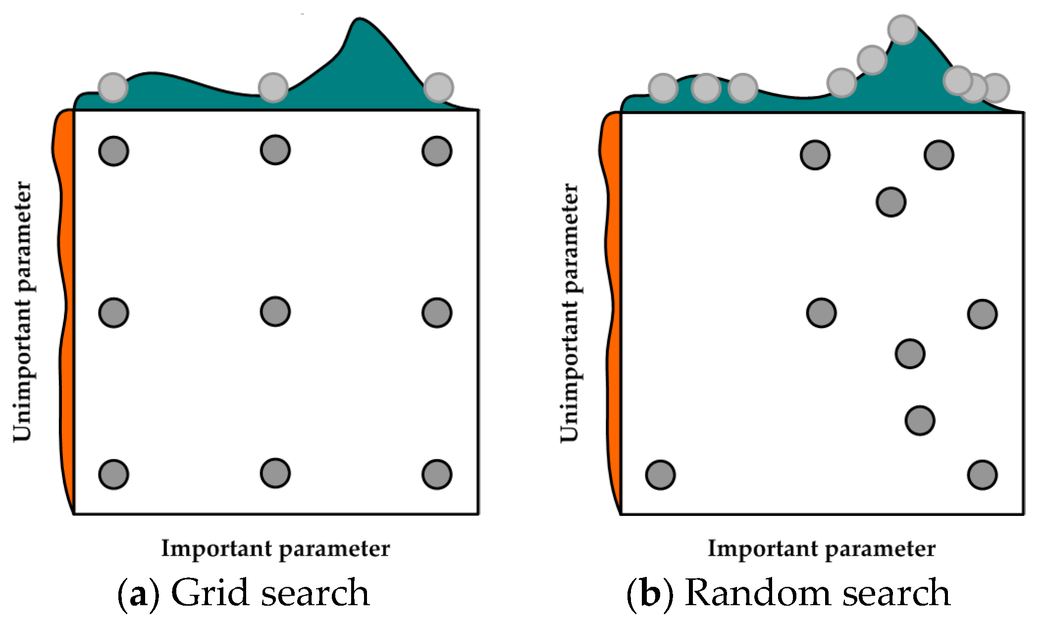
Article

A COP Prediction Model of Hybrid Geothermal Heat Pump Systems based on ANN and SVM with Hyper-Parameters Optimization

1
Enertecunited, Busan 48059, Republic of Korea
2
Institute of Industrial Technology, Yeungnam University, Gyeongsan 38541, Republic of Korea
3
School of Architecture, Yeungnam University, Gyeongsan 38541, Republic of Korea
*
Author to whom correspondence should be addressed.
Appl. Sci. 2023, 13(13), 7771; https://doi.org/10.3390/app13137771
Submission received: 18 May 2023 / Revised: 23 June 2023 / Accepted: 24 June 2023 / Published: 30 June 2023
(This article belongs to the Special Issue Control Methods for Energy Efficiency Technologies in Buildings)

Abstract

:
When the geothermal heat pump system is operated due to an imbalance in the heating and cooling load, the system performance is lowered due to the occurrence of a thermal environment problem in the ground. To solve the performance degradation, a hybrid geothermal heat pump system with an added auxiliary heat source is used. For the efficient operation of the system, it is necessary to check the performance coefficient of the hybrid geothermal system. The coefficient of performance can be monitored based on a mathematical model using a measuring instrument. However, in the case of mathematical models, there are a lot of input data required, and many measurement sensors are required for this. If there is an input factor that is omitted among the necessary input factors, the accuracy of the predicted performance coefficient is lowered or a problem occurs that it is impossible to predict. In this study, we intend to create a model that predicts the coefficient of performance (COP) by using ANNs and SVMs that can accurately predict at low cost using small input factors. Hyper-parameter optimization is performed to increase prediction accuracy in machine learning models. We compared the accuracy of ANN and SVM-based prediction models. In this study, the ANN model showed higher CvRMSE by 5.4% and SVM by 8%. It is expected that the predictive model will be able to be used in the operation of the hybrid geothermal system in the future.

1. Introduction

The operation of a hybrid geothermal heat pump system aims to prevent the performance degradation of a system due to geothermal environmental problems [1,2,3]. This study aimed to reach the maximum coefficient of performance of the entire system by considering the energy of the heat pump and the energy saving of the circulation pump when controlling the flow rate of circulating water on the load side and the heat source side. To this end, it is necessary to monitor the current coefficient of performance according to the operation of a hybrid geothermal heat pump system and predict the coefficient of performance of the next stage. When installing a general geothermal system, a short-term coefficient of performance measurement is performed to check the steady state of the system and long-term coefficient of performance monitoring is not performed. The coefficient of performance monitoring and prediction of the coefficient of performance in the next operation can be confirmed based on a mathematical model using the measured operational data. On the other hand, in the case of a mathematical model, many necessary input factors require many measurement sensors. When an input factor is omitted from the necessary input factors, the accuracy of the predicted performance coefficient is lowered, or an unforeseen problem can occur [4,5].
A machine learning predictive model uses several theoretical techniques to find and predict the relationship between input and output data. Compared to a mathematical model, prediction is possible through relatively few input factors and requires a large amount of data. Various data collections are made using a BAS (Building Automation System) for system operation and monitoring in building facility systems, and it can be used to develop predictive models through machine learning. A machine learning-based prediction model cannot be estimated from data, unlike parameters that are estimated or learned from data and stored as a part of the trained model. The performance of the model is different. Selecting the optimal hyper-parameter is essential for improving the performance of the prediction model. The prediction performance can be improved compared to the initial prediction model. In this study, a machine learning-based coefficient of the performance prediction model was developed through hyper-parameter optimization to predict the coefficient of performance in real-time and the next stage of performance, which is a necessary element for the efficient operation of a hybrid geothermal system [6].

2. Theoretical Analysis

2.1. Hyper-Parameter

A machine learning-based prediction model cannot be estimated from data, unlike parameters that are estimated or learned from data and stored as a part of the trained model. The performance of the model is different. Hyper-parameters are the input values of machine learning and deep learning models and control the model to train generalized inference performance from the target data characteristics. These hyper-parameters are composed of various variables that directly affect the model training performance, such as learning rate, learning rate scheduling method, loss function, number of training iterations, weight initialization method, regularization method, and the number of layers to be stacked.
Selecting the optimal hyper-parameter is essential for improving the performance of a prediction model. The prediction performance can be improved compared to the initial prediction model. In machine learning, each model has a range of hyper-parameters; Table 1 lists the types and descriptions of hyper-parameters.
Hyper-parameters can be optimized using various techniques. The manual search method is where the user calculates the optimal hyper-parameter through repeated execution based on intuition or experience. The random search method is a method to find the optimal combination by repeatedly extracting random values within the range, setting the minimum and maximum values of each hyper-parameter, and narrowing the extraction range based on the previously extracted and evaluated results. Hence, Bayesian optimization can optimize the hyper-parameters. Figure 1 shows the conceptual diagram of grid search and random search methods among hyper-parameter optimization methods.

2.2. COP Prediction Model Based on Machine Learning

For optimal control and energy saving of HVAC systems, it is necessary to accurately predict the coefficient of performance of a geothermal heat pump system [7]. For the coefficient of performance of the heat pump, there are theoretical calculations through mathematical models, short-term monitoring through simulations, long-term monitoring through measuring instruments [8,9], or predictive model development through machine learning [10,11]. Theoretical calculations using a mathematical model require a large number of input values, as shown in Figure 2. Hence, the model is expensive due to the need for various measuring equipment to measure it. Long-term on-site monitoring is the most accurate and reliable way of providing operational management guidance to maintain proper operation. On the other hand, the long-term monitoring method is expensive and time-consuming.
A simulation is performed using commercial software, such as TRNSYS and theoretical models. The simulation results often appear more accurate than experimental field results because the simulation conditions are theoretical and simplified, ignoring real uncertain factors. In the case of a simulation, it requires professional knowledge and information collection on various conditions for the simulation, and it takes considerable time. A performance coefficient prediction through machine learning is a method of expressing the dynamic behavior of a system through measurement data. It does not require a high degree of expertise compared to other methods and does not require the selection of various variables [7,12].
Regarding the prediction of the coefficient of performance of geothermal systems, prediction techniques using mathematical models, such as multiple linear regression (MLR) [13,14], calculation of the coefficient of performance through simulation, and various machine learning models [15,16], such as artificial neural network (ANN)s and support vector machine (SVM)s, have been conducted in previous studies. Table 2 lists the contents of the existing literature research on the coefficient of a performance prediction model using various machine-learning models.
Simon applied MLR to model the COP of a geothermal heat pump but used simulated data. Akhlaghi used a multiple polynomial regression approach to evaluate the effects of the intake air temperature, relative humidity, flow rate, and working air ratio on the COP of a dew point air cooler using simulation data. Park et al. developed MLR and ML neural network models to evaluate the essential parameters for predicting the COP of geothermal heat pump systems in hospital buildings [14]. Nam predicted the coefficient of performance of the geothermal system through a mathematical model, and Benli developed a prediction model using an ANN model with heat pump energy consumption as input [17]. Esen et al. developed a coefficient of the performance prediction model [18].
In the existing coefficient of performance prediction study, the coefficient of performance was predicted using various methods, but the coefficient of the performance prediction was mainly performed by machine learning using the directly related input values used for mathematical calculation of the coefficient of performance, such as power consumption and flow. In addition, things that are difficult to measure during operation or measured through multiple monitoring sensors, such as heat capacity, were used as input values. In addition, the coefficient of the performance prediction model was developed mainly using the data in the limited temperature range provided by the manufacturer or the data limited to the simulation, and studies related to the optimization of hyper-parameters to improve the accuracy of the prediction model are lacking. This study developed a coefficient of a performance prediction model that shows high accuracy at a low cost using the input values that are generally monitored and easy to measure during the operation of a heat pump system. The coefficient of a performance prediction model was developed using the operational data of geothermal systems and measurement data in various temperature ranges through experiments. The accuracy was improved through hyper-parameter optimization.

3. Methodology

Figure 3 shows a flow chart of the development of the performance prediction model. The development of the performance coefficient prediction model proceeds in the order of data collection and preprocessing for predictive model development, input variable selection, initial prediction model development, final prediction model development through hyper-parameter optimization, and prediction performance analysis.
In this study, R studio (Ver. 1.2.1335) has been used for research, and an industrial application was used as a language for data mining and machine learning for developing the predictive model.

3.1. Data Collection and Pre-Processing

A model was developed for predicting the coefficient of performance of a hybrid geothermal heat pump system by collecting data from the target building where the existing geothermal system was installed and operated and data from a test bed equipped with equipment that simulates the geothermal system. The coefficient of performance of the hybrid geothermal heat pump system is equivalent to predicting the coefficient of performance of a geothermal heat pump system. When operating a hybrid geothermal system, the circulating water heat exchanged in the ground undergoes additional heat exchange from an auxiliary heat source, which changes only the temperature entering the heat pump. Hence, a hybrid geothermal system coefficient of the performance prediction model can be developed using the data from the geothermal system. The actual geothermal system operation data were collected through the BAS system for the buildings in which the geothermal system was installed. Table 3 shows an overview of the building for geothermal system operation data collection.
Additional data were collected from the test bed to develop a coefficient of a performance prediction model using the data of various temperature ranges that may occur during geothermal and hybrid geothermal systems operation. Figure 4 shows the configuration of the entire system used in the experiment, and the overview of the heat pump system is listed in Table 4.
The test bed used a constant temperature tank connected to a heat pump to simulate the heat source and load side and the heat source side. It was used as the cooling and heating source and for maintaining the temperature through an air-cooled auxiliary heat source. The load and heat source sides were simulated by connecting a constant temperature tank to a heat pump to supply cooling and heating sources and maintain the temperature through an air-cooled auxiliary heat source. Table 5 outlines the experimental system, and Figure 5 shows the systems installed in the target building.
In both systems, the factors affecting the performance coefficient of the geothermal heat pump, such as inlet and outlet temperature difference, flow rate, and power consumption, were collected for the performance evaluation in both systems, as well as the outside air temperature. Table 6 gives an overview of the operational data collection in both systems.
In the case of a building with a geothermal system installed, data monitored through BAS were collected at a three-hour cycle, and the data from January 1 to 31 December 2018, where data in various temperature ranges among the total collected data were analyzed, were used to predict the coefficient of performance. In the test bed, the inlet/outlet temperature of the heat source and load side at one-minute intervals utilized an RTD (Resistance Temperature Detector) temperature sensor and was stored as a data logger (MV2000). The flow rate was measured through the load and heat source side thermostat system, and the flow meter (FMAG5000) was installed on the water pipeline. The power consumption was measured by installing a watt-hour meter (CW240) on the heat pump. The outside air temperature and humidity were measured, and data were collected through the HOBO U12. Figure 6 shows the measurement items and devices measured in the experiment and Table 7 shows the accuracy of the measurement devices.
For performance evaluation in a broader range of heat source inlet-temperature conditions considering actual operating conditions, each item was measured while changing the heat source inlet temperature in the range of 8.1–26.8 °C during the heating operation and 20–49 °C during the cooling operation. The experiment was carried out as the water in the water tank on the heat source, and the load side was circulated and heated or cooled to the initial set temperature. After opening various valves connecting the heat pump and the water tank on the heat source side to circulate water, the temperature and flow rate of water at the inlet side of the heat pump heat-source-side were set to suit the experimental conditions. Various valves connecting the heat pump and the water tank on the load side were opened to circulate water. The temperature and flow rate of water at the inlet of the load side of the heat pump was set according to the experimental conditions. When a steady state was reached, each measurement item required to derive the heat pump performance coefficient was measured and recorded according to the measurement cycle. Table 8 lists the operational data items collected for the two systems. As for the measurement uncertainty, as shown in Table 9, the uncertainty of the temperature measuring device is 0.2 and the uncertainty of the flow meter is 0.26~0.32.
A large amount of data collected through the heat pump operation in the target building were analyzed to select the input variable by assessing the correlation between the coefficients of performance. An input variable was selected by quantitatively evaluating the relationship with a performance coefficient to be predicted using a Pearson correlation coefficient and a coefficient of determination. The Pearson correlation coefficient was calculated using Equation (1), and the coefficient of determination was calculated as the square of the Pearson correlation coefficient.
r = i = 1 n X i X ¯ Y i Y ¯ i = 1 n X i X ¯ 2 i = 1 n Y i Y ¯ 2
  • r: Pearson correlation coefficient
  • n : Number of data
  • X i : Input data
  • X ¯ : Average of input data
  • Y i : Output data
  • X ¯ : Average of output data
The Pearson correlation coefficient is a number from 1 to −1. As the value of the correlation coefficient approaches 0, the relationship between the input and output data is weaker. The coefficient of determination indicates the correlation between two variables to be measured; a coefficient closer to 1 indicates better performance. The inlet temperature, outlet temperature, load-side inlet temperature, outlet temperature, and outdoor temperature were used as the input. The monitored items with a high correlation coefficient between input data and output data of less than 0.2 and a coefficient of determination of less than 0.04 among the performance coefficient theoretical equation were selected as variables. Table 10 lists the analysis results of the determination coefficient and Pearson correlation coefficient for the input and output data for the selected input variable.
The heat-source-side outlet temperature showed the highest correlation among the input variables, with a Pearson correlation coefficient of −0.76 and a coefficient of determination of 0.58. The outdoor temperature had a Pearson correlation coefficient of 0.32 and a coefficient of determination of 0.10, indicating a relatively small relationship among the input variables.
The data of the input variables, such as the inlet temperature on the heat source side, outlet temperature on the heat source side, load side inlet temperature, load side outlet temperature, and outdoor temperature, are the learning data by deleting the data in the non-operational state of the geothermal system and excluding abnormal data (null) values. (Training data), validation data (Testing data), and evaluation data (Validation data) to generate training data for predictive model development.

3.2. Accuracy Metrics

In this study, to develop an initial predictive model and improve the performance of the initial model, hyper-parameters for each machine learning are selected and set. The predictive model optimization and optimized hyper-parameters were calculated by performance analysis of the predictive model. The predictive model development and performance were analyzed using the parameters applied.
The accuracy was evaluated using the coefficient of variation, the Mean Bias Error (MBE), and the Coefficient of Variation (CV) to evaluate the performance of the predictive model. The MBE means the total error of the predicted value, and the coefficient of variation is a method of analyzing the error through the degree of variance. Using the criteria provided by ASHRAE Guideline 14 (MBE of 10% and Coefficient of variation of the Root Mean Squared Error (CvRMSE) of less than 30%), the accuracy of the prediction model was evaluated, as shown in Equations (2)–(4) below [19,20].
  MBE = i = 1 n P i M i n × 100
  RMSE = i = 1 n P i M i 2 n
C v RMSE = RMSE P ¯ × 100
  • P : Predicted value
  • M : Measured value (or simulation value)
  • n : Number of measured data
  • P ¯ : Average of predicted value

4. COP Prediction Model Development with Hyper-Parameter Optimization

4.1. Initial COP Prediction Model Development

In this study, an initial coefficient of performance prediction model was developed using an ANN and an SVM model to analyze the suitability for predicting the heat pump performance coefficient by machine learning. At this time, each prediction model was developed using the built-in function of R studio. The initial model performance and optimization performance are compared and analyzed. Table 11 shows the statistical analysis of parameters through the random classification of input variables and training data selected for developing the initial coefficient of the performance prediction model [21].
The training data and the validation data were evenly distributed for all parameters. Statistical analysis of the parameters was performed by random classification of the input variables. The training data selected for developing the initial coefficient of the performance prediction model are shown in Table 12. The training and validation data were distributed evenly for all parameters [22].
The initial ANN utilization prediction model was constructed as an ANN model with a structure of one hidden layer and two hidden neurons with input variables. Table 13 lists the structure of the ANN, and Table 14 shows the structure of the initial prediction model of the SVM [23,24].
The performance of the initial prediction model was evaluated based on the coefficient of determination, CvRMSE, and calculation time by comparing the predicted heat pump performance coefficient and the measured heat pump performance coefficient by inputting the test data into the developed prediction model. Table 15 presents the performance evaluation result, and Table 16 lists the calculation time analysis result. The ANN model satisfied the decision coefficient criterion exceeding 0.8 and the CvRMSE criterion. For the SVM, the CvRMSE was 15.9, which satisfied the criterion, but the coefficient of determination did not. The prediction accuracy of the initial model was 17.8% for the ANN model and 15.9% for the SVM, showing that the SVM was higher.
The computation time of the prediction model for the environment to be checked in real-time should be considered, along with the accuracy of the prediction. The ANN terminates the operation when the indicator specifying the error between the measured value and the predicted value reaches a certain level. Table 17 lists the computation time analysis results of the initial coefficient of the performance prediction model developed using ANNs and SVMs.
The ANN model has a shorter computation time than the SVM. A real-time prediction is possible because both models were calculated within one minute. The performance of the initial predictive model was improved by optimizing the structure and parameters of the predictive model.

4.2. Hyper-Parameter Optimization

When developing a machine learning-based prediction model, it cannot be estimated from data, unlike the parameters that are estimated or learned from data and stored as a part of the trained model. The performance of the model was different. It is essential to select the optimal hyper-parameter to improve the performance of the prediction model. The prediction performance can be improved compared to the initial prediction model. Table 17 lists the hyper-parameters analyzed for each machine learning model in this study and the optimization method.
Hyper-parameters can be optimized using a range of techniques. In the manual search method, the user calculates the optimal hyper-parameter through repeated execution based on intuition or experience. The random search method is used to find the optimal combination by repeatedly extracting random values within the range, setting the minimum and maximum values of each hyper-parameter, and narrowing the extraction range based on the previously extracted and evaluated results. Hence, Bayesian optimization optimizes hyper-parameters.

4.2.1. ANN Hyper-Parameter Optimization

In the ANN-based coefficient of the performance prediction model, the learning degree changes according to the number of hidden layers (Hidden Layer, HL) and the number of neurons in the hidden layer (Hidden Neuron, HN). As the number of hidden layers increases, the ANN is called “deep”. In the case of a simple I/O relationship, high learning performance is possible even if the number of hidden layers and neurons is small. It is important to select the number of hidden layers and the number of neurons in the predictive model. In the hyper-parameter range of Table 18, the optimal number of hidden layers and neurons are derived through Bayesian optimization.
Figure 7 shows the prediction model performance analysis according to 100 repetitions of learning. The performance of the performance coefficient prediction model was stabilized at 60 repetitions of learning. After a steady decrease in RMSE up to 40 times, unstable performance was analyzed during 40 to 50 repetitions. This required iterative learning at least 60 times to develop a performance coefficient prediction model using an ANN model.
The optimization of the number of hidden layers and the number of neurons proceeds through two steps. First, the coefficient of determination, CvRMSE, was analyzed when the number of hidden layers was increased from 1 to 4 and the number of neurons was fixed. With the number of hidden layers with the highest performance calculated using this method, the combination of the optimal number of hidden layers and the number of neurons was derived through the change in the number of neurons. The analysis result is shown in Figure 8. The best performance was shown when the number of hidden layers was two and the number of neurons in the hidden layer was 11.

4.2.2. SVM Hyper-Parameter Optimization

The hyper-parameters of SVM model were configured as shown in Table 19, and model development and accuracy analysis were performed.
In this study, four models were developed according to the type of kernel, and each model was evaluated by applying the cost and gamma configuration using a random research method that sets the maximum and minimum values for cost and gamma and repeats and optimizes random values within the range. The parameters changed in the development of the SVM model are shown in the table. The cost was changed in the range of 0, 1, 2, 4, 8, and 16, and gamma was changed in the range of 0.00001, 0.0001, 0.001, 0.01, 0.1, and 0. The performance was analyzed in a total of 120 configurations. According to the kernel, it was divided into SVM Model 1 (Radial), SVM Model 2 (Linear), SVM Model 3 (Polynomial), and SVM Model 1 (Sigmoid). Table 20, Table 21, Table 22 and Table 23 show the performance of each model, and the shaded cell in each table is the value representing the highest performance in the model. Table 20 shows the performance results for each configuration of Model 1. In Model 1, when the cost was 16 and the gamma was 0, the performance was highest at 0.8. When analyzing the performance of Model 2, in which the kernel was applied linearly, it shows similar performance in most configurations. When the cost was 1,2, and 4, it showed the same performance in all gammas, and there was no change in performance when the cost was 8 and 16. When analyzing the prediction performance through simulation, when the cost was 16, and the gamma was 0.00001, 0.0231 showed the best performance (Table 21). Table 22 presents the performance results for each configuration of Model 3 to which the kernel was applied as a polynomial. In Model 3, when gamma was 0, high performance was shown regardless of cost, and when gamma was 0, a lower cost indicated higher performance. Performance analysis of each combination showed that the highest performance was 11.52 when the cost was 1 and the gamma was 0. As shown in the analysis results in Table 23, Model 4 shows the best performance at 20.84 when the cost is 2, and the gamma is 0.001. In the case of Model 4, the performance was much lower when gamma was 0.1 or 1, so it was not shown in the analysis results.

5. COP Prediction Model Accuracy Analysis with Hyper-Parameter Optimization

The final coefficient of the performance prediction model was produced by developing an initial coefficient of the performance prediction model for ANNs and SVMs, and the accuracy of the coefficient of the performance prediction model was improved by hyper-parameter optimization. Table 24 lists the composition of the performance coefficient prediction model using the ANN developed by applying the derived optimal hyper-parameters. By applying the derived optimal cost and gamma, four SVM models were developed, as shown in Table 25.
Table 26 and Figure 9 show the accuracy analysis results of each prediction model using the two machine learning models. The performance coefficient prediction model was analyzed using an ANN model. The MBE was −3.6%, and the CvRMSE was 5.4%, which is the verification standard for the hourly measurement data according to ASHRAE Guideline 14 (MBE is 10%, CV (RMSE) is less than 30%). The performance of the predictive model was excellent. The coefficient of the performance prediction model using the SVM also satisfied the criteria with MBE = −9.8% and CvRMSE = 8.1%. For the coefficient of determination, the ANN model was 0.95, and the SVM was 0.96, indicating a high relationship. Both models showed high performance, but the ANN model was better. Hence, the utility of the hybrid geothermal system was higher in this study.
Figure 10 shows the continuous data of the coefficient of performance predicted through the coefficient of performance prediction model using the ANN and the measured performance coefficient.

6. Conclusions

A machine learning-based coefficient of a performance prediction model was developed to predict the coefficient of performance in real-time and the coefficient of performance of the next stage, which is essential for the efficient operation of hybrid geothermal heat pump systems. The performance coefficient prediction model development dealt with data collection and preprocessing for predictive model development, input variable selection, initial prediction model development, and final prediction model development and verification through prediction model optimization. The details are as follows.
(1)
The data of the target building where the actual geothermal system was installed and operated were collected to develop a predictive model for the coefficient of performance of the hybrid geothermal heat pump system. The data were measured at the test bed installed with equipment that simulated a geothermal system. The learning data comprised one set of outdoor air temperature, a heat source side inlet/outlet temperature, load side inlet/outlet temperature, wattage, and COP.
(2)
The input variables were selected by quantitatively evaluating the relationship between the Pearson correlation coefficient and the performance coefficient to be predicted using the Pearson correlation coefficient and the determination coefficient for the collected learning data. The outlet temperature of the heat source had the highest correlation among the input variables with a Pearson correlation coefficient of −0.76 and a coefficient of determination of 0.58, and the outdoor temperature showed a relatively small relationship among the input variables with a Pearson correlation coefficient of 0.32 and a coefficient of determination of 0.10.
The prediction model optimization that calculates the hyper-parameters of the initial performance coefficient prediction model of the ANN and SVM and the prediction model development and performance applying the optimized hyper-parameter were verified. The MBE was −3.6%, CvRMSE was 5.4%, and the coefficient of a performance prediction model using an SVM also showed predictive performance with −9.8% for MBE and 8% for CvRMSE.

Author Contributions

Conceptualization, methodology and writing-original draft, J.S.; writing—editing and visualization, J.L.; supervision, project administration and funding acquisition, Y.C. All authors have read and agreed to the published version of the manuscript.

Funding

This research was supported by the National Research Foundation of Korea (NRF) grant funded by the Korean government (MSIT). (NRF-2021R1A4A1031705).

Institutional Review Board Statement

Not applicable.

Informed Consent Statement

Not applicable.

Data Availability Statement

Data sharing not applicable.

Conflicts of Interest

The authors declare no conflict of interest.

References

  1. Kelly, J.A.; Fu, M.; Clinch, J.P. Residential home heating: The potential for air source heat pump technologies as an alternative to solid and liquid fuels. Energy Policy 2016, 98, 431–442. [Google Scholar] [CrossRef] [Green Version]
  2. Kang, E.C.; Riederer, P.; Yoo, S.Y.; Lee, E.J. New approach to evaluate the seasonal performance of building integrated geothermal heat pump system. Renew. Energy 2013, 54, 51–54. [Google Scholar] [CrossRef]
  3. Fischer, D.; Madani, H. On heat pumps in smart grids: A review. Renew. Sustain. Energy Rev. 2017, 70, 342–357. [Google Scholar] [CrossRef] [Green Version]
  4. Zhou, C.H.; Ni, L.; Wang, J.; Yao, Y. Investigation on the performance of ASHP heating system using frequency-conversion technique based on a temperature and hydraulic-balance control strategy. Renew. Energy 2020, 141, 141–154. [Google Scholar] [CrossRef]
  5. Kazjonovs, J.; Sipkevics, A.; Jakovics, A.; Dancigs, A.; Bajare, D.; Dancigs, L. Performance analysis of air-to-water heat pump in Latvian climate conditions. Environ. Clim. Technol. 2014, 14, 18–22. [Google Scholar] [CrossRef] [Green Version]
  6. Szreder, M. Economical and technical aspects of using air source heat pumps for hot water. In Proceedings of the E3S Web of Conferences, Sanya, China, 19–21 November 2018; 46, p. 00014. [Google Scholar]
  7. Zhou, C.; Ni, L.; Li, J.; Lin, Z.; Wang, J.; Fu, X.; Yao, Y. Air-source heat pump heating system with a new temperature and hydraulic-balance control strategy: A field experiment in a teaching building. Renew. Energy 2019, 141, 148–161. [Google Scholar] [CrossRef]
  8. Lazzarin, R.; Noro, M. Lessons learned from long term monitoring of a multisource heat pump system. Energy Build. 2018, 174, 335–346. [Google Scholar] [CrossRef]
  9. Cho, S.H.; Kim, W.T.; Tae, C.S.; Zaheeruddin, M. Effect of length of measurement period on accuracy of predicted annual heating energy consumption of buildings. Energy Convers. Manag. 2004, 45, 2867–2879. [Google Scholar] [CrossRef]
  10. Bourdeau, M.; Zhai, X.Q.; Nefzaoui, E.; Guo, X.; Chatellier, P. Modeling and forecasting building energy consumption: A review of data-driven techniques. Sustain. Cities Soc. 2019, 48, 101533. [Google Scholar] [CrossRef]
  11. Alobaidi, M.H.; Chebana, F.; Meguid, M.A. Robust ensemble learning framework for day-ahead forecasting of household based energy consumption. Appl. Energy 2018, 212, 997–1012. [Google Scholar] [CrossRef] [Green Version]
  12. Asaee, S.R.; Ugursal, V.I.; Beausoleil-Morrison, I. Techno-economic feasibility evaluation of air to water heat pump retrofit in the Canadian housing stock. Appl. Therm. Eng. 2017, 111, 936–949. [Google Scholar] [CrossRef] [Green Version]
  13. Akhlaghi, Y.G.; Ma, X.; Zhao, X.; Shittu, S.; Li, J. A statistical model for dew point air cooler based on the multiple polynomial regression approach. Energy 2019, 181, 868–881. [Google Scholar] [CrossRef] [Green Version]
  14. Park, S.K.; Moon, H.J.; Min, K.C.; Hwang, C.; Kim, S. Application of a multiple linear regression and an artificial neural network model for the heating performance analysis and hourly prediction of a large-scale ground source heat pump system. Energy Build. 2018, 165, 206–215. [Google Scholar] [CrossRef]
  15. Dai, B.; Qi, H.; Liu, S.; Ma, M.; Zhong, Z.; Li, H.; Song, M.; Sun, Z. Evaluation of transcritical CO2 heat pump system integrated with mechanical subcooling by utilizing energy, exergy and economic methodologies for residential heating. Energy Convers. Manag. 2019, 192, 202–220. [Google Scholar] [CrossRef]
  16. Yan, L.; Hu, P.; Li, C.; Yao, Y.; Xing, L.; Lei, F.; Zhu, N. The performance prediction of ground source heat pump system based on monitoring data and data mining technology. Energy Build. 2016, 127, 1085–1095. [Google Scholar] [CrossRef]
  17. Kim, J.; Nam, Y.J. A Numerical Study on System Performance of Groundwater Heat Pumps. Eneriges 2016, 9, 4. [Google Scholar] [CrossRef] [Green Version]
  18. Esen, H.; Inalli, M.; Sengur, A.; Esen, M. Forecasting of a ground-coupled heat pump performance using neural networks with statistical data weighting pre-processing. Int. J. Therm. Sci. 2008, 47, 431–441. [Google Scholar] [CrossRef]
  19. Sayegh, M.A.; Danielewicz, J.; Nannou, T.; Miniewicz, M.; Jadwiszczak, P.; Piekarska, K. Trends of European research and development in district heating technologies. Renew. Sustain. Energy Rev. 2017, 68, 1183–1192. [Google Scholar] [CrossRef] [Green Version]
  20. Rivière, P.; Adnot, J.; Marchio, D.; Pérez-Lombard, L.; Ortiz, J.A. A method to reduce European chiller hourly load curves to a few points. In Proceedings of the Climamed 2005–2nd Mediterranean Congress of Climatization, Madrid, Spain, 24–25 February 2005. [Google Scholar]
  21. Eberhart, R.C.; Dobbins, R.W. Neural Network PC Tools: A Practical Guide; Academic Press: San Diego, CA, USA, 1990. [Google Scholar]
  22. Zurada, J.M. Introduction to Artificial Neural Systems; West Publishing Company: St. Paul, MN, USA, 1992. [Google Scholar]
  23. Fausett, L.V. Fundamentals Neural Networks: Architecture, Algorithms, and Applications; Prentice-Hall: Hoboken, NJ, USA, 1994. [Google Scholar]
  24. Hassoun, M.H. Fundamentals of Artificial Neural Networks; MIT Press: Cambridge, MA, USA, 1995. [Google Scholar]
Figure 1. Conceptual diagram of hyper-parameter optimization method.
Applsci 13 07771 g001
Figure 2. Input data for mathematical model.
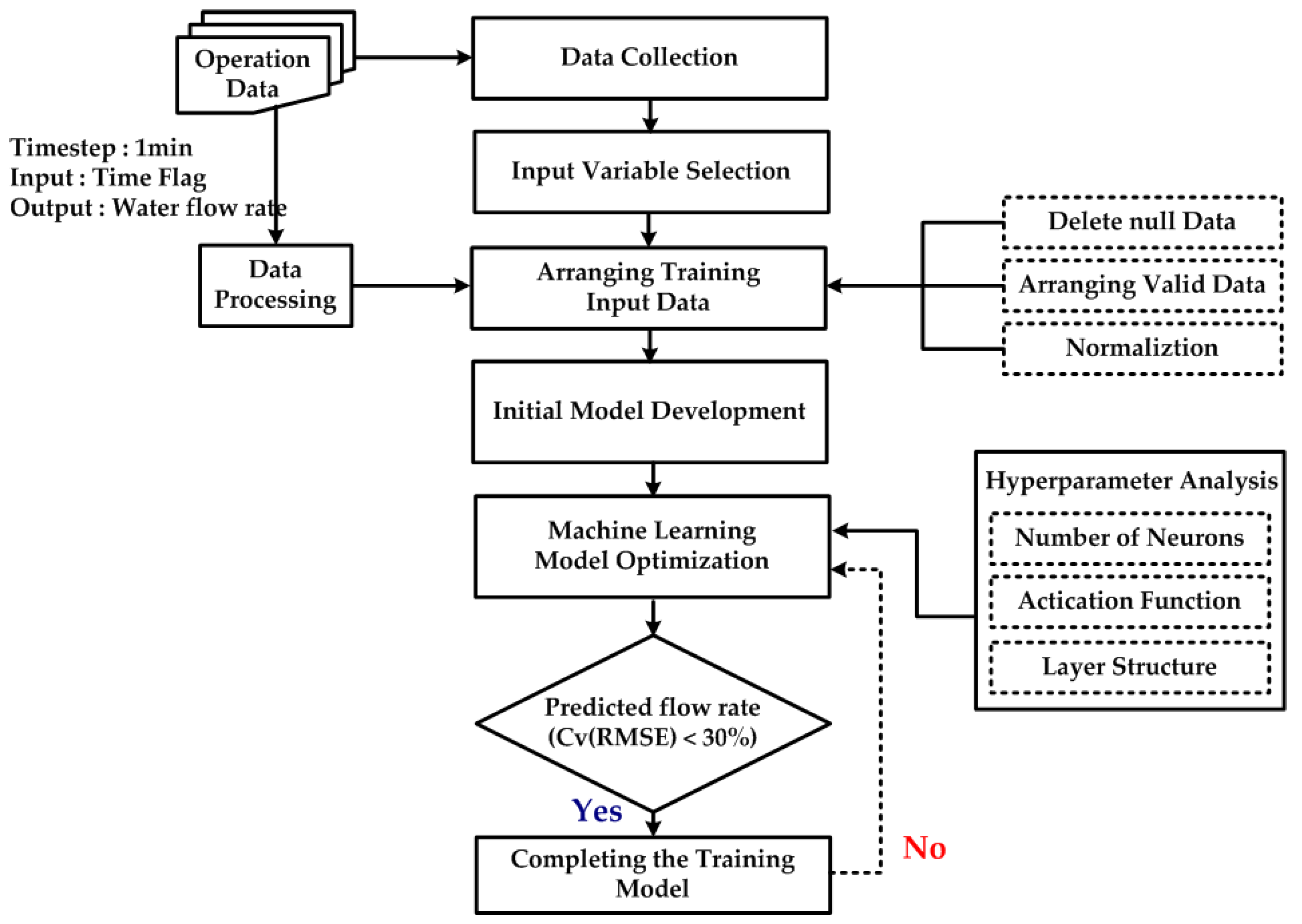
Applsci 13 07771 g002
Figure 3. Process of the development of the performance prediction model.
Applsci 13 07771 g003
Figure 4. Configuration of systems for operational data collection.
Applsci 13 07771 g004
Figure 5. View of systems installed in the target building.
Applsci 13 07771 g005
Figure 6. Equipment for measuring coefficient of performance.
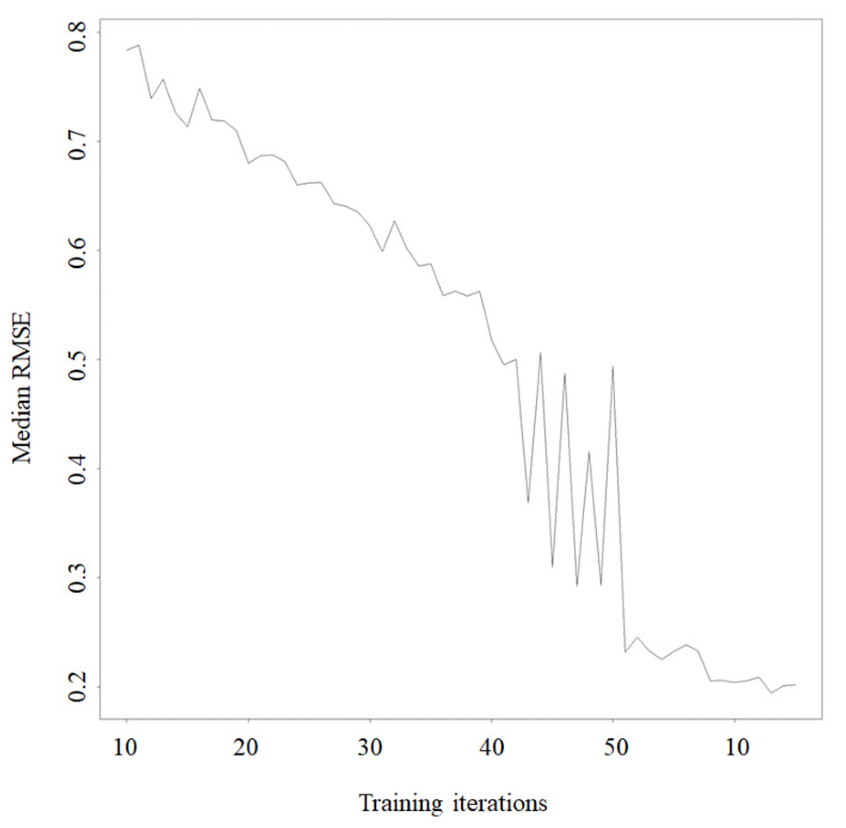
Applsci 13 07771 g006
Figure 7. Prediction model performance analysis for optimizing number of iterations.
Applsci 13 07771 g007
Figure 8. Prediction model performance analysis for hidden layer structure.
Applsci 13 07771 g008
Figure 9. Comparison of prediction performance of prediction model with hyper-parameter optimization.
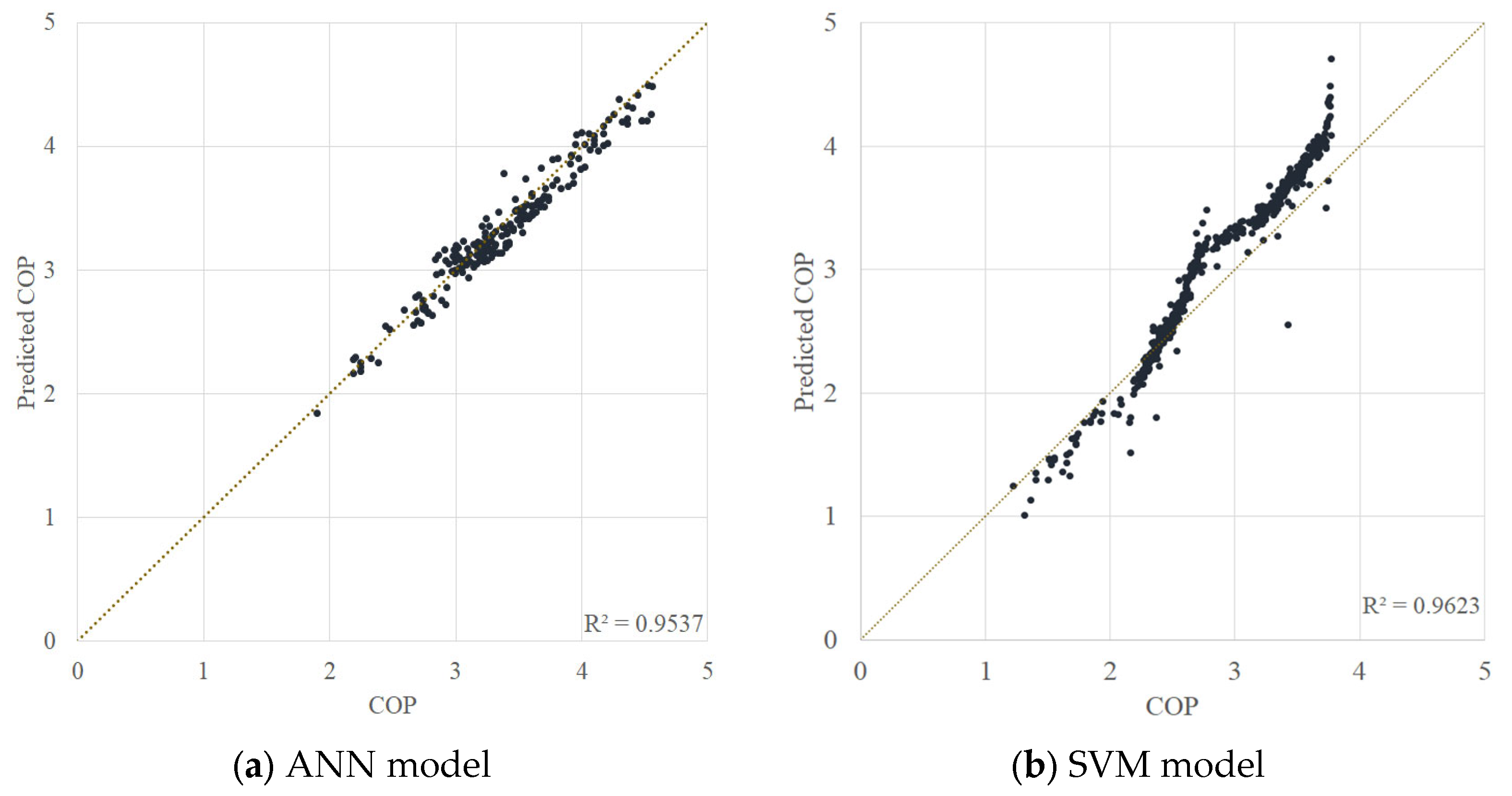
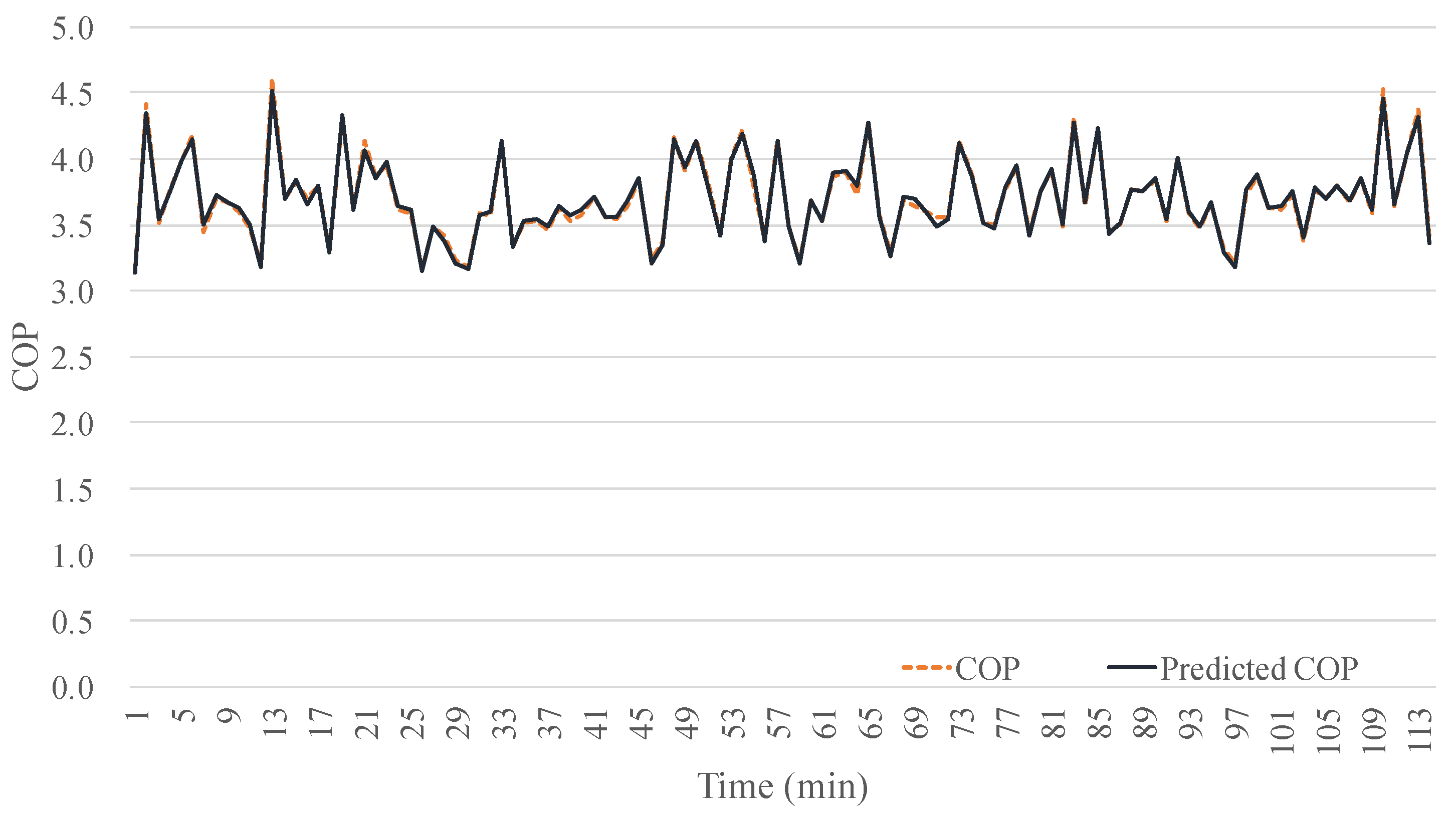
Applsci 13 07771 g009
Figure 10. Comparison of measured performance and prediction performance through an ANN model with optimal hyper-parameter.
Applsci 13 07771 g010
Table 1. Type of hyper-parameter.
Hyper-ParameterContents
Learning rateA variable that determines how fast it will move in the gradient direction
Cost functionA function that estimates the difference between the expected value and the actual value according to the input
Regularization parameterUsing regularization method to avoid and solve overfitting problems
Mini-batch sizeSplitting the entire training data to perform a batch set
Training loopVariables that determine early termination of learning
Hidden unitLearning Optimization Determinants on Training Data
Weight initializationA determinant of performance
Table 2. Previous studies of performance prediction.
CategoryMethodsInputAuthor
Mathematical methodPolynomial7 point (Heating load, etc.)Nam et al.
Machine learningRandom Forest9 point (Power consumption, etc.)Cho
Recurrent Neural Networks12 point (Environmental variable, etc.)Sun et al.
ANN5 point (Power consumption, etc.)Benli
SVM8 points (Heating capacity, etc.)Esen et al.
Adaptive neuro fuzzy inference system8 points (Heating capacity, etc.)Kecman
ANN7 point (Power consumption, etc.)Yilmaz
K-NN8 points (Water flow rate, etc.)Akhlaghi
Random Forest12 point (Power consumption, etc.)Swider
ANN29 point (Power consumption, etc.)Park et al.
ANN5 point (Ground temperature, etc)Esen et al.
ANN3 point (Ground temperature, etc)Esen et al.
Back-propagation Neural Network23 point (Water flow rate, etc)Yan et al.
Random Forest and Back propagation Neural Network16 point (Power consumption, etc.)Lu et al.
Table 3. Overview of buildings for geothermal system operation data collection.
CategoryContents
BuildingUseOffice
Total floor area21,492 m2
SizeB1/F9
Geothermal systemTypeVertical closed-loop
EA7
Capacity (Cooling)105.6 kW
Capacity (Heating)101.4 kW
Number of borehole70
Interval of borehole5 m
Period of data collection2014.02.05~2019.08.31
Table 4. Overview of heat pump systems.
ClassificationCoolingHeating
Capacity (kW)190.61178.93
Power (W)38.0344.52
Flow rate (LPM)600600
COP5.014.02
Table 5. Overview of auxiliary systems.
ClassificationSpec.Contents
Heat source tank18.7 tonCirculation flow rate on heat source side: 5~10 Ton
Load tank18.7 tonCirculation flow rate on load side: 5~100 Ton
Auxiliary heat source10 HPAir-cooled heat pump
Table 6. Overview of operation data collection.
CategoryBuildingTest-Bed
Data collection period1 January 2018~31 December 201825 August 2019~ 27 August 2019
Data collection cycle3 h1 min
Data collection methodBASMeasurement
Temperature range (cooling)24~43 °C20~49 °C
Temperature range (heating)11~24 °C8.1~26.8 °C
Table 7. Accuracy of the measurement devices.
Measurement DeviceSpecific InformationRangesAccuracy
Temperature sensor (°C)RTD (OMEGA)−50~200±0.15%
HOBO U12 (ONSET)−20~70±0.35%
Flow meter (m3/h)FMAG 5000 (SIEMENS)0~400±0.4%
Power meterCW240 (YOKOGAWA)0~3000±0.6%
Table 8. Operation data list.
CategoryUnitSymbol
Outdoor air temperature°C T O A
Source side inlet temperature°C T S , i
Source side outlet temperature°C T S , o
Load side inlet temperature°C T L , i
Load side outlet temperature°C T L , o
Heat pump powerkW W H P
COP- C O P
Pump power kW W P
Table 9. Measurement uncertainty.
CategoryUncertainty (%)
Temperature0.2
Flow rate0.26~0.32
Table 10. Correlation analysis between input data and output data.
Category r r 2
Outdoor air temperature−0.720.52
Source side inlet temperature−0.760.58
Source side outlet temperature0.590.35
Load side inlet temperature0.600.39
Load side outlet temperature0.320.10
Table 11. Statistical analysis of ANN model.
VariablesStatistical Parameters
MeansStandard DeviationMinimumMaximum
COPTraining2.900.711.175.46
Testing2.760.551.223.77
Load side inlet temperatureTraining17.291.7111.6025.00
Testing17.301.7512.1024.20
Load side outlet temperatureTraining16.022.129.0024.40
Testing15.992.169.1023.60
Source side inlet temperatureTraining33.523.8124.2043.50
Testing33.563.7424.6043.00
Source side outlet temperatureTraining37.523.8128.2047.50
Testing37.563.7428.6047.00
Outside temperatureTraining25.432.2122.9033.70
Testing25302.2223.0033.10
Table 12. Statistical analysis of SVM model.
VariablesStatistical Parameters
MeansStandard DeviationMinimumMaximum
COPTraining2.900.711.175.46
Testing2.760.551.223.77
Load side inlet temperatureTraining17.291.7111.6025.00
Testing17.301.7512.1024.20
Load side outlet temperatureTraining16.022.129.0024.40
Testing15.992.169.1023.60
Source side inlet temperatureTraining33.523.8124.2043.50
Testing33.563.7424.6043.00
Source side outlet temperatureTraining37.523.8128.2047.50
Testing37.563.7428.6047.00
Outside temperatureTraining25.432.2122.9033.70
Testing25302.2223.0033.10
Table 13. Structure of initial ANN model.
CategoryContents
FunctionActivationSigmoid
LossMean squared error
Optimization algorithmAdam
Epoch5000
StructureInput layerNumber of layer1
Number of neuron5
Hidden layerNumber of layer1
Number of neuron2
Output layerNumber of layer1
Number of neuron1
Table 14. Structure of initial SVM model.
CategoryContents
TypeEps-regression
KernelPolynomial
Epsilon0.1
Cost1
Gamma1
Table 15. Performance analysis of initial ANN model.
CategoryAccuracy
R2CvRMSEError
ANN0.8917.8−12~11
SVM0.6515.9−14~16
Table 16. Computation time analysis of initial ANN model.
CategoryNormalizationTrain Time
(s)
ANNMin-Max1.43
Standardization0.83
SVMMin-Max2.63
Standardization6.64
Table 17. Hyper-parameter optimization method.
Machine Learning ModelHyper ParameterOptimization Method
ANNTraining iterationsGrid search
Number of hidden layerBayesian optimization
Number of hidden nodeBayesian optimization
SVMKernelGrid search
Number of gammaRandom search
Number of costRandom search
Table 18. Hyper-parameter for optimizing ANN model.
CategoryParameters
ANN1, 2, 3, 4
SVM1~17
Table 19. Hyper-parameter for optimizing SVM model.
CategoryParameters
KernelRadial, Linear, Polynomial, Sigmoid
Cost1, 2, 4, 8, 16
Gamma0.00001, 0.0001, 0.001, 0.01, 0.1, 0
Table 20. Prediction model performance analysis according to hyper-parameter (SVM model 1).
CategoryCost
Gamma124816
0.0000149.647.043.941.439.6
0.000139.338.537.937.736.5
0.00136.534.129.726.524.7
0.0120.412.352.61.7
0.13.24.41.92.42.5
05.23.12.51.20.8
Table 21. Prediction model performance analysis according to hyper-parameter (SVM model 2).
CategoryCost
Gamma124816
0.000012.3342.3342.3132.3102.310
0.00012.3342.3342.3132.3102.310
0.0012.3342.3342.3132.3102.310
0.012.3342.3342.3132.3102.310
0.12.3342.3342.3132.3102.310
02.3342.3342.3132.3102.310
Table 22. Prediction model performance analysis according to hyper-parameter (SVM model 3).
CategoryCost
Gamma124816
0.0000151.2147.0050.0551.0553.05
0.000140.7039.2038.3049.6047.00
0.00150.4749.6948.2246.5044.63
0.0152.9952.9452.8553.0353.02
0.115.3120.8418.3816.3814.95
011.5213.5213.4120.2815.31
Table 23. Prediction model performance analysis according to hyper-parameter (SVM model 1).
CategoryCost
Gamma124816
0.0000151.2149.5547.0043.9241.41
0.000143.0740.7839.2538.4637.89
0.00124.7020.8432.8533.7826.47
0.0138.2737.6536.1246.7253.05
Table 24. Construction of an ANN model with hyper-parameter optimization.
CategoryContents
FunctionActivationSigmoid
LossMean squared error
Optimization algorithmAdam
Epoch5000
StructureInput layerNumber of layer1
Number of neuron4
Hidden layerNumber of layer2
Number of neuron11
Output layerNumber of layer1
Number of neuron1
Table 25. Construction of a SVM model with hyper-parameter optimization.
CategoryContents
TypeEps-regression
KernelRadial
Epsilon16
Cost0
Gamma0.1
Number of support vector1116
Table 26. Performance analysis of prediction model with hyper-parameter optimization.
CategoryAccuracy
MBERMSECvRMSER2
ANN−3.6%15.96%5.4%0.953
SVM−9.8%43.96%8.10%0.962
Disclaimer/Publisher’s Note: The statements, opinions and data contained in all publications are solely those of the individual author(s) and contributor(s) and not of MDPI and/or the editor(s). MDPI and/or the editor(s) disclaim responsibility for any injury to people or property resulting from any ideas, methods, instructions or products referred to in the content.

