Abstract
Compared to the distributed ground-based radar (DGBR), the distributed airborne radar (DAR) has been widely applied due to its stronger anti-damage ability, more degrees of freedom, and better detection view of targets. However, unlike DGBR, the premise for the normal operation of DAR is to maintain stable wireless communication between unmanned aerial vehicles (UAVs). This requires each UAV to make reasonable use of its electromagnetic domain resources. That is, to maximize radar detection performance while ensuring communication performance constraints. However, current research in the field of radar resource allocation has not taken this into account, which greatly limits the practical application of optimization algorithms. Moreover, the current research tends to adopt centralized optimization algorithms. When the baseline of the UAV swarm is long, applying multi-relay methods directly results in heavy communications overhead and long-time delay. Based on the above background, this article aimed to develop a fully distributed algorithm for the joint optimization of radar detection performance and communication transmission performance. This study first took the measurement angle of arrival (AOA) as an example to provide a system model with communication constraints. This model considers the impact of factors such as the UAV location error, UAV communication coverage, and dynamic communication topology of the UAV on joint optimization. A formal representation of the joint optimization is presented. Then, we proposed a joint radar-communication optimization (JRCO) algorithm to fully utilize the electromagnetic domain resources of each UAV. Finally, numerical simulations verified the effectiveness of the proposed JRCO algorithm to traditional radar resource allocation methods.
1. Introduction
In recent years, radars have faced increasingly complex detection environments with the continuous development of target stealth and electronic warfare technology [1,2,3]. Among them, the development of target stealth technology has made the radar cross section (RCS) of targets continuously smaller, making it difficult for traditional radar to detect these targets [4,5]. Meanwhile, the development of electronic warfare technology has led to a rapid increase in the number of various suppression and deception jamming devices [6,7]. This has generated an increasingly crowded spectrum environment faced by traditional radars. Radar must choose appropriate frequency bands to smoothly carry out detection tasks. In this context, the detection ability of traditional single ground-based radar (GBR) further decreases for low-altitude flying targets with a slow velocity [8]. In order to address the aforementioned challenges, the DGBR radar is developing rapidly. Compared to a single radar, DGBR cannot only detect targets from multiple views but also effectively integrate the radars of different frequency bands, polarization modes, and signal bandwidths, achieving a stronger detection performance than a simple combination of single radars [9,10,11]. However, due to the fact that large GBR is always fixed on the ground, the detection view of low-altitude targets is limited. Moreover, due to the fixed location of GBR (i.e., optimal location deployment cannot be achieved), target detection performance is usually limited. In order to overcome these shortcomings, traditional DGBR usually applies methods such as increasing transmission power [12], increasing antenna aperture [13], and increasing signal bandwidth to enhance detection capabilities [14]. However, these methods often lead to a rapid increase in the volume of radar equipment, resulting in the further deterioration of radar maneuverability. Meanwhile, it can lead to serious problems, such as a rapid increase in the overall manufacturing costs of the radar system and difficulties in later maintenance [15].
DAR is a revolutionary technology aimed at traditional DBGR [16,17,18], which is usually of the following advantages: 1. DAR is of more degrees of freedom. DAR can achieve the flexible deployment of radar by flexibly adjusting the locations of the UAVs [19]. This not only enables the more effective detection of targets from multiple angles but also effectively avoids external jamming and attacks [20]. For example, when some nodes in the network are paralyzed by the external jamming of an attack, other UAVs in the network can automatically continue to perform tasks, which greatly improves the robustness of radar networking. 2. DAR is of a better detection view on target. Compared to large DGBRs, DAR typically performs tasks at higher altitudes. High platforms can overcome the weakness of a limited line-of-sight (LOS) of DGBR, making air detection less susceptible to interference from ground clutter and increasing the probability of target detection [21]. 3. DAR is of stronger scalability. Large DGBR can usually only achieve overall system scalability by enhancing the performance (power, antenna aperture, etc.) of each radar in the network, which is easily constrained by the hardware conditions of the radar itself. DAR can flexibly increase or reduce the number of UAVs according to the task requirements [22], making it easier to achieve scalability.
Since DAR is of the above advantages, it has been widely applied in target detection [23], localization [24], tracking [25], recognition [26], imaging [27], and other aspects. The premise for DAR to effectively leverage the above advantages in these tasks is that the radar system can effectively and reasonably allocate its internal resources based on the task requirements. In general, the problem of target localization (or tracking) can be analytically characterized by deriving the Cramer–Rao lower bound (CRLB) for target location estimation, thereby facilitating the construction of an objective function for optimization. At present, most of the current research on distributed radar resource allocation focuses on the joint optimization of multiple parameters within a radar system in the context of localization (or tracking). For example, Zheng Nane’ et al. proposed a joint resource allocation scheme involving the sensor subset, power, and bandwidth. By deriving Bayesian CRLB as the objective function for optimization, the power and bandwidth allocation were both optimized using the convex approximation method of sequence parameters [28]. Shi Chenguang et al. jointly optimized the flight velocity, heading angle, radiation power, signal bandwidth, etc. The proposed method was compared with the following four algorithms: Fixed Path Planning and Optimal Transmit Resource Scheduling, Cooperative Online Path Planning and Transmit Parameter Optimization, Cooperative Online Path Planning and Waveform Parameter Selection, and Online Path Planning and Fixed Transmit Resource Scheduling. The simulation results showed that the algorithm proposed in this article could effectively improve target tracking accuracy while meeting the radio frequency (RF) stealth performance of various airborne radars [29]. In the context of distributed radar localization, Weiwei Zhang et al. jointly optimized the power allocation, bandwidth allocation, and radar node selection in the context of distributed radar localization [30]. Haowei Zhang et al. proposed a joint subarray selection and power allocation (JSSPA) policy for large-scale distributed MIMO radar networks when tracking multiple targets in cluttered environments. Based on the information of the recursive tracking method, optimal resource allocation could be achieved, aiming to improve tracking accuracy [31].
From the above research status, it can be concluded that the current research on distributed radar resource allocation is usually characterized by the following features: 1. The optimization objective is usually the CRLB of the estimated target location. 2. The main optimization variables are electromagnetic parameters and geographic parameters in the radar domain. The electromagnetic parameters here refer to parameters such as the radar power, waveform, bandwidth, etc., while geographic parameters mainly refer to the location of UAVs. However, these methods for distributed radar resource allocation may incur significant problems when directly applied to airborne radar platforms. The biggest difference between DAR and DGBR is that DAR achieves information transmission and instruction distribution through wireless communication, and stable wireless communication is the prerequisite and foundation for airborne radar to perform tasks. In this context, UAVs need to maximize radar detection performance while meeting system communication performance constraints. As radar and communication resources both belong to the electromagnetic domain, the joint planning of radar and communication systems is a significant research field. The current research rarely involves this field, which means that the effective planning and utilization of electromagnetic domain resources in airborne radar systems have not been achieved. This may result in the loss of radar detection performance or the failure of the UAV swarm to fully meet communication performance constraints during the whole process of mission execution.
Currently, very few research studies, represented by Sheng Xu et al. from the University of South Australia, have considered communication constraints in DAR localization systems. For example, they modeled the communication range as an area surrounded by a circle that is centered around the UAV itself [31,32,33]. When the UAV communicates with other UAVs, they fuse the target location information received by the UAV. Nevertheless, these studies only consider the impact of communication performance on information fusion without the collaborative optimization of joint radar-communication electromagnetic domain resources.
Given the above research background, this article focuses on the JRCO algorithm in the context of the passive localization of targets by DAR. A fully distributed JRCO algorithm was proposed to achieve optimal localization performance under communication performance constraints. Compared with traditional methods, The proposed method could significantly improve the target localization performance of the UAV swarm.
The main contributions of this article are as follows:
- A target localization system model for DAR is proposed. Compared with traditional DAR system models, the proposed system model focuses on considering the impact of UAV communications coverage on radar detection performance, the impact of UAV communications coverage on the topology of the UAV communication system, and the impact of the UAV location error on target localization performance.
- A fully distributed JRCO algorithm is proposed. The main idea of this distributed algorithm is to enable each UAV to simultaneously sense the information broadcasted by neighboring UAVs in each time slot and make decisions simultaneously, enabling the joint optimization of radar and communication system parameters, fully utilizing the electromagnetic domain’s freedom. Meanwhile, compared to centralized algorithms, distributed algorithms can continue to perform tasks in the event of a few node failures, avoiding the extreme situation of system paralysis caused by a few key node failures.
- Compared with the current research of Sheng Xu et al., numerical simulations have demonstrated that the proposed algorithm can achieve better target localization performance under communication constraints.
The article was organized as follows: Section 2 introduces the DAR system model under a passive localization background. Section 3 proposes a fully distributed JRCO algorithm and explains the details of each model. Section 4 proves the effectiveness of the proposed algorithm compared to traditional radar domain resource allocation methods through numerical simulations. Section 5 summarizes the entire work and provides prospects for research in the future.
2. System Model
This section first provides a visual description of the scenario, and the specific mathematical modeling is explained in the subsections.
As shown in Figure 1, the passive localization model of an active target by UAV swarms was considered. Each UAV in the swarm performed AOA measurements on the target in each time slot. Each UAV carried radar and communication equipment, where the radar was applied to measure the AOA of the target. The communication equipment was applied to broadcast the information obtained to its neighboring UAVs (specific information will be explained in Section 3.3). In each time slot, each UAV needed to plan the power of the radar system, the power of the communication system, and motion based on the information it sensed (i.e., the information broadcasted by the communication system). The ultimate goal of JRCO was to maximize the accuracy of target localization. In the initial state, all the UAVs departed from the departure area. When the iteration of the JRCO algorithm terminated, all UAVs returned to the departure area and fused all obtained AOA information in the base station.
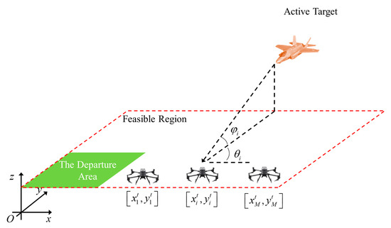
Figure 1.
Scenario of AOA measurement for UAV swarm.
In this context, this article designed a fully distributed JRCO method to maximize the accuracy of target location estimation (Namely the CRLB, which will be derived in Section 2.6). “Distributed” refers to each UAV making independent decisions based on its sensed information at each time slot without being commanded by any other UAV. The reason for considering distributed algorithms instead of centralized algorithms is that when there are a large number of UAVs, centralized algorithms rely on multiple relays for command distribution, which can cause significant communication delays and load.
2.1. The Model of UAV Location
As shown in Figure 1, there were a total of UAVs in the system, and the algorithm executed time slots in total. The meaning of is the maximum time allowed for UAVs to stay in the air. This indicator was set because the UAV swarm executed tasks far away from the base station. The UAV swarm then returns to the base station to unload data only after the task is complete. Therefore, restrictions must be implemented for to prevent the energy depletion of UAVs.
For the safety of the UAV itself, the motion of the UAV swarm is restricted within a rectangular area composed of four vertices: , , , and . This area is defined as a feasible region, as shown in Figure 1. The location coordinate of the -th UAV in the -th time slot can be defined as , and the location state vector of all UAVs is:
The location of the target was defined as . Considering that the location of UAVs might be affected by force majeure, such as wind, the vector composed of the locations of all UAVs in the -th time slot could be represented as:
where , represent the mean vector and location error, which can be represented as:
where , .
All , , and are independent and identically distributed (I.I.D.) Gaussian random variables had a zero mean and variance . The covariance matrix of could be obtained as:
2.2. The Model of UAV Communication Coverage
In order to facilitate the information fusion between each UAV and its neighboring UAVs, each UAV needed to broadcast its own sensed information. These specific types of information sensed are introduced in Section 3.3. Due to the limited payload of each UAV, the communication coverage of each UAV was usually limited. The effective communication coverage of each UAV was an area enclosed by a circle of a certain radius centered around itself. This radius could be defined as the communication coverage radius. The communication coverage radius of the -th UAV in the -th time slot could be defined as , and the state vector of the communication coverage radius of all UAVs in the -th time slot could be defined as ; then:
Obviously, the larger the communication radius, the greater the communication power required by the UAV. For the convenience of subsequent representation, all values of were obtained from a discrete value set, which formed a vector:
2.3. The Definition of UAV Dynamic Communication Topology
The location state vector and the state vector of the communication coverage radius determined the communication connectivity of the whole UAV swarm. The communication connectivity of the UAV swarm was similar to that in graph theory. Taking a directed graph as an example, when -th UAV could sense -th UAV, it was believed that there was a directed path from the -th UAV to the -th UAV. When the communication topology of the UAV swarm was non-connected topology, strongly connected topology, and completely-connected topology, respectively, they corresponded to the concepts of the non-connected graph, strongly connected graph, and completely-connected graph in graph theory, respectively. For more basic concepts of graph theory, please refer to [34].
2.4. The Model of Radar Power and Communication Power
The radar detection power of the -th UAV in the -th time slot could be defined as , and the communication transmission power defined as . In each time slot, the sum of radar, the detection power, and communication transmission power of each UAV was a fixed value, i.e., . was defined as the electromagnetic domain of power.
2.5. The Model of AOA Measurement
For the -th UAV, when it sensed the information broadcasted by the neighboring UAVs (specific information will be introduced in Section 3.3, UAVs including the -th UAV itself), the -th UAV could fuse the information broadcasted by UAVs and obtain an estimation of the target location. It should be noted that the focus of this article was not on target localization algorithms. However, Section 3 used the CRLB of the estimated target location as the objective function to achieve the joint optimization of each UAV location and electromagnetic domain power. The calculation of CRLB required the target location to be known; therefore, it was necessary to estimate the target location before executing the joint optimization algorithm. The AOA measurement based on multiple UAVs was the foundation of target location estimation; therefore, it is necessary to model the measurement process of the AOA first. The specific target location estimation method is provided in Section 3.4. We first provided a measurement model for azimuth AOA.
The azimuth AOA measurement model for the -th UAV in the -th time slot was:
where is the azimuth AOA measurement vector of the neighboring UAVs sensed by the -th UAV in the -th time slot. is the mean vector of the azimuth AOA measured by UAVs around the -th UAV in the -th time slot (the -th UAV cannot sense this value). The measurement error carried by the -th UAV in the -th time slot was . The elements of and could be represented as:
where represents the measured AOA of the neighboring -th UAV sensed by the -th UAV in the -th time slot, and . represents the mean azimuth AOA of the -th UAV sensed by the -th UAV in the -th time slot.
Based on geometric relationships, could be represented as:
where and represent the and coordinates of the surrounding -th UAV sensed by -th UAV in the -th time slot, respectively.
Each element in is an independent zero-mean Gaussian random variable, while the elements in could be represented as:
where represents the AOA measurement error of the neighboring -th UAV sensed by the -th UAV in the -th time slot.
The variance of was . , which represented the azimuth AOA measurement accuracy of the UAV system. The covariance matrix of was:
where represents a diagonal matrix with the dimension .
Equations (12) and (13) describe the azimuth AOA measurement error of the neighboring UAVs from the perspective of the -th UAV. At this point, it was also necessary to describe the azimuth AOA measurement error of all UAVs. From the global perspective of the UAV system, the azimuth AOA measurement error of the -th UAV in the -th time slot in the swarm could be defined as . If represented the state vector composed of the azimuth AOA measurement errors of all UAVs in the -th time slot, there was:
The covariance matrix of was:
The measurement model of elevation AOA was similar to the above content, and in order to avoid repetition, the definitions of , , , , , were not repeated. Meanwhile, in order to simplify the problem appropriately and reasonably, it was believed that held for . Each UAV was of the same measurement error for the elevation and azimuth AOA in a time slot.
2.6. Derivation of CRLB for Target Position Estimation under AOA Model
The ultimate goal of the JRCO algorithm was to achieve a more accurate estimation of the target location by fully utilizing the degrees of freedom in radar-communication systems. Under this condition, it was necessary to theoretically derive the CRLB for target position estimation under the AOA mode. This CRLB would be the objective function for JRCO.
At this point, the measurement model of the radar system was:
Among them, , , , and could represent the measurement vector, measurement function, target state vector, and noise vector, respectively. could be either an echo signal or a measurement value of the parameters, such as the bistatic range. is the true value of the target location, which could be represented by in two-dimensional space.
The elements in Equation (16) are:
where . The covariance matrix corresponding to is .
The elements in the Fisher information matrix of could be calculated based on the following equation [35]:
where represents the trace of the matrix and represents the -th variable in .
The CRLB matrix was:
This article uses the trace of as a quantitative standard for the performance of target localization. At this point, is a matrix. Due to the complexity of deriving the elements in and finding the inverse of , the numerical value of the trace could be directly calculated as the optimization objective function in subsequent algorithms. The process of optimizing the objective function to obtain a gradient could be achieved using mature convex approximation methods such as successive convex approximation (SCA), which is not repeated here.
2.7. The Relationship between and
Obviously, in the -th time slot, the radar detection power and communication transmission power of each UAV satisfied . Due to the impact of the radar detection power on the variance of the AOA measurement error and the impact of the communication transmission power on the communication coverage radius , it was necessary to establish a quantitative relationship between and .
The relationship between and of the -th UAV in the -th time slot was:
Among them, and represent parameters relating to the power consumption of radar systems and communication systems, respectively. The magnitude of these two values could be fitted in practical applications by measuring the power consumption of hardware systems.
2.8. Formal Representation of JRCO
The state of the UAV swarm in time slot could be represented by vector :
The formal representation of JRCO at the -th time slot:
where is the optimization objective function, which is the CRLB of the target location estimation for all UAVs in the swarm. This function could be calculated based on the trace of . , which refers to the Euclidean distance that the -th UAV moves from the -th time slot to the -th time slot. Due to the limitations of the UAV payload, the maximum motion distance of each UAV in each time slot was limited and could not exceed .
It can be noted that the parameters , , , in Equation (24) were based on information obtained from a global perspective (namely, this information was obtained by all the UAVs in the swarm). For a single UAV, it could only sense the information broadcasted by its neighboring UAVs. Therefore, directly adopting the optimization form in Equation (24) would be unrealistic.
If is used to represent the set of UAV locations sensed by the current -th UAV in the -th time slot (including the current UAV itself), the elements in could be represented as:
where .
From the perspective of the -th UAV in the -th time slot, the JRCO could be decomposed into:
where represents the objective function of the -th UAV for optimization.
It should be noted that the optimization problem shown in Equation (26) was executed simultaneously for all the UAVs in each time slot. All UAVs sensed the information and made decisions simultaneously.
Section 4 demonstrates the numerical results that solved the optimization problem shown in Equation (26) through distributed algorithms that could ultimately achieve the sub-optimal solution of the optimization problem shown in Equation (24).
3. JRCO Algorithm
The relationship between the various modules of the JRCO Algorithm is shown in Figure 2. This section elaborates on the logical relationships between the various modules described in Figure 2 first and the overall process of the algorithm. A detailed analysis and description of the functions of each module are presented later in this section. Unless otherwise specified in this section, let , , .
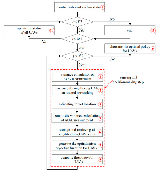
Figure 2.
The flow chart of the JRCO algorithm.
The overall process description of the optimization algorithm was as follows:
Step 1: Before the JRCO algorithm starts iteration, the system state should be initialized, including the locations of each UAV, the communication coverage radius of each UAV, and the location error variance of each UAV. This step corresponds to Box 1 in Figure 2. Next, the algorithm generates policies for all UAVs simultaneously at each time slot , and the process of generating the policies involves traversing all possible values of . When the values of , , and are determined, the current -th UAV begins to enter the following sensing and decision-making steps.
Step 2: In this step, the -th UAV calculates the variance of the AOA measurement error itself based on the communication coverage radius selected for the current -th time slot. This step corresponds to Box 2 in Figure 2.
Step 3: The -th UAV achieves a target location estimation by networking with its neighboring UAVs. These UAVs broadcast their own AOA measurement results and location information to the -th UAV. Specific information before this is introduced later in this section. This step corresponds to Box 3 in Figure 2.
Step 4: Based on the location, the variance of AOA measurement errors, and the AOA measurement value of these UAVs, the -th UAV achieved the estimation of the target location. This estimate could be used to generate the objective function. (This link corresponds to Box 4 in Figure 2). This was because the calculation of the CRLB for target location estimation depended on the location of the target itself, and, in this case, the estimated value of the target location could replace the true value of the target location in the CRLB.
Step 5: Due to the location errors of UAVs themselves, in order to calculate the objective function more accurately, the impact of the location errors of each UAV itself was incorporated into the AOA measurement error. The variance of the AOA measurement error at this point was defined as the composite AOA measurement variance. This step corresponds to Box 5 in Figure 2.
Step 6: Since the communication coverage of each UAV is limited and the UAV needs to achieve optimal deployment through motion, a decision-making mechanism needs to be constructed when the UAV cannot sense any information broadcast by its neighboring UAVs (This state is defined as the current UAV in a disconnected state). When the UAV is not in a disconnected state during a certain time slot, it stores information about itself and the neighboring UAVs in its own memory (The specific types of information are introduced in the second half of this section). When the UAV is in a disconnected state in a certain time slot, the UAV calls the latest networking information in its memory. This link corresponds to Box 6 in Figure 2.
Step 7: With the guarantee of all the above steps, all UAVs can fully construct an objective function. This link corresponds to Box 7 in Figure 2.
Step 8: The -th UAV generates the current activity based on a random projection gradient descent (RPGD) method under the given and . That is, a policy that adjusts and . This step corresponds to Box 8 in Figure 2.
Step 9: When , the -th UAV in the -th time slot has completed all possible attempts at a communication coverage radius. Based on the estimated CRLB corresponding to each communication coverage range for the -th UAV, the optimal policy (including the selection of communication coverage range and motion) for the -th UAV can be determined.
Step 10: When , all UAVs in the -th time slot complete the selection of an optimal policy. At this point, the states of all UAVs are updated simultaneously, and the system enters the time slot.
Step 11: When , the JRCO algorithm terminates. At this point, the UAV swarm returns to the departure area and transmits the AOA measurement information of the -th time slot to the base station in this area.
3.1. Initialization of System State
This module initializes the system state when . Based on the definition of the system state in Equation (23), it is necessary to specify values for , , and . For simplicity, all values in can be made equal, i.e., . represents the initial value of the communication coverage range for all UAVs. Regarding , it is believed that when , all UAVs are distributed in a two-dimensional departure area with a side length of . For , , and follows a uniform-distribution on the interval . The value in can be specified based on the actual scenario of the UAV.
3.2. Variance Calculation of AOA Measurement
The function of this module was to determine the AOA measurement variance of the UAV based on the selected by the -th UAV in the -th time slot when , , and were all determined. The relationship between these two parameters is already shown in Equation (22).
3.3. Sensing of Neighboring UAV States and Networking
The function of this module was to sense the state of neighboring UAVs based on the selected when , , and were all determined. The information sensed by the -th UAV included the and of UAVs around it. To construct the objective function for the current -th UAV, the -th UAV also needed to estimate the target location based on the surrounding UAVs. Therefore, the -th UAV also needed to measure the AOA with neighboring UAVs, and the measurement model is given in Equation (8). The estimation method for the target location is provided in Section 3.4.
3.4. Estimating Target Location
Based on the measurement model given in Equation (8) and the AOA measurement values of neighboring UAVs, this subsection designed relevant parameter estimation algorithms to estimate the target location. In each time slot, each UAV could only construct an objective function based on Equation (21) by estimating the target location. At present, most of the current research on optimizing the CRLB [36,37,38,39] has assumed that the accurate target location is known. It is obviously unreasonable that the target location is known before the UAV swarm can obtain an accurate target location estimation.
In the case of neighboring UAVs forming a network together and, based on the geometric relationship between each UAV and the target, there was:
Tan operations can be performed on both sides simultaneously and multiplied by to obtain:
where .
After some mathematical manipulations, there were:
where:
When the variance of AOA measurement errors for each UAV was relatively small, the following approximate relationship held:
Thus, the following pseudo-linear equation could be obtained:
where:
Due to , Equation (36) corresponded to equations, namely:
where:
The above process was repeated and we obtained:
where:
Defining , and . represented the vector of the location parameter, and Equations (40) and (44) could be solved using methods such as weighted least squares (WLS). If , then after some mathematical manipulation, the covariance matrix of could be obtained as:
After some further mathematical manipulation, the cost function of the WLS method could be obtained:
where was the estimated value of . The cost function could be minimized to obtain . The solving process of WLS need not be elaborated here.
3.5. Composite Variance Calculation of AOA Measurement
At present, all input variables for constructing the objective function of -th UAV in the -th time slot could be obtained, namely , , and . According to Equation (21), the objective function could be constructed at this time. However, did not include the impact of the UAV location error on AOA measurement at this time.
This section considers the impact of the UAV location error on the AOA measurement based on the covariance matrix . For a local networking system composed of UAVs around the -th UAV, the errors in the , and coordinates of each UAV could be defined as , and respectively, and the AOA measurement error was . Thus, they were all Gaussian random variables with a zero mean, i.e., , , and
. For the theoretical basis of Gaussian random variables for the above random variables, please refer to the literature [40].
The AOA estimation error caused by the location error of the -th UAV in the local networking system of -th UAV could be defined as . At this point, the azimuth AOA measurement error could be determined by , and the elevation AOA measurement error could be determined by . Based on the geometric relationship, there were:
The derivation of PDFs for and was not an easy process, but numerical simulations could verify that and approximately followed Gaussian distributions. The PDF based on sample fitting and Gaussian distribution fitting was verified under the condition of , , , (shown in Figure 3). The locations of the sensor are all , in Figure 3. Based on the properties of the Gaussian distribution, it could be concluded that both and follow the Gaussian distribution at this time. Their variances were defined as and , and their corresponding Covariance matrix was defined as and , respectively.
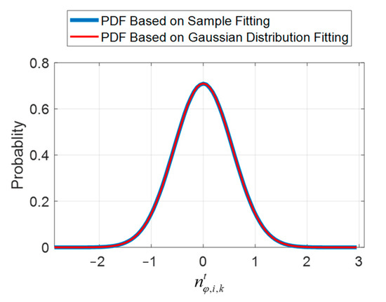
Figure 3.
Approximated PDF for .
.
3.6. Storage and Retrieving of Neighboring UAV State
As mentioned earlier, in order to ensure that each UAV could smoothly construct an objective function in a disconnected state, each UAV needed to store and retrieve the state of the neighboring UAVs. The process was as follows: when the -th UAV was not in a disconnected state in the -th time slot, the -th UAV needed to temporarily store , , and at this time. Once the -th UAV was in a disconnected state in the -th time slot, the -th UAV could continue to complete the construction of the objective function by calling the information of , , and in the -th time slot. Each UAV stored and retrieved information independently. If the UAV was not in a disconnected state in two consecutive time slots (such as the -th and -th time slots), the stored information in the -th time slot could delete the information in the -th time slot to save memory.
The vector corresponding to the storage information of the -th UAV location in the -th time slot could be defined as:
where .
The vector corresponding to the storage information of the composite measurement variance of AOA in the -th time slot could be defined as:
The vector corresponding to the storage information of the target location estimation in the -th time slot was defined as:
Even if the -th UAV could not sense any state information shared by other UAVs within a certain time slot, it could still smoothly generate optimization objectives based on the rules above.
3.7. Generate the Optimization Objective Function
So far, the -th UAV was of the ability to build optimization objectives based on the information of the neighboring UAVs (or its own stored information). Based on Equation (21), when , , , were known, the CRLB of the target location estimation was also known.
3.8. Generate the Policy for the -th UAV
For the optimization objective function of the -th UAV in the -th time slot, the method based on a random projection gradient descent (RPGD) could be applied to optimize the location of the UAV. The pseudocode of the algorithm is shown in Algorithm 1.
| Algorithm 1. RPGD algorithm for the -th UAV in the -th time slot. | |
| 01 | Initialize , , , , |
| 02 | Let |
| 03 | for |
| 04 | Randomly sampling on a unit sphere |
| 05 | |
| 06 | |
| 07 | end for |
| 08 | |
| 09 | Return |
and in Algorithm 1 represent the maximum step size and tolerance in the RPGD method, respectively. and represent the iteration variable and iteration number, respectively. is determined by , where is the step size of each iteration, which can be determined by . is the maximum step size of the motion within a time slot.
When the UAV is in a disconnected state, it can adopt the following three policies. To balance these three motion policies, and can be defined. When for the -th UAV, the system randomly generated a uniformly distributed random number between 0 and 1. At this point, the -th UAV generated the next location policy based on the size of in the following three methods:
Method 1: When , the -th UAV generated based on the algorithm shown in Table I.
Method 2: When , the -th UAV moved by in the direction of the geometric mean of the stored information of the location;
Method 3: When , the UAV moved by in a random direction (with a uniform distribution at intervals ).
3.9. Pseudocode of JRCO Algorithm
The pseudocode of the JRCO algorithm is shown in Algorithm 2.
| Algorithm 2. The pseudocode of the JRCO algorithm. | |
| 01 | Initialize , , |
| 02 | for |
| 03 | for |
| 04 | for |
| 05 | calculate based on |
| 06 | get , , from neighboring UAVs |
| 07 | estimate the position of the target based on and |
| 08 | get , , based on , , , , and Monte Carlo method |
| 09 | if |
| 10 | update the memory in , and |
| 11 | else |
| 12 | retrieve the memory from , and |
| 13 | end if |
| 14 | get the objective function |
| 15 | get the optimal policy for the -th UAV based on current |
| 16 | end for |
| 17 | select the optimal coverage radius and optimal for the -th UAV |
| 18 | end for |
| 19 | update and for all UAVs |
| 20 | end for |
4. Numerical Results
This section validates the effectiveness of the proposed JRCO algorithm through a numerical simulation. This section consists of one experimental group and four control groups. The MSE curves of the target location estimation were plotted separately. All numerical simulation results in this section were run on a processor 11th Gen Intel(R) Core(TM) i7-11800H @ 2.30 GHz, using the numerical simulation tool MATLAB R2020a.
4.1. The First Set of Parameters
The simulation parameters of the experimental group are shown in Table 1. The focus of parameter selection was mainly on the geometric scale between the UAV and the target. The selection of parameters was mainly based on the currently distributed radar literature, and the literature selected for this subsection was [41].

Table 1.
The first set of parameters for numerical simulation.
The meanings of the experimental group and the four control groups were as follows:
Experimental group: Under the simulation parameters shown in Table 1, the joint optimization method in Algorithm 2 was applied.
Control group 1 (Sheng Xu’s method [31,32,33]): Based on the simulation parameters shown in Table 1 and the JRCO algorithm in Algorithm 2, the communication coverage range of each UAV was kept unchanged (set at 150 m), and this control algorithm only planned the location of each UAV. At this point, the radar detection power and communication transmission power of each UAV remained unchanged with time, and the other conditions remained consistent with the experimental group. At this point, the optimization method only took the estimated CRLB as the optimization objective and planned the location (or path) of the UAV. This method was the same as the method in references [31,32,33]; therefore, the control group aimed to compare the proposed JRCO algorithm with the current research of Sheng Xu et al.
Control group 2: Under the simulation parameters shown in Table 1, the JRCO algorithm in Algorithm 2 was performed, but the communication coverage range of all UAVs was infinite. The measurement error of AOA for each UAV was calculated based on the communication coverage radius of 150 m, which was equivalent to a centralized algorithm. Meanwhile, the optimal locations of all UAVs were generated through the same RPGD method. That is, all UAVs applied an equal step size in the RPGD method when executing the algorithm, and other conditions were consistent with the experimental group.
Control group 3: Under the simulation parameters shown in Table 1 and based on the JRCO algorithm in Algorithm 2, the communication coverage range of all UAVs was infinite. The measurement error of the AOA for each UAV was calculated based on a communication coverage radius of 150 m, which was equivalent to a centralized algorithm. However, the location of only one UAV was planned in each time slot, and all UAVs were planned in a sequence of a different time slot, while the other conditions were consistent with the experimental group.
Control group 4: Under the simulation parameters shown in Table 1, the JRCO algorithm in Algorithm 2 was performed, but the communication coverage range of all UAVs was infinite. The measurement error of AOA for each UAV was calculated based on the communication coverage radius of 150 m, which was equivalent to a centralized algorithm. Other conditions were consistent with the experimental group.
Figure 4a shows the trend of MSE for the target location estimation when the time slot range was 0–100. It can be seen that at the beginning of the iteration, the MSE curves corresponding to the experimental group, control group 1, and control group 4 decreased significantly faster than the MSE curves corresponding to the control group 2 and control group 3.
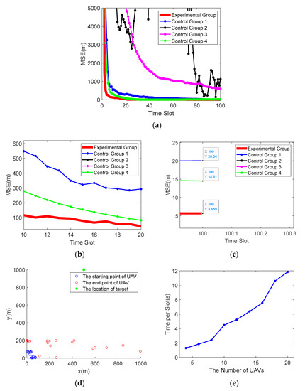
Figure 4.
MSE versus time slot under the first set of parameters. (a) MSE when the time slot range was taken as 0–100. (b) MSE when the time slot range was taken as 10–20. (c) MSE when the time slot range was taken as 100. (d) The initial and final locations of UAVs. (e) The relationship between the time consumption per time slot of the JRCO algorithm and the number of UAVs.
Based on Figure 4b, it can be seen that, at the beginning of the iteration, the experimental group showed better performance than control group 1 (Sheng Xu’s method [31,33]): For example, in the 10th time slot, the MSE generated by the experimental group was about 440 m lower than that of control group 1. In the 20th time slot, the MSE generated by the experimental group was approximately 270 m lower than that of control group 1. This fully proved the effectiveness of the JRCO algorithm, which achieved a better performance in target localization than the current research of Sheng Xu et al. The JRCO algorithm adopted by the experimental group achieved a good target localization performance by fully utilizing the degrees of freedom in radar communication systems.
The MSE curves of the experimental group, control group 2, and control group 3 were compared, as shown in Figure 4a. It was obvious that the MSE of the experimental group decreased the fastest overtime at this time slot scale. Control group 2 applied a centralized algorithm, but its corresponding MSE values showed significant fluctuations. This was because the same step size across all the time slots led to the poorer convergence performance of the JRCO algorithm. This resulted in no convergence trend in the curve of control group 2, and the iterative efficiency of the algorithm in this group was relatively low. Although control group 3 also adopted a centralized algorithm, the location of only one UAV was optimized in each time slot. This greatly reduced the iterative efficiency of the algorithm.
Finally, the MSE curves corresponding to the experimental group and control group 4 were compared. It could be concluded that these three curves were relatively close on the scale of 0–100 time slots. Therefore, Figure 4b,c provide the MSE curves in the range of 10–20 time slots and the 100th time slot, respectively. From the condition settings of the five simulation experiments, it could be seen that the optimization algorithm applied in control group 4 could provide the best performance (i.e., the corresponding MSE curve decreased the fastest over time). For Figure 4c, it could be seen that at the end of the algorithm, the MSE curves of control group 4 and control group 1 were actually closer, and the experimental group obtained the lowest MSE. The MSE of the experimental group (5.66 m) decreased by approximately 60.99% (8.85 m) compared to the MSE of the control group 4 (14.51 m). This fully demonstrated the potential and advantages of the proposed JRCO algorithm.
To demonstrate other details generated by the joint optimization algorithm, Figure 4d provides the initial and final locations of the UAV swarm. Figure 4e shows the average operation time of each time slot as a function of the number of UAVs (only the results on the two-dimensional plane were plotted).
4.2. The Second Set of Parameters
The simulation parameters of the experimental group are shown in Table 2. In terms of parameter selection, the literature selected for this subsection was [42]. The parameters not given in Table 2 were consistent with Table 1. The setting method for one experimental group and four control groups was consistent with Section 4.1, with a default communication range of 1.5 km. The corresponding numerical simulation results are shown in Figure 5.
Table 2.
The second set of parameters for numerical simulation.
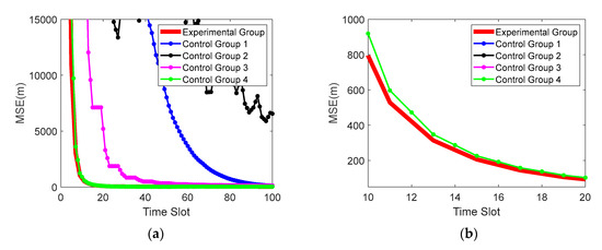
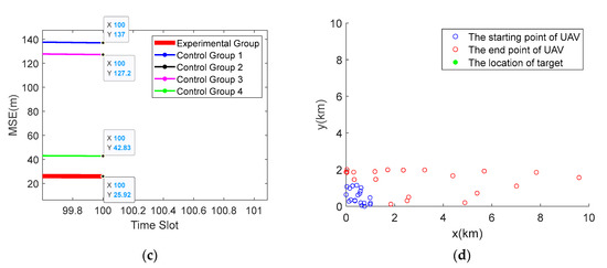
Figure 5.
MSE versus time slot under the second set of parameters. (a) MSE when the time slot range was taken as 0–100. (b) MSE when the time slot range was taken as 10–20. (c) MSE when the time slot range was taken as 100. (d) The initial and final locations of UAVs.
Figure 5a shows the MSE curves generated by each group when the time slot range was 0–100. Obviously, at this time, the curves corresponding to the experimental group, control group 3, and control group 4 decreased rapidly. Figure 5b shows a comparison of the curves between the experimental group and the control group 4 when the time slot was 10–20. It can be seen that in the early stages of algorithm iteration, the experimental group showed a better performance than any control group. Figure 5c shows the final results of MSE generated by each group for the 100th time slot. At this time, the MSE of the experimental group (25.92 m) decreased by approximately 39.48% (16.91 m) compared to the MSE of control group 4 (42.83 m). The above numerical simulation results fully demonstrate the effectiveness of the proposed JRCO algorithm, and the joint optimization algorithm was suitable for a wide range of scenarios. Figure 5d shows the initial and final locations of the UAV swarm.
5. Conclusions and Future Works
This article proposes a novel joint optimization algorithm for the radar detection-communication transmission of DAR. Compared with current research on the resource allocation of DAR, the JRCO algorithm is mainly of the following two prominent features: firstly, it synergistically utilizes the degrees of freedom in both the radar system and communication system. It overcomes the limitation of traditional radar resource allocation that only focuses on the optimization variables of radar systems. The proposed JRCO algorithm could achieve a better radar detection performance while ensuring communication performance constraints. The second is that the JRCO algorithm was completely distributed, which was in stark contrast to the current centralized algorithms for resource allocation. Distributed algorithms can enable the system to be of a higher task execution efficiency, lower communication transmission delay, and stronger anti-damage ability.
In order to implement the JRCO algorithm, this article first took the estimation of the target location in the passive AOA measurement mode as an example; this comprehensively modeled the system from various aspects, such as the location error and communication coverage of the UAV and provided a formal representation of the joint optimization problem. Then, the JRCO algorithm was elaborated into eight subsections. Finally, the effectiveness of the JRCO algorithm was verified by a numerical simulation in formal verification that is, the JRCO algorithm could achieve a better target localization performance.
However, the main drawback of the JRCO algorithm was that the iteration and update process was relatively slow. From Figure 4e, it could be seen that as the number of the UAV swarm increased, the iteration efficiency of the JRCO algorithm significantly decreased. In future work, we intend to focus on improving this issue. In addition, more complex radar systems and communication system topologies that are suitable for airborne radar will be considered. For radar systems, it is also possible to optimize the CRLB for target position estimation under active detection background. For communication systems, the presence of relays should be considered.
Author Contributions
Methodology, G.D. and Q.W.; Supervision, Y.H. and J.Y.; Writing—original draft, G.D.; Writing—review and editing, J.Y. and S.W. All authors have read and agreed to the published version of the manuscript.
Funding
This work was supported by the National Natural Science Foundation of China under Grant No. 91948303.
Institutional Review Board Statement
Not applicable.
Informed Consent Statement
Not applicable.
Data Availability Statement
Not applicable.
Conflicts of Interest
The authors declare no conflict of interest.
References
- Zhang, H.; Yu, L.; Chen, Y.; Wei, Y. Fast complex-valued CNN for radar jamming signal recognition. Remote Sens. 2021, 13, 2867. [Google Scholar] [CrossRef]
- Lang, B.; Gong, J. JR-TFViT: A Lightweight Efficient Radar Jamming Recognition Network Based on Global Representation of the Time–Frequency Domain. Electronics 2022, 11, 2794. [Google Scholar] [CrossRef]
- Hou, Y.; Ren, H.; Lv, Q.; Wu, L.; Yang, X.; Quan, Y. Radar-Jamming Classification in the Event of Insufficient Samples Using Transfer Learning. Symmetry 2022, 14, 2318. [Google Scholar] [CrossRef]
- Chen, J.; Zheng, H.; Su, M.; Du, T.; Lin, C.; Ji, S. Invisible poisoning: Highly stealthy targeted poisoning attack. In Proceedings of the Information Security and Cryptology: 15th International Conference, Inscrypt 2019, Nanjing, China, 6–8 December 2019; Revised Selected Papers 15, 2020. pp. 173–198. [Google Scholar]
- Banerjee, P.; Chu, L.; Zhang, Y.; Lakshmanan, L.V.; Wang, L. Stealthy targeted data poisoning attack on knowledge graphs. In Proceedings of the 2021 IEEE 37th International Conference on Data Engineering (ICDE), Chania, Greece, 19–22 April 2021; pp. 2069–2074. [Google Scholar]
- Lv, Q.; Quan, Y.; Feng, W.; Sha, M.; Dong, S.; Xing, M. Radar deception jamming recognition based on weighted ensemble CNN with transfer learning. IEEE Trans. Geosci. Remote Sens. 2021, 60, 5107511. [Google Scholar]
- Tan, M.; Wang, C.; Xue, B.; Xu, J. A novel deceptive jamming approach against frequency diverse array radar. IEEE Sens. J. 2020, 21, 8323–8332. [Google Scholar] [CrossRef]
- Pieraccini, M.; Miccinesi, L. Ground-based radar interferometry: A bibliographic review. Remote Sens. 2019, 11, 1029. [Google Scholar] [CrossRef]
- Yi, W.; Yuan, Y.; Hoseinnezhad, R.; Kong, L. Resource scheduling for distributed multi-target tracking in netted colocated MIMO radar systems. IEEE Trans. Signal Process. 2020, 68, 1602–1617. [Google Scholar] [CrossRef]
- Zhang, H.; Liu, W.; Zhang, Z.; Lu, W.; Xie, J. Joint target assignment and power allocation in multiple distributed MIMO radar networks. IEEE Syst. J. 2020, 15, 694–704. [Google Scholar] [CrossRef]
- Wang, H.; Li, S.; Xue, X.; Xiao, X.; Zheng, X. Distributed coherent microwave photonic radar with a high-precision fiber-optic time and frequency network. Opt. Express 2020, 28, 31241–31252. [Google Scholar] [CrossRef]
- Shi, C.; Ding, L.; Wang, F.; Salous, S.; Zhou, J. Low probability of intercept-based collaborative power and bandwidth allocation strategy for multi-target tracking in distributed radar network system. IEEE Sens. J. 2020, 20, 6367–6377. [Google Scholar] [CrossRef]
- Carrer, L.; Gerekos, C.; Bovolo, F.; Bruzzone, L. Distributed radar sounder: A novel concept for subsurface investigations using sensors in formation flight. IEEE Trans. Geosci. Remote Sens. 2019, 57, 9791–9809. [Google Scholar] [CrossRef]
- Lembo, L.; Ghelfi, P.; Bogoni, A. Antenna position optimization in a MIMO distributed radar network through genetic algorithms. In Proceedings of the 2019 20th International Radar Symposium (IRS), Ulm, Germany, 26–28 June 2019; pp. 1–6. [Google Scholar]
- Wang, S.; Liu, G.; Jing, G.; Feng, Q.; Liu, H.; Guo, Y. State-of-the-art review of ground penetrating radar (GPR) applications for railway ballast inspection. Sensors 2022, 22, 2450. [Google Scholar] [CrossRef] [PubMed]
- Jinming, C.; Tong, W.; Xiaoyu, L.; Jianxin, W. Time and phase synchronization using clutter observations in airborne distributed coherent aperture radars. Chin. J. Aeronaut. 2022, 35, 432–449. [Google Scholar]
- Chen, J.; Wang, T.; Liu, X.; Wu, J.J.I.S.J. Identifiability Analysis of Positioning and Synchronization Errors in Airborne Distributed Coherence Aperture Radars. IEEE Sens. J. 2022, 22, 5978–5993. [Google Scholar] [CrossRef]
- Ding, K.; Wu, F.; Li, S.; Li, B.; He, Y.; Zhang, Y. Design and research on a power distribution system for airborne radar. J. Eng. 2019, 2019, 1528–1531. [Google Scholar] [CrossRef]
- Zhao, H.; Wang, H.; Wu, W.; Wei, J. Deployment algorithms for UAV airborne networks toward on-demand coverage. IEEE J. Sel. Areas Commun. 2018, 36, 2015–2031. [Google Scholar] [CrossRef]
- Miao, Y.; Liu, F.; Liu, H.; Li, H. Clutter Jamming Suppression for Airborne Distributed Coherent Aperture Radar Based on Prior Clutter Subspace Projection. Remote Sens. 2022, 14, 5912. [Google Scholar] [CrossRef]
- Liggins, M.E.; Chong, C.-Y. Distributed multi-platform fusion for enhanced radar management. In Proceedings of the 1997 IEEE National Radar Conference, Syracuse, NY, USA, 13–15 May 1997; pp. 115–119. [Google Scholar]
- Brandfass, M.; Dallinger, A.; Weidmann, K. Modular, scalable multifunction airborne radar systems for high performance ISR applications. In Proceedings of the 2018 19th International Radar Symposium (IRS), Bonn, Germany, 20–22 June 2018; pp. 1–10. [Google Scholar]
- Duk, V.; Wojaczek, P.; Rosenberg, L.; Cristallini, D.; O’Hagan, D.W. Airborne passive radar detection for the APART-GAS trial. In Proceedings of the 2020 IEEE Radar Conference (RadarConf20), Florence, Italy, 21–25 September 2020; pp. 1–6. [Google Scholar]
- Xu, J.; Liao, G.; Zhang, Y.; Ji, H.; Huang, L. An adaptive range-angle-Doppler processing approach for FDA-MIMO radar using three-dimensional localization. IEEE J. Sel. Top. Signal Process. 2016, 11, 309–320. [Google Scholar] [CrossRef]
- Joshi, S.K.; Baumgartner, S.V.; Krieger, G. Tracking and track management of extended targets in range-Doppler using range-compressed airborne radar data. IEEE Trans. Geosci. Remote Sens. 2021, 60, 5102720. [Google Scholar] [CrossRef]
- Wang, W.; Wang, Y. A Parameter-Optimized SLS-TSVM Method for Working Modes Recognition of Airborne Fire Control Radar. In Proceedings of the 2020 IEEE 4th Information Technology, Networking, Electronic and Automation Control Conference (ITNEC), Chongqing, China, 12–14 June 2020; pp. 948–953. [Google Scholar]
- Nenashev, V.; Sentsov, A.; Shepeta, A. Formation of radar image the earth’s surface in the front zone review two-position systems airborne radar. In Proceedings of the 2019 Wave Electronics and its Application in Information and Telecommunication Systems (WECONF), Saint Petersburg, Russia, 3–7 June 2019; pp. 1–5. [Google Scholar]
- Na’e, Z.; Yang, S.; Xiyu, S.; Song, C. Joint resource allocation scheme for target tracking in distributed MIMO radar systems. J. Syst. Eng. Electron. 2019, 30, 709–719. [Google Scholar]
- Yijie, W.; Xiangrong, D. Joint transmit resources and trajectory planning for target tracking in airborne radar networks. J. Radars 2022, 11, 778–793. [Google Scholar]
- Zhang, W.; Shi, C.; Zhou, J. Power Minimization-Based Joint Resource Allocation Algorithm for Target Localization in Noncoherent Distributed MIMO Radar System. IEEE Syst. J. 2021, 16, 2183–2194. [Google Scholar] [CrossRef]
- Xu, S.; Dogançay, K.; Hmam, H. Distributed path optimization of multiple UAVs for AOA target localization. In Proceedings of the 2016 IEEE International Conference on Acoustics, Speech and Signal Processing (ICASSP), Shanghai, China, 20–25 March 2016; pp. 3141–3145. [Google Scholar]
- Xu, S.; Doğançay, K.; Hmam, H. Distributed pseudolinear estimation and UAV path optimization for 3D AOA target tracking. Signal Process. 2017, 133, 64–78. [Google Scholar] [CrossRef]
- Xu, S.; Doğançay, K.; Hmam, H. 3D AOA target tracking using distributed sensors with multi-hop information sharing. Signal Process. 2018, 144, 192–200. [Google Scholar] [CrossRef]
- Tutte, W.T.; Tutte, W.T. Graph Theory; Cambridge University Press: Cambridge, UK, 2001; Volume 21. [Google Scholar]
- Cheng, Y.; Wang, X.; Caelli, T.; Li, X.; Moran, B. On information resolution of radar systems. IEEE Trans. Aerosp. Electron. Syst. 2012, 48, 3084–3102. [Google Scholar] [CrossRef]
- Xu, S.; Doğançay, K. Optimal sensor placement for 3-D angle-of-arrival target localization. IEEE Trans. Aerosp. Electron. Syst. 2017, 53, 1196–1211. [Google Scholar] [CrossRef]
- Xu, S. Optimal sensor placement for target localization using hybrid RSS, AOA and TOA measurements. IEEE Commun. Lett. 2020, 24, 1966–1970. [Google Scholar] [CrossRef]
- Xu, S.; Ou, Y.; Zheng, W. Optimal sensor-target geometries for 3-D static target localization using received-signal-strength measurements. IEEE Signal Process. Lett. 2019, 26, 966–970. [Google Scholar] [CrossRef]
- Xu, S.; Rice, M.; Rice, F. Optimal TOA-sensor placement for two target localization simultaneously using shared sensors. IEEE Commun. Lett. 2021, 25, 2584–2588. [Google Scholar] [CrossRef]
- Dabiri, M.T.; Rezaee, M.; Yazdanian, V.; Maham, B.; Saad, W.; Hong, C. 3D channel characterization and performance analysis of UAV-assisted millimeter wave links. IEEE Trans. Wirel. Commun. 2020, 20, 110–125. [Google Scholar] [CrossRef]
- Du, Y.; Wei, P. An explicit solution for target localization in noncoherent distributed MIMO radar systems. IEEE Signal Process. Lett. 2014, 21, 1093–1097. [Google Scholar]
- Ge, M.; Cui, G.; Shi, Q.; Kong, L.; Li, N. Mainlobe jamming suppression based on joint blind source separation for distributed radar. In Proceedings of the 2019 IEEE Radar Conference (RadarConf), Boston, MA, USA, 22–26 April 2019; pp. 1–5. [Google Scholar]


Disclaimer/Publisher’s Note: The statements, opinions and data contained in all publications are solely those of the individual author(s) and contributor(s) and not of MDPI and/or the editor(s). MDPI and/or the editor(s) disclaim responsibility for any injury to people or property resulting from any ideas, methods, instructions or products referred to in the content. |
© 2023 by the authors. Licensee MDPI, Basel, Switzerland. This article is an open access article distributed under the terms and conditions of the Creative Commons Attribution (CC BY) license (https://creativecommons.org/licenses/by/4.0/).