Identification of the Physical Dependencies of Accurate Oil Level Measurement for Automotive Applications

Abstract

The presented research addresses the problem of dependency analysis of the ultrasonic signal measured by a sensor in an engine oil bath. The dependency analysis is performed on a selected ultrasonic signal sensor solution containing its own generator and an ultrasonic signal receiver detecting the level of the oil in which it is immersed. The influence of the resulting amplitude of the received ultrasonic signal is mainly due to the level of the measured oil level and the oil temperature, as shown by the regression analysis and ANOVA (Analysis of Variance) testing performed. The analyzed dependence of the time determination of the length of the generated ultrasonic signal envelope is given by a set threshold value, which can be dynamically adjusted based on the backtracking evaluation. The analysis results in the form of approximation by the dependency algorithm confirm the assumption of possible standardization of the envelope parameters with the achievement of accuracy up to 99.02%. The analyzed parameters approximated by the temperature and oil level dependence algorithms include the amplitude of the measured signal, steepness of the rising edge, duration of the envelope, and the digitally processed amplitude value.

1. Introduction

In technical practice, precise liquid level measurement is often necessary [1]. One common method for such measurement is the ultrasonic signal measurement, which has various applications beyond level measurement, including determining the composition of multiphase flow of oil, water, and gas in pipelines [2], monitoring pipeline corrosion in oil and gas [3], measuring the three-phase flow of oil, gas, and water in the oil production and transportation process [4], measuring the density of liquids [5,6], and determining the concentration of emulsion liquids [7].

The automotive industry deploys a wide range of sensors and sensor systems in its solutions, and one of the purposes is to measure oil levels. In general, for the purpose of liquid level measurement, for example, ultrasonic [1,8,9,10], optical [11,12,13], or capacitive [14,15,16] principles can be used [17]. However, not all of them are suitable for measuring the oil level as there are constant changes in the oil properties and even the environment of the engine itself [18]. The most commonly used oil level sensors are ultrasonic-based [17] thanks to their lower price and good properties for measuring an oil level. There is pressure from the automotive industry to keep costs as low as possible, but this is not compatible with the high accuracy and quality of the sensors used.

This study focuses specifically on improving the accuracy of oil level measurement with an ultrasonic level sensor that gives measurement range and temperature range, where the design and materials used in the sensor can affect the signal generated and analyzed [19,20]. A major challenge in using ultrasonic signal measurement for oil level measurement is the significant dependence of the ultrasonic signal response on temperature and viscosity [19,21,22,23]) describing physical phenomena and possible elimination-type methods.

Results of measurements of this study are based on an MCU Renesas RL78/F13 processor, which controls the ultrasonic measurement with the implemented algorithm of ultrasonic signal generation and processing, while a comparison of other processors for controlling the measurement processes can be found in a separate study by Shan et al. [24]. Unlike existing and described methods, the novelty of this work lies in the use of statistical methods of ANOVA and regression analysis to improve the accuracy of oil level measurements without changing the hardware configuration. By analyzing and correcting ultrasonic signal measurements, this study provides a precise and computationally validated method of level detection [21].

The content of this study is divided into two parts. The first part focuses on determining the dependence of the amplitude value of the measured signal on the reference value and temperature level for three different engine oil levels. The second part presents the objective of the study, which is to determine the time coefficient $\Delta$t (µs), defined as the difference between the PulseStart value (µs) and the AmplitudeStart value (µs), where AmplitudeStart can be described as the beginning of the signal envelope when the threshold value of the received signal is exceeded. The sensor under test is controlled by a processor with an implemented experimental electrical circuit, which is described in the text by the circuit’s broken-down functional elements. The experimental workstation allows the level and temperature of the engine oil to be fixed, enabling precise measurement and analysis of parameter dependencies. The synthetic engine oil used in the research study is Shell Helix Ultra Professional AF 5W-30 with given physical parameters that are important for the definition of acoustic properties. Its basic physical parameters include a kinematic viscosity of 9.5 cm${}^2$/s at 100 °C, a kinematic viscosity of 57.4 cm${}^2$/s at 40 °C, and a density of 857 kg/m${}^3$ at 35 °C.

In conclusion, this study shows a strong dependence of the envelope of the reflected signal on the level and temperature of the oil, as demonstrated through performed regression analysis. The significance and value of this study lie in the compensation of measurement precision without knowledge of other parameters, improving the accuracy of oil level measurements.

2. Factors Influencing Ultrasonic Signals

There are two basic principles of realizing an ultrasonic sensor for measuring the level in liquids [1,25], namely at the edge of the vessel, where the distance from the surface is measured, or at the bottom of the vessel, where the measurement is made directly in the liquid. The bottom-of-vessel measurement method is more technically challenging due to the presence of the sensor directly in the liquid but is more precise. The propagation of the ultrasonic signal in liquid is faster (approximately 1500 m/s in water) compared to the speed of propagation of ultrasound in the air (approximately 330 m/s).

Liquids with higher density have a lower damping coefficient, which affects the magnitude of the measured signal, as described in [6]. The temperature and pressure of the liquid have a significant effect on the accuracy of the ultrasonic measurement [21,22], and they are the parameters we investigated and whose interdependence we analyzed. The aim of the proposed analysis is to standardize the received envelope of the ultrasound signal so that the measurement is as independent as possible of the temperature and pressure of the liquid, as experimentally verified in the works of [21,26]. Statistical correlation and regression analysis are also used in other fields, for example in the analysis of motor bearings [27], the working conditions of photovoltaic panels [28], or in predictions [29].

The principle of ultrasonic measurement itself is to measure the time it takes for an ultrasonic pulse to travel from the transmitter to the surface and back to the receiver. Based on this time, the height of the liquid level is then calculated. This is called the Time of Flight (ToF). This principle is commonly used by scientists [30,31,32,33,34]. Support Vector Machine (SVM) can be also used for signal processing [35]. However, this solution is more challenging in terms of implementation and evaluation of results. Yang et al. [36], in their publication, compared different methods for ToF echo signal processing based on Defect Peaks Tracking Model (DPTM) and were able to reduce the auto-diagnostics error to 0.25%.

The most important property that affects the behavior of waves is the principle of superposition—the resulting state is the weighted average of all partial states. The deviation at any place (and time) is given by the sum of the deviations of all occurring waves at that place (and time). The result is interference phenomena, for example, in [37].

Mechanical waves can be divided according to several criteria. When a wave propagates gradually from its source, it is referred to as a progressive wave. A special case is standing waves, where the composition of the wave is a gradual combination of forward and reflected waves. Then there are places where the middle one does not oscillate at all (nodes) and places where it oscillates with maximum amplitude (oscillations) [38].

Another important wave character is the direction types of motion of the oscillating particles. If they oscillate perpendicular to the direction of wave propagation, we call them transverse waves. If the waves oscillate in the direction of movement, they are longitudinal waves [37,38].

The last important factor is the coherence of the waves—coherent waves are characterized by a perfect course (still the same frequency, speed, phase, amplitude, and direction)—their deviation and phase are not affected by any random influences. In this case, we know the parameters of the wave anywhere, we can determine them anywhere. By contrast, incoherent waves retain their regular character for only a short time. From the parameters of a wave in a certain place, we can determine its behavior only near this place. In practice, completely coherent waves do not occur. However, at short distances, they approximate the real case well [37].

3. Methods

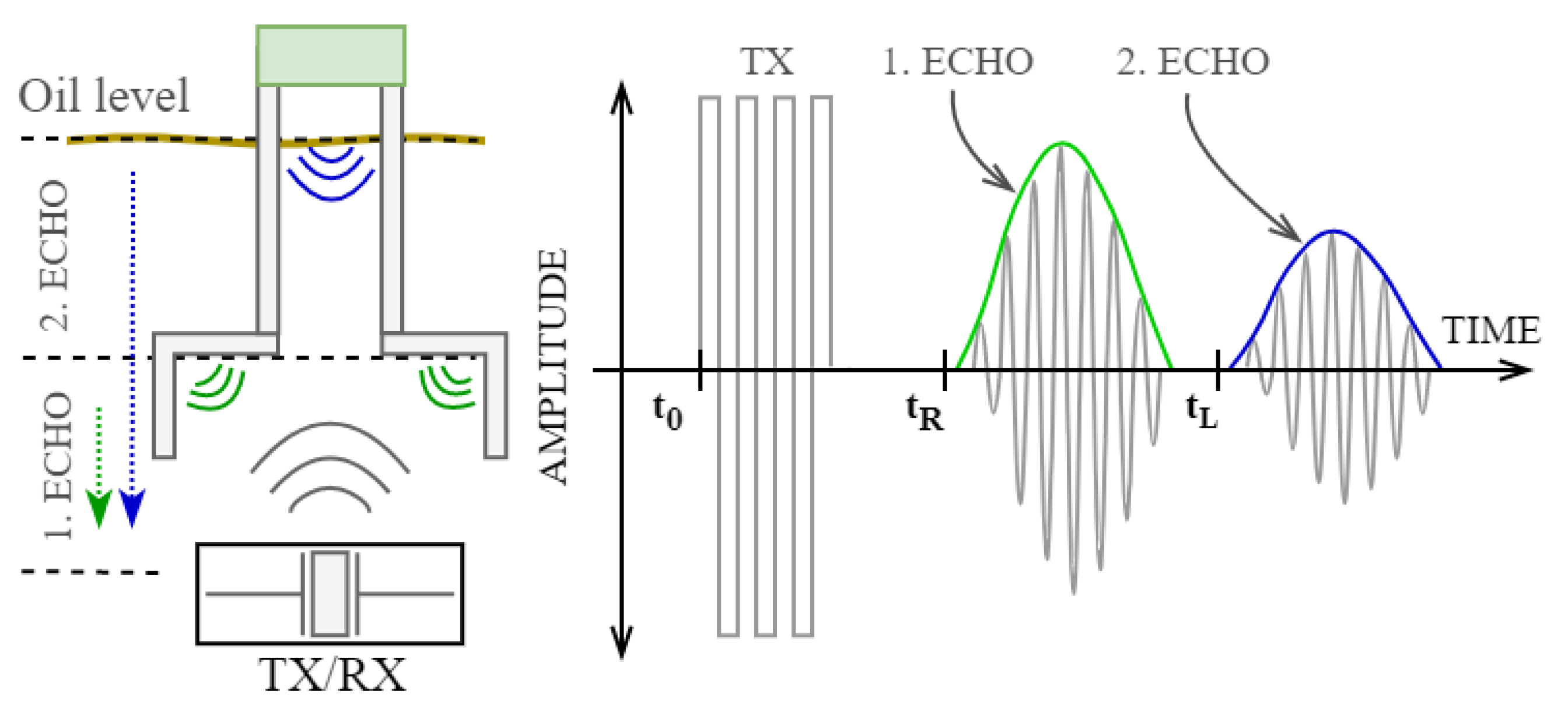
The ultrasonic measurement method is based on the principle of measuring the time of propagation of the ultrasonic signal on the surface and in the reverse direction. This includes knowledge of ultrasonic signal reflection, refraction and transition [37]. Based on this time, the height of the oil (liquid) level is calculated with the knowledge of the propagation velocity of the ultrasonic signal. Since the propagation velocity of the ultrasonic signal depends on the liquid type, temperature, and pressure, an auxiliary reference surface is used, which is located at a precisely defined distance from the source of the ultrasonic signal. The method of precise measurement consists in sending one ultrasonic pulse (burst) and measuring the time in which this pulse bounces off the reference surface and onto the surface. Based on the knowledge of the reflection time from the reference surface and its exact distance from the ultrasonic signal source, we can precisely calculate the propagation velocity of the ultrasonic signal. This calculated velocity already includes the effects of temperature, density, pressure, and more. The used principle of ultrasonic signal generation and measurement is shown in Figure 1.

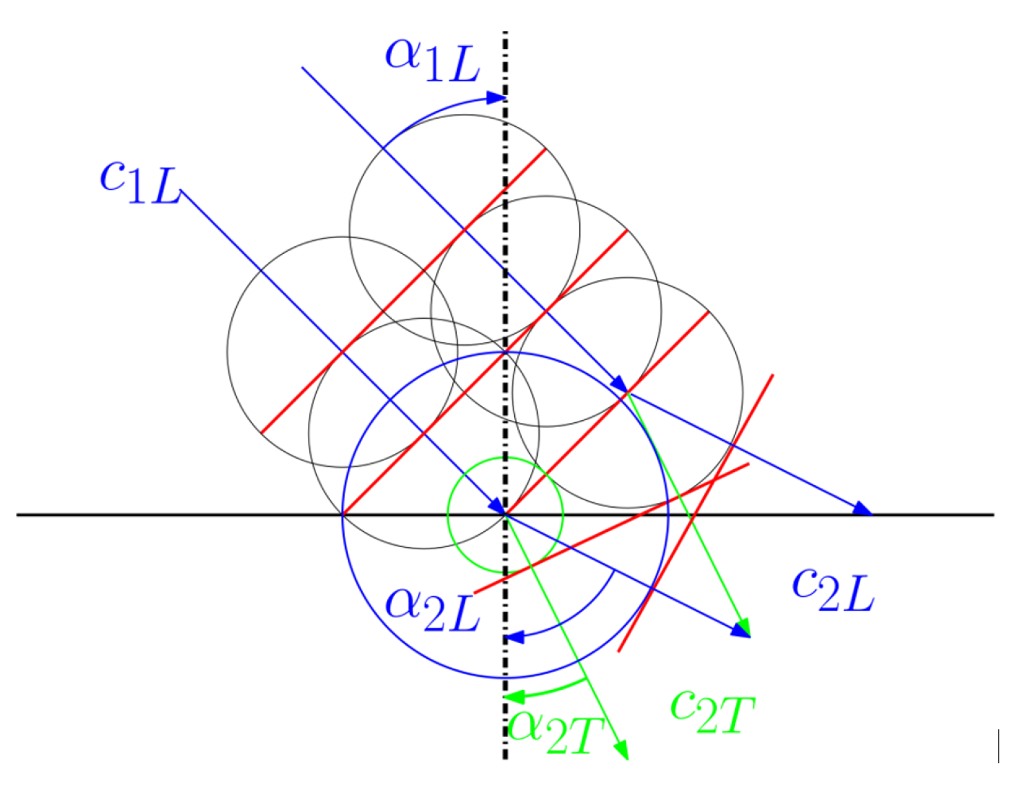
Now, it is possible to define the reflection and transmission coefficients for impacts at different angles—the essence is the vector nature of phase velocity. A Huygens principle is used, represented by Figure 2.

3.1. Sound Intensity Level and Sound Pressure

Due to the periodic nature of the acoustic pressure and speed of sound, we introduce the mean values $p_{ef}$, $v_{ef}$:

$$\begin{array}{c}{p}_{ef}=p_A\sqrt{\frac{1}{\pi }{\int }_{-\frac{\pi }{2}}^{\frac{\pi }{2}}{cos}^{2}tdt}=\\ \sqrt{\frac{1}{\pi }{\left[\frac{1}{2}t+\frac{1}{4}sin2t\right]}_{-\frac{\pi }{2}}^{\frac{\pi }{2}}}=p_A\sqrt{\frac{1}{2}}\\ v_{ef}=\frac{v_A}{\sqrt{2}}\end{array}$$

(1)

Assuming that the amplitude of the sound pressure is $p_A=c\rho \omega A$, then the intensity is given as:

$$I=\frac{1}{2}\frac{{p_A}^2}{c\rho }=\frac{{p_{ef}}^2}{c\rho }=c\rho {v_{ef}}^2=p_{ef}{v}_{ef}$$

(2)

We also introduce acoustic levels—they are not frequency-dependent, and therefore also apply in the field of ultrasound. The following applies to the sound intensity level and is given as:

$$\begin{array}{c}d{L}_1=g\frac{dI}{I}\\ L_I=gln\frac{I}{I0}=\frac{g}{loge}log\frac{I}{I_0}=10log\frac{I}{I_0},\end{array}$$

(3)

where k is an unspecified constant, so we can express $\frac{g}{loge}$ determined as 10, and solve everything by determining $I_0={10}^{-12}\mathrm{W}·{\mathrm{m}}^{-2}$, which is the intensity reference value at 1000 Hz.

We can determine the sound pressure level as:

$$L_p=20log\frac{p_{ef}}{p_0},$$

(4)

where $p_0=2\times {10}^{-5}\mathrm{Pa}$ is the reference value of the sound acoustic pressure. The sound power level is then defined as: $I=\frac{P}{S}$ and $I_0=\frac{P_0}{S}$, and is given as:

$$L_P=10log\frac{P_{ef}}{P_0},$$

(5)

where $P_0={10}^{-12}$ W is the reference value of acoustic power.

However, in a real environment, the measurement is never stable and the measurement values fluctuate depending on the characteristics of the environment and the physical behavior of the liquid in the vessel.

3.2. ANOVA Testing Method

One-way analysis of variance (ANOVA) [39] compares the means of two or more groups for one dependent variable. One-way ANOVA is necessary when a study involves more than two groups. For nominal groups, interval-dependent variables are required. The assumption of a normal distribution is not required [40].

The implemented ANOVA method on the measured data was chosen mainly due to the detection of significant differences between the variables representing the physical values of the received ultrasound signal with the set parameters of the environment.

4. Measurement

The measurement was performed with an ultrasonic level sensor with a measurement range of 20–100 mm and a temperature range of 0–150 °C. The measurement frequency of the sensor is 10 measurements per second. The transverse resonant frequency of the piezo element, which has a value of 10 MHz, is used to excite the ultrasonic signal.

Ultrasonic measurement was driven by a Renesas RL78/F13 CPU. The sensor that was tested was driven by a CPU with the experimental circuit described later on, and was mounted inside the test machine for level measurement accuracy testing. The test machine allows to fix the motor oil level and temperature, so it is a proper instrument for the requested experiment. In this study, the synthetic motor oil Shell Helix Ultra Professional AF 5W-30 was used. The measurement was performed by following motor oil levels and temperatures; see

Table 1. Overview of measurement conditions.

Variable	Unit	Measurement Points
Motor oil level	mm	20; 30; 40; 50; 60; 70; 80; 90; 100
Temperature	°C	−10; −5; 0; 35; 50; 70; 95; 130

.

The test machine was used only for modification of the temperature and motor oil level. The sensor was connected to the oscilloscope and via an oscilloscope to the PC that was equipped with the developed measurement software. Measurement data contained 3000 rows, so every row represented an individual measurement under defined conditions. All measurement data had a CSV format.

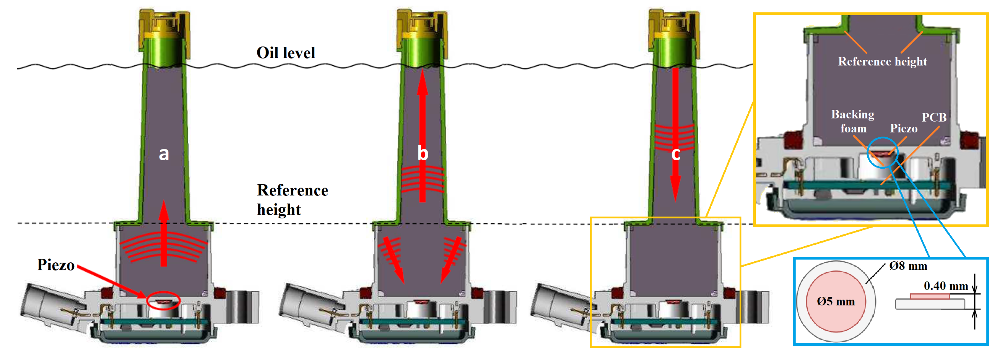
The maximum height of the reference surface is given by the requirements for the construction of the sensor and the minimum measurable height of the oil level. The sensor is placed at the bottom of the oil pan. It must be ensured that the reference surface is always immersed in oil. From the point of view of accuracy, it is advantageous to have the reference surface as far as possible from the source of the ultrasonic signal, i.e., the piezo element.

The ultrasonic sensor is designed to measure the motor oil level. It has a reference height to determine the exact value of the speed of sound. The measurement principle is based on ultrasonic reflection from the reference surface and level surface. The reason why the reference level measurement supplements the oil level measurement is mainly related to the actual physical and chemical parameters in the measured oil bath, where the response rate directly depends on these parameters. The speed of sound is changing rapidly based on the temperature of oil and its quality. For that reason, we are using the reference for precise sound measurement speed as we cannot predict the quality changes inside oil during its lifetime. The ultrasonic sensor construction and measurement principle are shown in Figure 3.

Ultrasonic pulse handling is driven by the CPU. The electronics for ultrasonic pulse handling contain an experimental circuit that is based on ultrasonic pulse energy saturation, which creates a logical value for the CPU. The principal solution for this circuit is shown in Figure 4 and it consists of:

• MCU —Generates a PWM signal, five pulses in total. The MCU output switches a transistor, the signal is in the range of 0–V${}_{cc}$ and V${}_{cc}$–0.
• Duplexer and Resonator—The circuit contains a filter with coils that provide resonance at 4 MHz.
• Amplifier—A simple transistor amplifier with variable gain.
• Detector—Detects the 4 MHz envelopes of the ECHO signal.
• Low-pass filter—Eliminates high frequencies from the signal for better readability of ECHO signals.
• Shaper—Detects ECHO signals using a transistor and threshold and connects V${}_{cc}$ to the output at that moment.
• MCU—The MCU detects the signal from the shaper, measures the length of the pulses and their number, and sends the data via UART to the LabView application.

For this study, measurement was performed using the oscilloscope Keysight MSO-X 2024A. The resolution setting of the oscilloscope was 10 $\mathsf{\mu }$S/particle and 100 mV/particle in the amplitude region. The oscilloscope was connected with a USB interface to a PC that was running a proprietary LabView application. Measured data were processed by the application and then stored in a CSV file. Each of the four channels of this oscilloscope was used:

• CH1: Amplified echo signal; these data were used for further offline analysis of the echo signal (statistical analysis);
• CH2: The pulse of HW electronic detection from the echo signal, which is used as the input of MCU echo detection; these data were used for further comparison of correct MCU detection (in comparison with UART data outputs);
• CH3: UART data (output of MCU measurements);
• CH4: NTC signal (detection of ambient temperature).

The schema of the whole measurement system is shown in Figure 4. In the middle part is the block diagram of the measurement chain. First, an initial pulse is generated in the CPU unit for the excitation of the piezo element. Echo signals detected by this piezo element are then amplified (at this point CH1 is connected), electronically detected, filtered, and shaped (at this point CH2 is connected). A shaped echo signal (ECHO pulse) is detected by the CPU unit and the processed data are transferred to a UART (Universal Asynchronous Receiver–Transmitter) communication interface (at this point CH3 is connected). CH4 is connected to the output of the NTC (Negative Temperature Coefficient) sensor. In Figure 4 can be seen the part of the electronic schema used for echo signal processing at the upper part and the demonstration of each signal involved in the whole measurement chain in the lower part.

5. Results

Measurements of the reflected ultrasonic signal were made at different oil heights and references. These measurements were compiled depending on the variable oil temperature and the selected oil type. The measured data shaped into an envelope of the received ultrasonic signal with specific amplitude were subjected to regression analysis and ANOVA analysis of inter-dependencies. The obtained dependency algorithms can be used to significantly refine and understand the envelope shaping of the received ultrasonic signal. Physically, it was assumed that the amplitude of the envelope of the received ultrasonic signal and its steepness are directly dependent on the height and temperature of the oil, but the selected analyses helped to pinpoint the inter-dependencies and thus enable more precise detection of the edge location of the received ultrasonic envelope. Below is a selected dataset on which the inter-dependencies and the resulting analyses by regression analysis and ANOVA analysis are presented.

If the motor oil level of 30 mm is mentioned, it is clear that there is almost no dependence between the amplitude of the reference and the temperature. On the other hand, the amplitudes of the level can be well described by the second-degree polynomials; see Figure 5a. In the case of the motor oil level of 60 mm, it can be said that temperature does not have a significant influence on the amplitude of reference. On the contrary, there is a clearly visible trend for the amplitude of the motor oil level that can be described by the second-degree polynomials; see Figure 5b. Measurement data analysis revealed very low amplitudes for both reference and level signals for temperatures that are close to zero. In the case of the reference signal, the amplitude is relatively stable. The amplitude of the level signal is constantly increasing up to a temperature of 100 °C. Amplitudes related to the motor oil level might be described quite well by the second-degree polynomials; see Figure 5c. In the given representation, the amplitude (mV) is denoted by the variable Y, while the temperature (°C) is represented by the variable X.

Experimental data related to $\Delta$t, amplitude starting from the level, slope of the level amplitude, and amplitude from the reference were selected according to the motor oil level in the level measurement device. Data were tested by one-way ANOVA (equal variances were not assumed). As can be seen, there is no statistically significant difference among the $\Delta$t groups. Amplitude start from the oil level revealed a statistically significant difference for the two pairs of 30–90 mm and 30–60 mm. Moreover, the slope exhibited a significantly different pair of variables (30–90 mm). Finally, the amplitude of reference did not show any statistically significant difference among all three groups.

In this way, selected data of variables representing the physical values of the received ultrasonic signal were analyzed to confirm the significant oil height-dependent differences in the variable temperature settings.

Regression Analysis Results

Regression analysis is a statistical method by which we estimate the value of some random variable called the dependent variable, also called the target variable, regressand, or explanatory variable, based on knowledge of other independent variables, regressors, covariates, or explanatory variables.

A typical mathematical method used to solve problems of this type is Pearson linear discriminant analysis, which is used in this case study.

Pearson correlation coefficient and relevant significance levels were calculated in Minitab 17 for the most important measurement variables. These experimental variables were motor oil level, amplitude related to the oil level, amplitude start value (determined manually), amplitude slope (shape of the level signal envelope), UART amplitude start value, pulse, and $\Delta$t. The correlation matrix revealed that there are very strong correlations among the following pairs: pulse–UART amplitude start, pulse–amplitude start, slope–amplitude level, pulse–level, and UART amplitude start–level. There are also statistically significant correlations between the pairs: amplitude level–level, slope–level, and UART amplitude start–amplitude level; see

Table 2. Correlation matrix of the most important experimental variables. All values in bold are significant ($p<0.05$).

Name	Unit	Level	AmplitudeLev	AmpStart	Slope	UARTAmpStart	Pulse
AmplitudeLev	mm	−0.736/0.000	-	-	-	-	-
AmpStart	$\mathsf{\mu }$s	0.967/0.000	−0.622/0.006	-	-	-	-
Slope	mV/$\mathsf{\mu }$s	−0.596/0.000	0.914/0.000	−0.444/0.065	-	-	-
UARTAmpStart	$\mathsf{\mu }$s	0.967/0.000	−0.620/0.006	1.000/0.000	−0.444/0.065	-	-
Pulse	$\mathsf{\mu }$s	0.967/0.000	−0.622/0.006	1.000/0.000	−0.447/0.063	0.999/0.000	-
dt	$\mathsf{\mu }$s	−0.183/0.468	0.036/0.887	−0.128/0.613	−0.266/0.286	−0.131/0.603	−0.121/0.632

.

For the descriptive statistics, we chose 18 data rows (each of them representing 30 fractional measurements). Low-temperature raw data were eliminated from the statistics due to outliers (90 mm; −0.1 °C) and/or incomplete data ensembles (58.5 mm and 80 mm; −5 °C and −10 °C). The descriptive statistics revealed that the average value of $\Delta$t is 1.5 ± 0.27 µs. In terms of oil level measurement accuracy, it was ±0.41 mm; see

Table 3. Descriptive statistics summary of the most important variables.

Variable	Unit	Total Count	Mean	StDev	Minimum	Median	Maximum	Range
dt	$\mathsf{\mu }$s	18	1.5072	0.2763	1.0100	1.5400	1.9500	0.9400
Offset	mV	18	0.00683	0.000786	0.00500	0.00700	0.00800	0.00300
Slope	mV/$\mathsf{\mu }$s	18	0.03366	0.01444	0.00455	0.03647	0.06776	0.06322
AmplitudeLev	mV	18	0.05789	0.02838	0.00700	0.05550	0.10300	0.09600
AmplitudeRef	mV	18	0.01283	0.001383	0.01100	0.01100	0.01600	0.00500

.

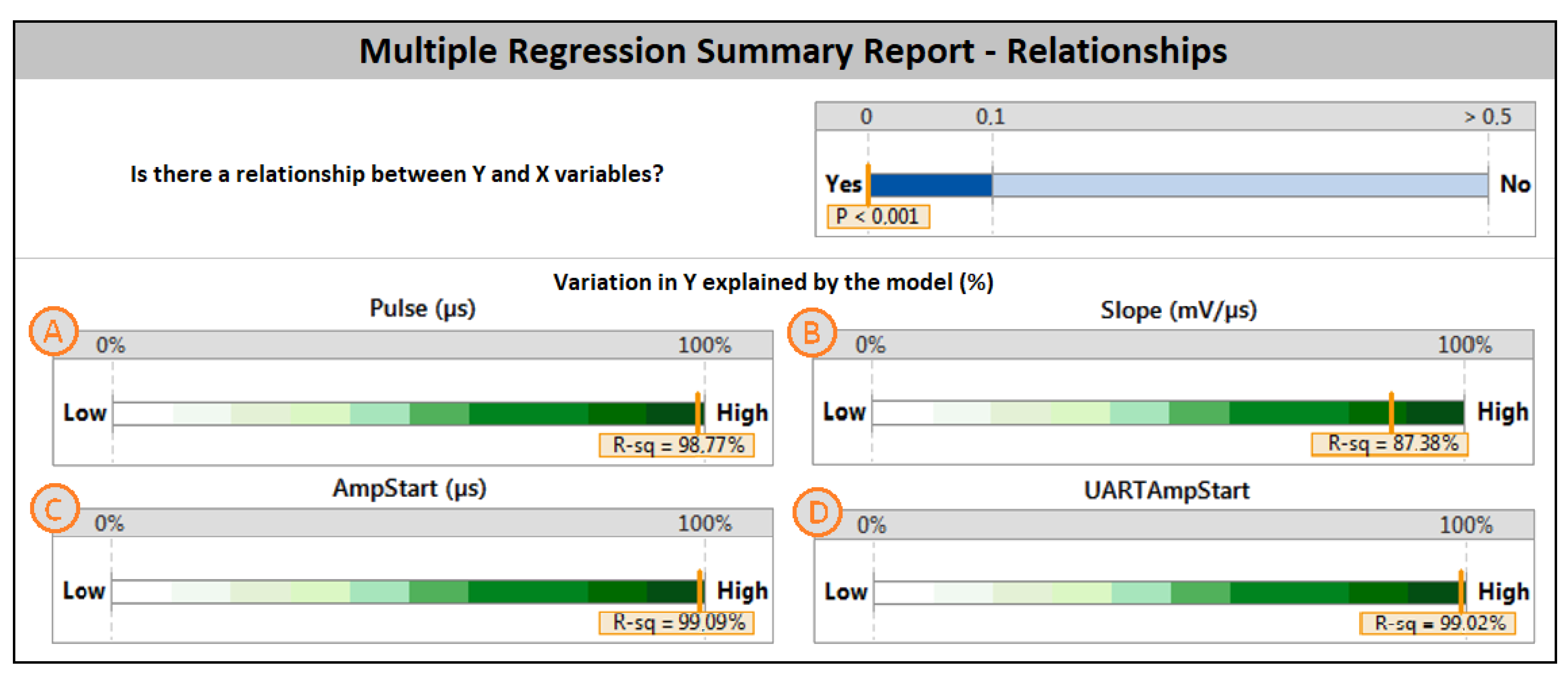
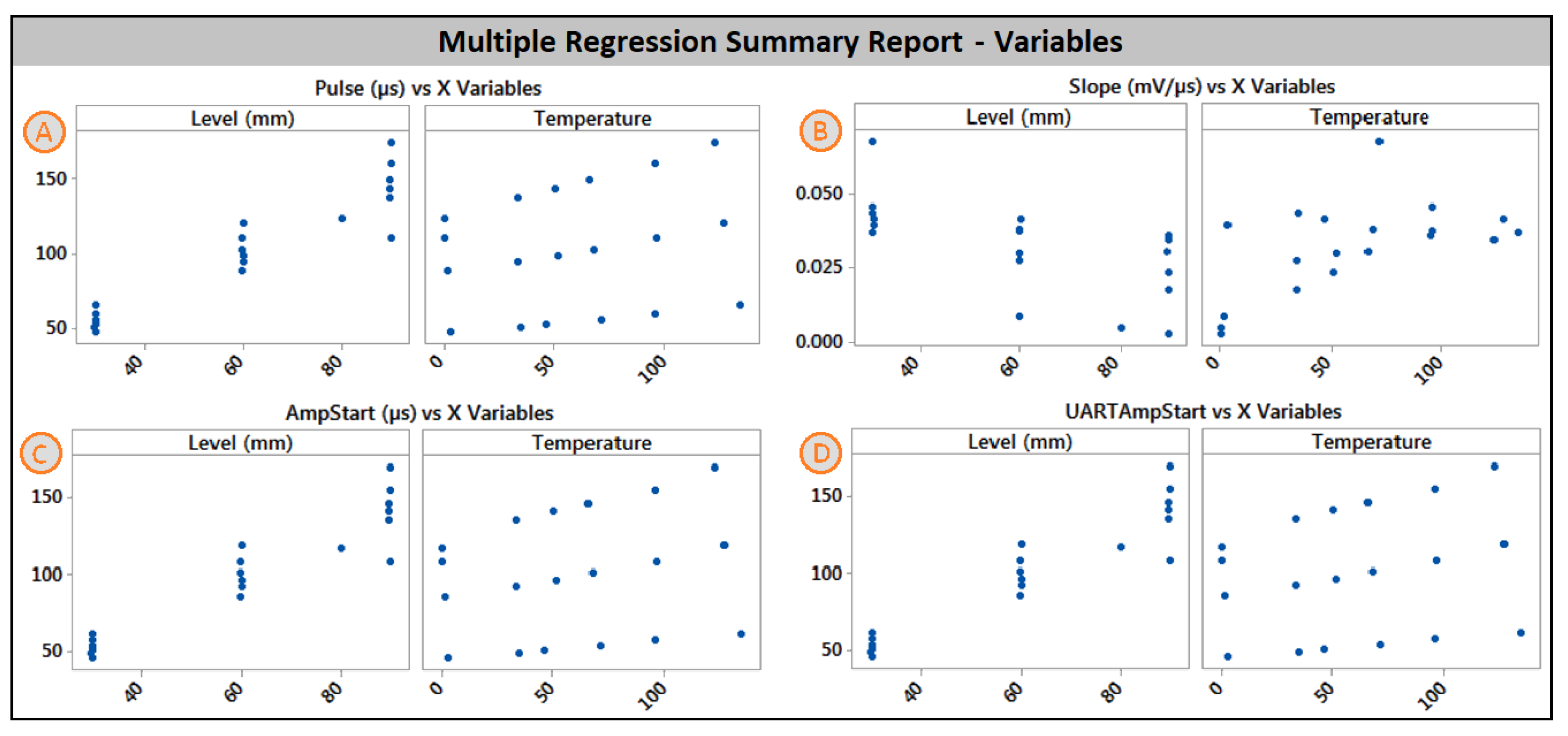
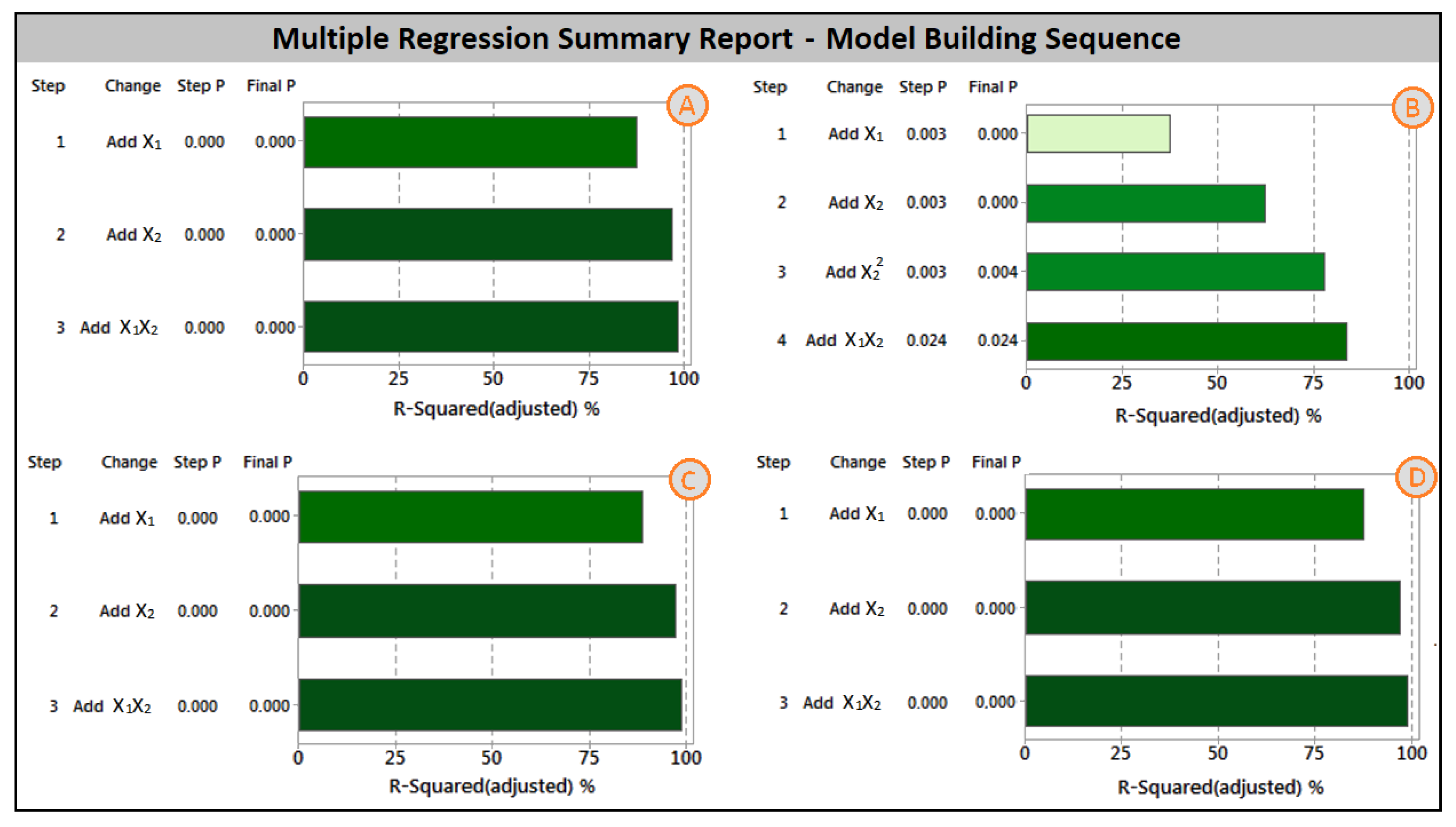
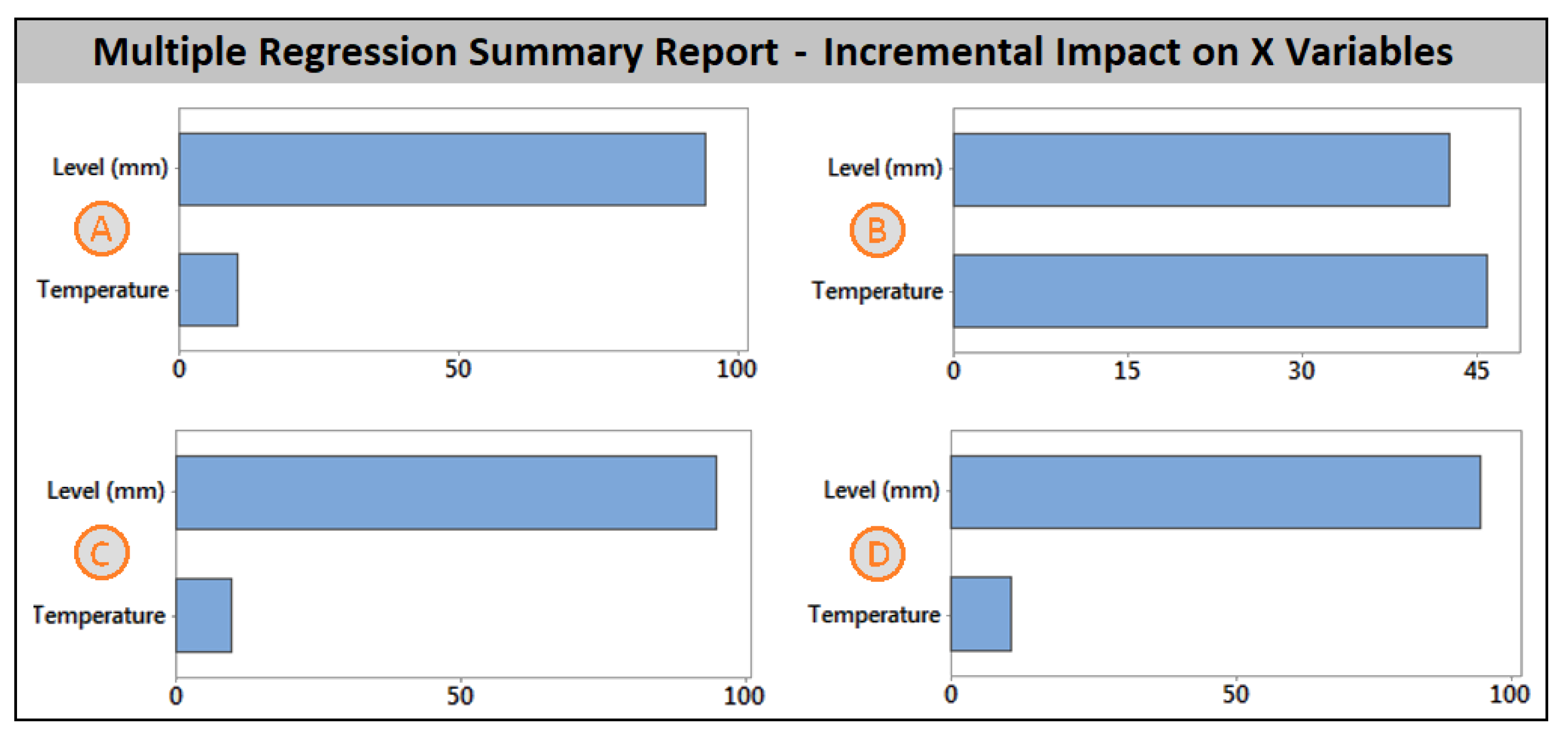
Another step was multiple linear regression analysis. This type of analysis allowed us to determine the functional dependency of the crucial variables on motor oil level and temperature. The multiple linear regression model consists of the following information: statistical significance, the percentage of variation that might be explained by the model, and the final model equation. In the case of the multiple regression for amplitude level, it can be seen that the explanation strength of the model is very high; see Figure 6—top/right.

On the contrary, $\Delta$t cannot be explained by the regression model at all. Meanwhile, the explanation strength of the regression model for $\Delta$t was equal to zero, and the Pulse start variable might be completely described by the following regression model; see Figure 6, Figure 7 and Figure 8 and Figure 9A. Good explanation strength of the regression model was achieved for the Amplitude Slope; see Figure 6, Figure 7 and Figure 8 and Figure 9B.

Both the Amplitude Start and UART Amplitude Start variables showed very high explanation strength in terms of multiple regression models; see Figure 6, Figure 7 and Figure 8 and Figure 9C,D. On the contrary, the offset value, typically 0.007 mV for most of the experimental conditions, revealed that there was no statistically significant relation between the offset value and the input variables (motor oil level and temperature). Detailed information about the measured values can be found in

Table 4. Description of measured parameters.

Signal	Unit	Meaning
$Level$	mm	This is the actual level of the measured oil.
$AmplitudeLev$	mV	It is an echo echo amplitude of the ultrasonic signal reflected from the oil surface. It is the maximum measured value on the receiving piezo element.
$AmpStart$ (C)	$\mathsf{\mu }$s	This is the time delay calculated from the moment the ultrasonic signal is sent from the exciter to its return. It is the time of flight of the ultrasonic signal that is measured by the oscilloscope.
$Slope$ (B)	mV/$\mathsf{\mu }$s	This is the steepness of the front of the reflected ultrasonic signal.
$UARTAmpStart$ (D)	$\mathsf{\mu }$s	This is the time delay calculated from the moment the ultrasonic signal is sent from the exciter to its return. It is the time of flight of the ultrasonic signal, which is measured by the microprocessor from the discretized ultrasonic signal.
$Pulse$ (A)	$\mathsf{\mu }$s	This is the time length of the discretized received echo of the ultrasonic signal.

.

Experimental data related to the $\Delta$t, amplitude starts from the level, slope of the level amplitude, and amplitude from the reference were selected according to the motor oil level in the level measurement device. Data were tested by one-way ANOVA (equal variances were not assumed). There are no statistically significant differences among the $\Delta$t groups. Amplitude start from the oil level revealed statistically significant differences for the two pairs 30–90 mm and 30–60 mm. Moreover, the slope exhibited a significantly different pair of variables (30–90 mm). Finally, amplitude from the reference did not show any statistically significant difference among all three groups.

Multiple regression model results can be seen in Equation (6).

$$\begin{array}{c}\hfill \begin{array}{cc}\hfill \left(A\right)& :Pulse\left(\mathsf{\mu }\mathrm{s}\right)=10.21+1.2511·X_1-0.0247·X_2+0.00483·X_1{X}_2\hfill \\ \hfill \left(B\right)& :Slope(\mathrm{mV}/\mathsf{\mu }\mathrm{s})=0.05147-0.000599·X_1+0.000333·X_2+0.000003·{X_2}^2+0.000004·X_1{X}_2\hfill \\ \hfill \left(C\right)& :AmpStart\left(\mathsf{\mu }\mathrm{s}\right)=7.96+1.2010·X_1-0.0211·X_2+0.004659·X_1{X}_2\hfill \\ \hfill \left(D\right)& :UARTAmpStart(-)=9.06+1.2283·X_1-0.0263·X_2+0.004745·X_1{X}_2\hfill \\ & X_1:\mathrm{Oil}\mathrm{Level}{X}_2:\mathrm{Oil}\mathrm{Temperature}\hfill \end{array}\end{array}$$

(6)

6. Discussion

The present study aimed to investigate the relationship between external conditions, such as motor oil level and temperature, and the amplitude of the reference and oil surface signals in ultrasonic measurements. The results show that the amplitude of the reference signal was not affected by external conditions, while the amplitude of the oil surface signal was weak when the oil temperature was around −10 °C. Temperatures within the range of −5 °C to 140 °C should not pose any problem in terms of detection and evaluation. When very low temperatures are mentioned (−10 °C), the signal from the piezo element was strongly dimmed due to the motor oil’s physical properties, but the signal from the reference was still detected.

Furthermore, the amplitude of the ultrasonic echo signal was found to be related not only to the liquid level height and temperature but also to the characteristics of the probe. Specifically, in low temperatures, the probe’s characteristics were found to change greatly, which directly affected the strength of the received ultrasonic signal. Regression analysis demonstrated that the amplitude measured by the ultrasonic signal electronics could accurately describe the physical state of the oil level and its temperature, with an accuracy of 99.02% compared to the amplitude measured directly on the piezo element of the ultrasonic signal receiver, where the agreement was only 97.94%.

The discrepancy in accuracy was attributed to the ultrasonic signal being preprocessed by an active envelope detector with variable gain before actual measurement by the sensor electronics, which was further filtered by a low pass filter and a shaper. Overall, the present study suggests that the tested type and sensor design can perform measurements with higher than 99% accuracy, as the envelope of the ultrasonic signal accurately reflects the relationship with the level and temperature of the oil.

However, it must be mentioned that only raw data were used in the study, and automatic filter usage may further improve the already good raw data results. Moreover, at room temperature or higher, the amplitude of the oil surface signal was found to increase up to 100 °C, after which it slightly decreased. The amplitude of the oil surface behavior was also well-predicted by second-degree polynomials. Regression analysis, correlation, and one-way ANOVA testing contributed to a better understanding of these relationships and can be utilized in future research.

Temperature changes in the oil impact its physical properties, including density and viscosity. These changes affect the propagation characteristics of the signal, potentially leading to variations in the measured amplitude.

One aspect affected by temperature is the speed of sound in the oil medium. Generally, as temperature increases, the speed of sound in a material tends to increase as well. This change in speed influences the amplitude of the signal received during ToF measurements. However, it is worth noting that the amplitude is not directly proportional to temperature but rather influenced by the changes in the medium’s properties caused by temperature.

Moreover, temperature fluctuations can also introduce additional noise or interference to the signal, which can impact the accuracy of ToF measurements. Proper compensation or calibration techniques may be required to account for temperature-related effects and ensure accurate oil level measurements.

Time of flight is a measured parameter that represents the time interval from the emission of the initial burst until the reception of the leading edge of the corresponding echo signal.

Precise measurement of oil level is critical to maintain the requisite tolerance bands in a real-world setting, particularly under degraded measurement conditions. When measuring oil level in the engine compartment, an accurate level measurement is especially advantageous when the vehicle is parked on an inclined surface with a level inclination, such as a hill, as a more sensitive measurement system can significantly improve the accuracy of oil level determination. In cases where the oil level measurement is non-functional during engine start-up, or during prolonged uphill or downhill driving, incorrect measurement can cause the engine to switch to emergency mode and limit its performance to avoid damage.

The findings of oil level measurement can also be applied in verification and calibration measurements, as well as other specialized applications, across different domains.

7. Conclusions

This work brings a better understanding of the behavior of the ultrasonic signal inside the sensor and the factors that affect its behavior. At the same time, this work describes the relationships of individual physical quantities (amplitude, runtime, etc.). Based on this, the system of sensor validation and setting of some calibration parameters was modified, which ultimately led to an increase in the reliability of measurement by the sensor, which is used in cars. The measurement accuracy of the oil level was improved by adaptation of the setting of the measurement’s parameters, specifically the amplification of receiving echo based on oil temperature. which increases the accuracy of the measurement across the whole temperature range.

One significant improvement achieved through this research is the enhanced accuracy of oil level measurements. By adapting the measurement parameters, particularly by amplifying the received echo based on oil temperature, the measurement accuracy is improved across the entire temperature range. Statistical methods such as ANOVA and regression analysis were employed to adjust the amplitude of the envelope, leading to increased sensitivity in detecting the envelope height threshold. By utilizing this approach, the researchers were able to precisely describe the temperature dependence and effectively minimize it in the measurements.

In addition to the improvements made to the measurement accuracy, the study also investigated the possibility of reducing the effects of temperature on the signal envelope. The researchers found that the signal envelope is strongly affected by temperature, which can lead to errors in the measurement. However, by using statistical methods to modify the appearance of the detected envelope, it was possible to reduce this dependence to a negligible minimum.

The study also found that the characteristics of the probe used can have a significant impact on the accuracy of the measurement. The researchers suggest that further improvements can be achieved by developing more sophisticated probes, or by optimizing the existing probes to reduce the effects of environmental factors such as temperature and humidity.

Overall, the study provides valuable insights into the behavior of ultrasonic signals and their application in automotive sensors. By improving the reliability and accuracy of these sensors, it is possible to enhance the safety and efficiency of automobiles, and to provide better feedback to drivers about the status of their vehicles.

The significance and value of this study also is that measurement precision can be compensated for without knowledge of other parameters. The performed regression analysis shows a strong dependence on the temperature and level of the oil, and the envelope of the reflected signal depends on the level and temperature of the oil.

In conclusion, this research holds important implications for the automotive industry, serving as a foundation for further advancements in the field of oil level measurement. By continually refining the technology employed in automotive sensors, vehicles can become safer, more efficient, and more reliable.

Through the optimization process, the accuracy of the sensor has been significantly improved, surpassing 99%. This optimization has effectively addressed the sensor’s issues related to inclination. The improvements made have successfully eliminated any problems or inaccuracies associated with the sensor’s performance under inclined conditions. As a result, the sensor now provides highly accurate measurements even in situations where inclination was previously a challenge.

8. Patents

The presented results are covered by a registration with the Industrial Patent Office of the Czech Republic under application number 2019-35923 entitled: “A device for measuring the level and concentration of liquids”.