Investigating the Non-Gaussian Property and Its Influence on Extreme Wind Pressures on the Long-Span Cylindrical Roof

Abstract

The non-Gaussian property and its influence on peak factors and extreme wind pressures on the long-span cylindrical roof are studied in this paper. Firstly, the moment-based Hermite polynomial model (HPM), which is used to determine peak factors of non-Gaussian processes, is briefly introduced. Then, wind tunnel tests for the scaled rigid roof model are carried out to measure wind pressures on the roof surface. The statistical and spatial distribution of non-Gaussian properties of wind pressure on the roof is demonstrated. Regions around curved edges along the span of the roof exhibiting strong non-Gaussian properties are found. Peak factors determined by the HPM are examined by wind tunnel results and then calculated for the entire roof. According to their distribution, the regions with considerable peak factors are found. Results indicate that the peak factor of constant 2.5 or peak factor following the Gaussian process assumption is far smaller than that determined by the HPM, leading to extreme wind pressures being underestimated by 40–50%. Hence, it is necessary to include the non-Gaussian properties of wind pressure when calculating their extreme values for such long-span cylindrical roofs.

1. Introduction

Wind loads on long-span roofs are always critical concerns at the structural design stage. Therefore, an accurate evaluation of the extreme wind pressure on the roof is essential. At present, the peak factor following classical Gaussian assumption is often accepted to determine extreme values of wind pressures. In most codes [1,2,3,4,5], peak factors are suggested as 2–4. For example, a peak factor of 2.5 is used in the Chinese standard GB50009-2019 [5]. However, this is not the case for actual peak factors for wind pressures on long-span roofs.

Generally, most regions of the long-span roof are immersed in flow separation. Pressures for these regions tend to exhibit non-Gaussian properties whose distribution tails are wider than Gaussian distribution [6,7]. Peak factors for non-Gaussian processes are often larger than those for Gaussian processes [8]. Still, using peak factors following the Gaussian assumption will underestimate the extreme values of wind pressures which leads to risky design or even undesirable roof damage [9,10,11].

There are two major ways to determine the peak factors and extreme values for non-Gaussian processes. One is the observed peak method [12,13,14,15]. This method relies on a large number of repeated samples to ensure accurate and precise data fitting, which is time-consuming and uneconomical in wind tunnel tests. The other is the translation process method, which uses a monotonic translation process to realize the translation of a non-Gaussian process to a standard Gaussian process. It establishes a point-to-point relationship between the non-Gaussian and Gaussian processes. The accuracy of the translation process method based on the Hermite polynomial model (HPM) and using short-term time histories to calculate peak factors has been verified by several studies [16,17,18].

There are relevant studies about non-Gaussian peak factors and extreme wind pressures for tall buildings [19,20,21,22,23] and small-size low buildings [24,25,26,27], while few studies are available for long-span structures with spans of hundreds of meters [28]. The cylindrical long-span roof is a very common building envelope for industrial structures. As shown in Figure 1, an L-shaped structure is the combination of a big cylindrical roof (BCR) and a small cylindrical roof (SCR). Nevertheless, the wind flow over a combined cylindrical roof considerably differs from that over a single cylindrical roof [29,30]. However, comprehensive statistical and spatial information about the non-Gaussian property and peak factors for the entire wind pressure field on the long-span roof is still not available but is critical for identifying the most sensitive regions on the roof.

This study focuses on the non-Gaussian property and its influences on peak factors and extreme values of wind pressure on the combined L-shaped long-span cylindrical roof and is organized as follows: the translation process method based on the HPM is first introduced. Then, wind tunnel tests are conducted to measure wind pressure histories for the roof. Subsequently, the non-Gaussian property of wind pressures is analyzed by the statistical and spatial distribution for mean value, skewness, and kurtosis of wind pressures. Finally, the peak factors and extreme values of wind pressures are investigated by different methods to illustrate the influence of the non-Gaussian property.

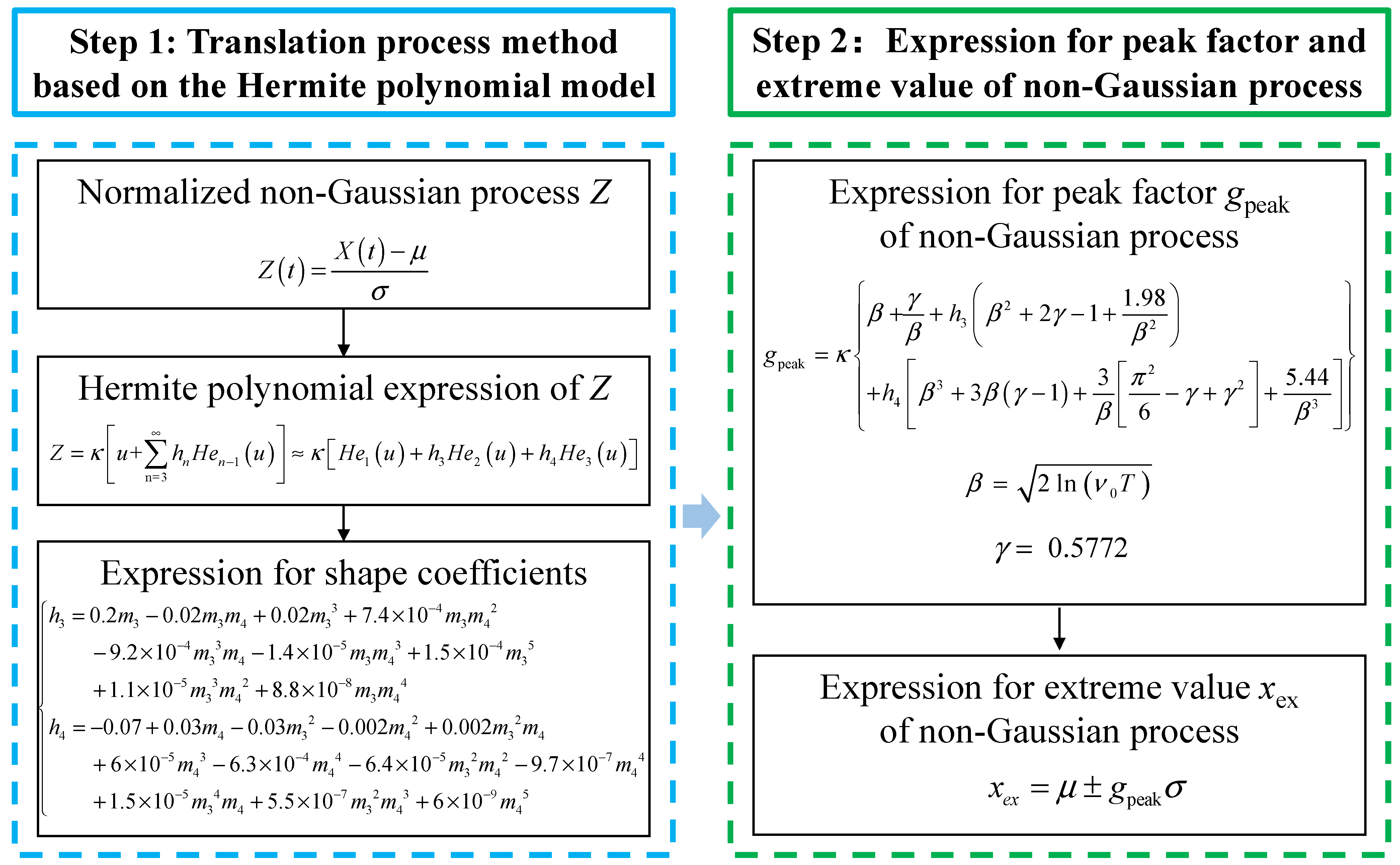
2. Methodology for Calculation of Peak Factors and Extreme Values

In this section, the translation process method based on the HPM is briefly introduced and employed to determine peak factors and extreme values of softening non-Gaussian wind pressures.

Supposing a non-Gaussian process X(t), the normalization of X(t) is:

$$Z\left(t\right)=\frac{X\left(t\right)-\mu }{\sigma },$$

(1)

where μ is the mean value and σ is the standard deviation of X(t). Z(t) can be expressed as a translation of a normalized Gaussian process U(t) using:

$$U(t)=g^{-1}\left(Z\left(t\right)\right),$$

(2)

where g(•) is a translation function. Then, the cumulative distribution function (CDF) of Z(t) is determined by:

$$F_{{\mathrm{z}}_{\mathrm{ex}}}\left(z\right)=\exp \left\{-{\nu }_{0}T\exp \left[-\frac{g^{-1}\left(z\right)}{2}\right]\right\},$$

(3)

and the probability density function p is determined by:

$$p_{{\mathrm{z}}_{\mathrm{ex}}}\left(z\right)=\exp \left(-\psi \right)\frac{d\psi }{dz},\begin{array}{c}\end{array}\psi ={\nu }_{0}T\exp \left[-\frac{g^{-1}\left(z\right)}{2}\right].$$

(4)

Here, the subscript z_ex represents the extreme value of Z(t) during the time T, and ν₀ is the mean zero up-crossing rate, which can be determined by spectral moments as:

$${\nu }_0=\sqrt{{\displaystyle {\int }_0^{\infty }{f}^2{S}_{\mathrm{z}}\left(f\right)df}/{\displaystyle {\int }_0^{\infty }{S}_{\mathrm{z}}\left(f\right)df}},$$

(5)

where S_z(f) is the auto-power spectral density of Z and f is the frequency in hertz. Accordingly, the expression of g(•) is decided, and thus the CDF for Z(t) is determined.

For hardening processes, whose kurtosises are less than 3, the peak factors are often smaller than those of the Gaussian processes. Peak factors calculated using Davenport’s equation result in conservative extreme results thereof. However, kurtosis for most wind pressures on long-span roofs is larger than 3, indicating a softening process whose peak factor is larger than that of a Gaussian process. Therefore, the softening processes are of great concern in this study.

The softening process Z can be expressed by the Hermite polynomial function of U as:

$$Z=g\left(u\right)=He\left(u\right)=\kappa \left[u+{\displaystyle \sum _{\mathrm{n}=3}^{\infty }{h}_{n}H{e}_{n-1}\left(u\right)}\right]\approx \kappa \left[H{e}_1\left(u\right)+h_{3}H{e}_2\left(u\right)+h_{4}H{e}_3\left(u\right)\right],$$

(6)

where $\kappa =\sqrt{1+2h_3^2+6h_4^2}$. h_n is the shape coefficient, and He_n(u) is the n-th order of the Hermite polynomial function which is expressed as:

$$H{e}_n\left(u\right)={\left(-1\right)}^n\cdot \exp \left(-\frac{u^2}{2}\right)\frac{d^n}{d{u}^n}\left[\exp \left(-\frac{u^2}{2}\right)\right].$$

(7)

Here, n = 1, 2, and 3 are substituted to Equation (7), respectively. He₁(u), He₂(u), and He₃(u) can be derived as:

$$H{e}_1\left(u\right)=u,H{e}_2\left(u\right)=u^2-1,\mathrm{and}H{e}_3\left(u\right)=u^3-3u.$$

(8)

Then, Equation (8) is substituted to Equation (6). Z can be derived as:

$$Z=g\left(u\right)=\kappa \left[u+h_3(u^2-1)+h_4\left(u^3-u\right)\right].$$

(9)

By these means, the expression of Equation (2) is termed the moment-based Hermite expression. Thus, g⁻¹(•) is derived as:

$$U=g^{-1}\left(Z\right)={\left[\sqrt{{\zeta }^2\left(z\right)+c}+\zeta \left(z\right)\right]}^{1/3}-{\left[\sqrt{{\zeta }^2\left(z\right)+c}-\zeta \left(z\right)\right]}^{1/3}-a,$$

(10)

where $\zeta \left(z\right)=1.5b\left(a+\frac{z}{\kappa }\right)-a^3$, $a=\frac{h_3}{3h_4}$, $b=\frac{1}{3h_4}$ and $c={\left(b-1-a^2\right)}^3$. To make g(•) always monotonically increasing, its slope ought to be positive, leading to:

$$h_3^2-3h_4(1-3h_4)\le 0.$$

(11)

The nth-order Hermite polynomial He_n(z) can be expanded at κu using Taylor’s theorem as follows:

$$H{e}_n\left(z\right)=H{e}_n\left(\kappa u\right)+{\displaystyle \sum _{j=1}^m\frac{H{e}_n{}^{\left(j\right)}\left(\kappa u\right)}{j!}}{\left[\kappa h_{3}H{e}_2\left(u\right)+\kappa h_{4}H{e}_3\left(u\right)\right]}^j$$

(12)

where $H{e}_{\mathrm{n}}{}^{\left(j\right)}=nH{e}_{\mathrm{n}-1}$ is the jth-order derivative of He_n. Take the first four terms of the expansion in Equation (12) into consideration. Shape coefficients h₃ and h₄ are determined by skewness m₃ and kurtosis m₄ of the following process:

$$\left\{\begin{array}{l}{m}_3={\kappa }^3\left(6h_3+36h_3{h}_4+8h_3^3+108h_3{h}_4^2\right)\\ m_4={\kappa }^4\left(3+24h_4+60h_3^2+252h_4^2+576h_3^2{h}_4+1296h_4^3+60h_3^4+2232h_3^2{h}_4^2+3348h_4^4\right)\end{array}\right..$$

(13)

Theoretically, as soon as the skewness m₃ and kurtosis m₄ are determined, h₃ and h₄ can be calculated by solving Equation (13). Nevertheless, Equation (13) is a system of non-linear simultaneous and implicit equations for h₃ and h₄. For calculation efficiency and application, an explicit expression for h₃ and h₄ is more favorable. To this end, an approximate explicit expression for h₃ and h₄ is proposed [31]:

$$\left\{\begin{array}{l}{h}_3=\frac{m_3}{6}\left[\frac{1-0.015\left|m_3\right|+0.3m_3{}^2}{1+0.2\left(m_4-3\right)}\right]\\ h_4=h_{40}\left[1-\frac{1.43m_3{}^2}{m_4-3}\right],\begin{array}{c}\end{array}{h}_{40}=\frac{\left[1+1.25{\left(m_4-3\right)}^{1/3}\right]-1}{10}\end{array}\right.(3<m_4<15)$$

(14)

However, the accuracy of Equation (14) cannot be guaranteed when process Z has strong non-Gaussian properties. Therefore, another approximate expression for h₃ and h₄ is proposed:

$$\left\{\begin{array}{ll}{h}_3=& 0.2m_3-0.02m_3{m}_4+0.02m_3{}^3+7.4\times {10}^{-4}{m}_3{m}_4{}^2\\ & -9.2\times {10}^{-4}{m}_3{}^3{m}_4-1.4\times {10}^{-5}{m}_3{m}_4{}^3+1.5\times {10}^{-4}{m}_3{}^5\\ & +1.1\times {10}^{-5}{m}_3{}^3{m}_4{}^2+8.8\times {10}^{-8}{m}_3{m}_4{}^4\\ h_4=& -0.07+0.03m_4-0.03m_3{}^2-0.002m_4{}^2+0.002m_3{}^2{m}_4\\ & +6\times {10}^{-5}{m}_4{}^3-6.3\times {10}^{-4}{m}_4{}^4-6.4\times {10}^{-5}{m}_3{}^2{m}_4{}^2-9.7\times {10}^{-7}{m}_4{}^4\\ & +1.5\times {10}^{-5}{m}_3{}^4{m}_4+5.5\times {10}^{-7}{m}_3{}^2{m}_4{}^3+6\times {10}^{-9}{m}_4{}^5\end{array}\right.$$

(15)

The above expression has been verified as accurate by wind tunnel test results in this study. It is applicable for strong non-Gaussian processes. Therefore, Equation (15) is adopted for calculations of shape parameters h₃ and h₄.

After h₃ and h₄ are determined, the CDF and PDF for z_ex in Equations (3) and (4) can be determined. Thus, a p-fractile of the extreme value for Z can be calculated from U according to the translation process method following:

$$z_{\mathrm{ex}}=g(u_{\mathrm{ex}}),u_{\mathrm{ex}}=\sqrt{2\ln \left[{\nu }_{0}T/\ln \left(1/p\right)\right]}$$

(16)

The expectation of z_ex is the peak factor g_peak, which has a form of

$$g_{\mathrm{peak}}=z_{\mathrm{ex},\mathrm{mean}}={\displaystyle {\int }_0^{\infty }{z}_{\mathrm{ex}}{p}_{\mathrm{ex}}(z)dz}.$$

(17)

g_peak corresponding to a 57% percentile can be derived as:

$$g_{\mathrm{peak}}=\kappa \left\{\beta +\frac{\gamma }{\beta }+h_3\left({\beta }^2+2\gamma -1+\frac{1.98}{{\beta }^2}\right)+h_4\left[{\beta }^3+3\beta \left(\gamma -1\right)+\frac{3}{\beta }\left[\frac{{\pi }^2}{6}-\gamma +{\gamma }^2\right]+\frac{5.44}{{\beta }^3}\right]\right\}$$

(18)

where $\beta =\sqrt{2\ln \left({\nu }_{0}T\right)}$, and $\gamma =0.5772$ is Euler’s constant. With this, peak factors for non-Gaussian processes can be calculated by Equation (18).

In addition, it should be noted that when m₃ = 0 and m₄ = 3, h₃ and h₄ are zero. Thus, Equation (18) degrades as:

$$g_{\mathrm{peak},G}=\beta +\frac{\gamma }{\beta }=\sqrt{2\ln \left({\nu }_{0}T\right)}+\frac{\gamma }{\sqrt{2\ln \left({\nu }_{0}T\right)}},$$

(19)

which is accordingly the peak factor expression for the Gaussian process.

The extreme value of a general non-Gaussian process X can be calculated as follows:

$$x_{ex}=\mu \pm g_{\mathrm{peak}}\sigma .$$

(20)

It is worth mentioning that Equation (20) is only applicable for obtaining a positive peak factor; when the mean value of X(t) is negative, the time history of X(t) should be multiplied by −1 to calculate the corresponding peak factor. The flowchart of the HPM is illustrated in Figure 2.

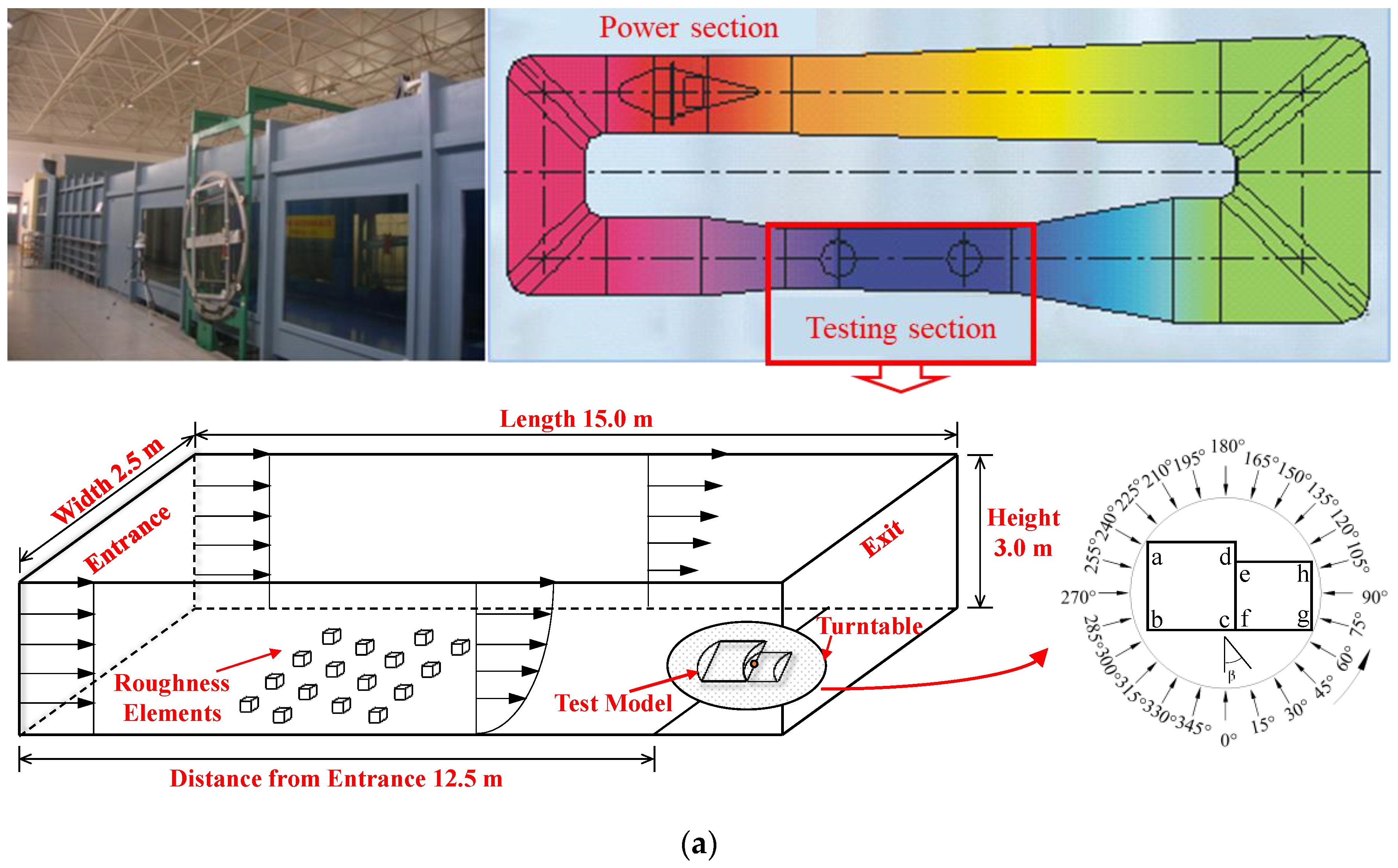
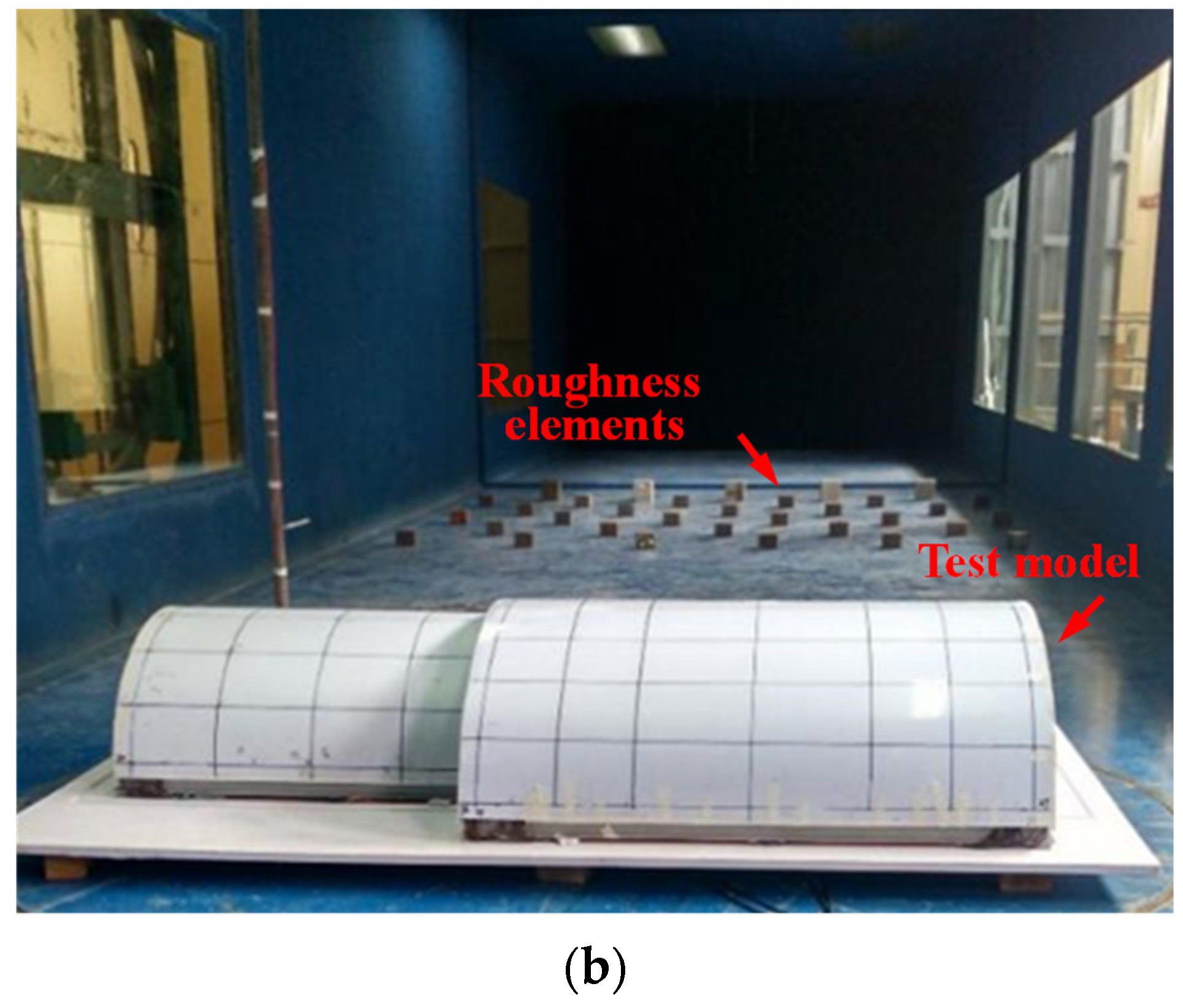
3. Wind Tunnel Tests

In this section, wind tunnel tests are conducted to obtain wind pressure histories for the scaled L-shaped model envelope.

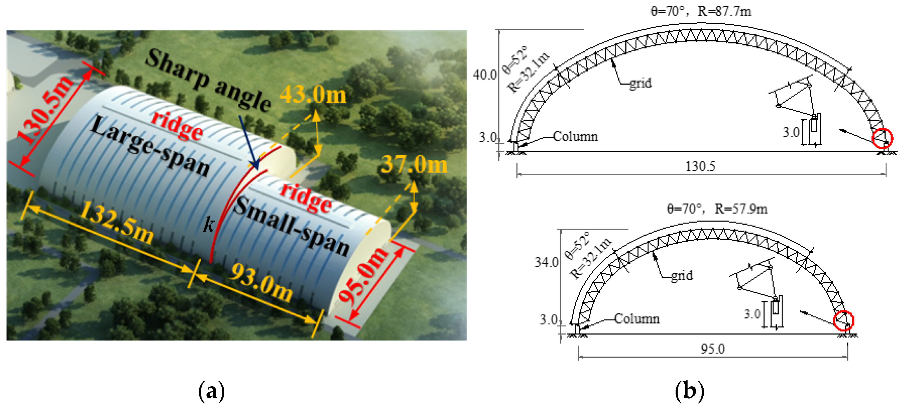
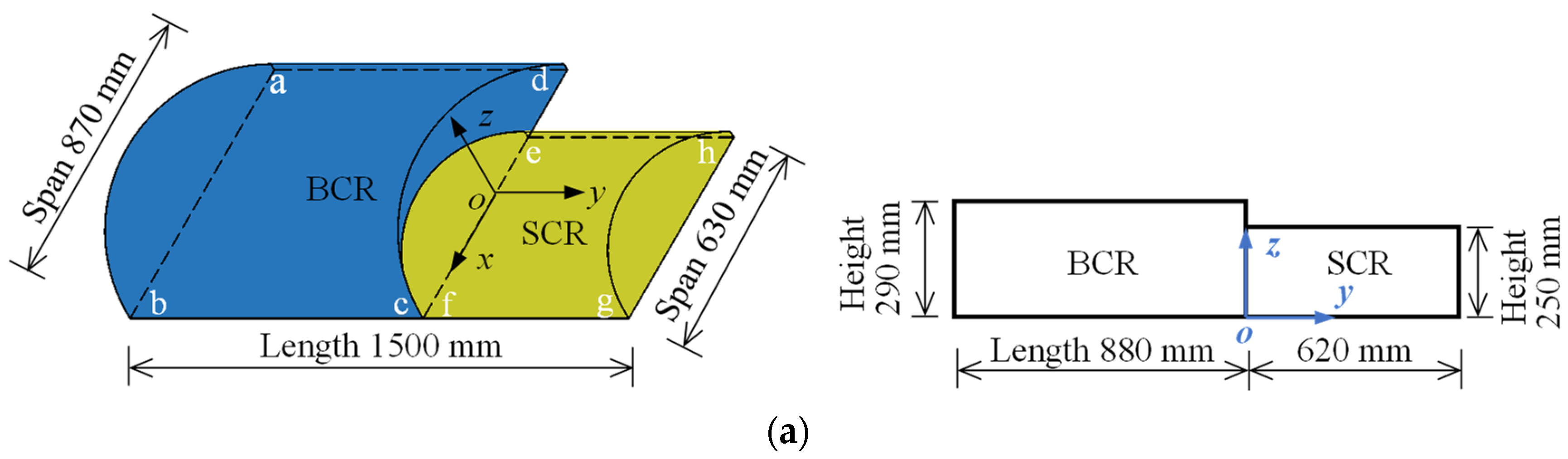
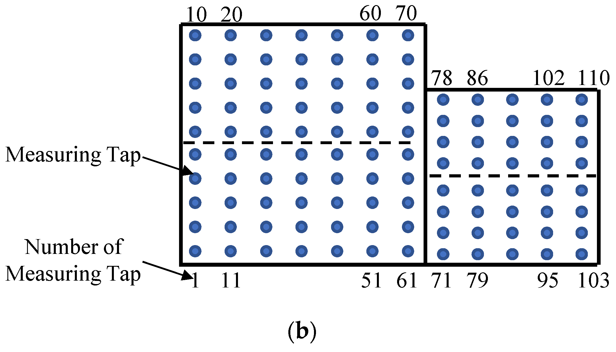
3.1. Test Model

The dimension of the tested specimen is demonstrated in Figure 3a. It is a 1:150 scale rigid model made of acrylonitrile butadiene styrene (ABS) plates. There are 110 measuring taps mounted on the surface of the model whose arrangement is plotted in Figure 3b. Every measuring tap is connected to PSI electronic pressure scanners through a 0.9 m length Polyvinyl chloride (PVC) tube. The errors caused by tube effects in pressure measurement results are modest and therefore neglected. Wind pressure histories for the model are recorded simultaneously.

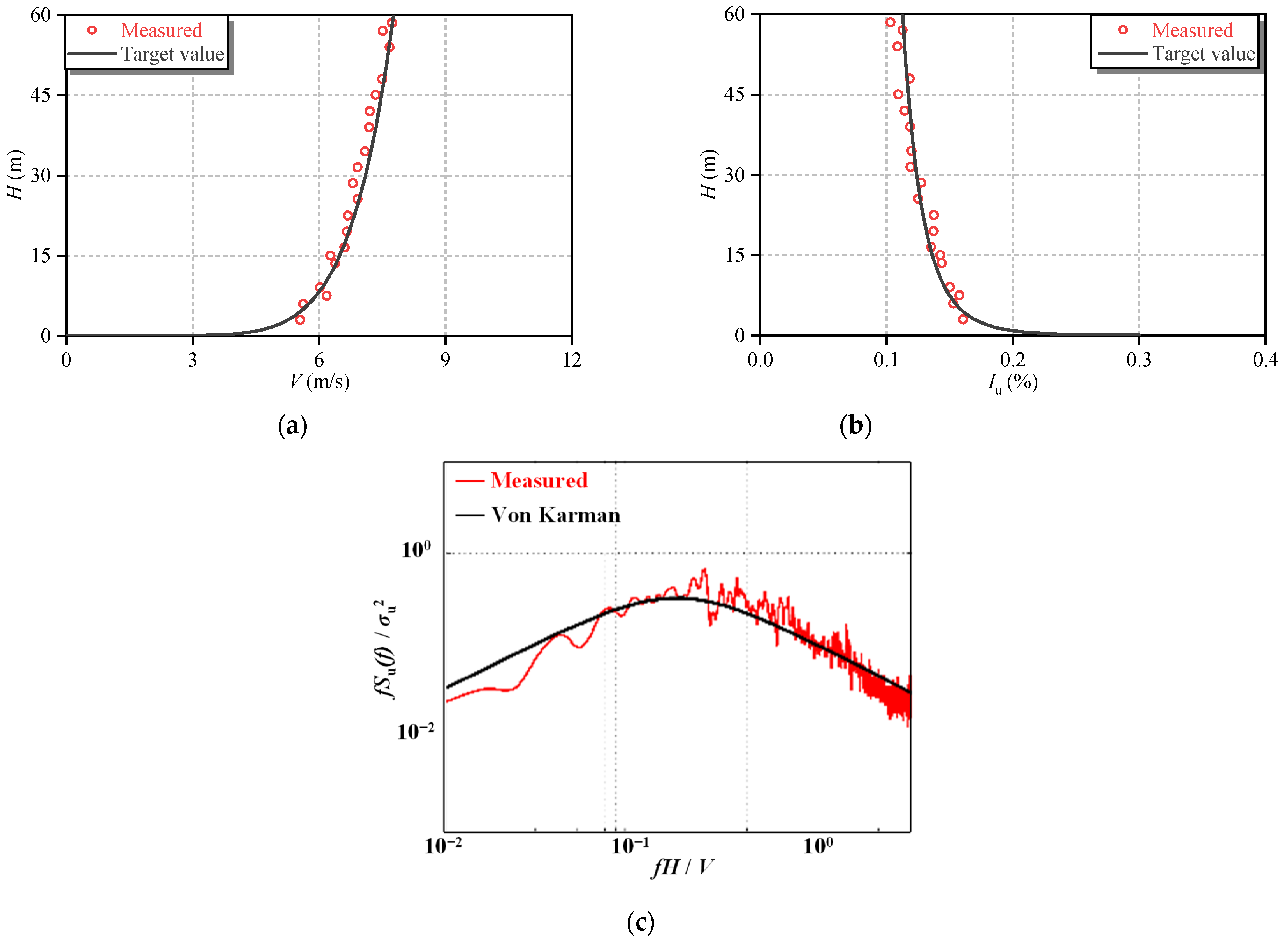
3.2. Wind Profile

Wind tunnel tests are conducted in an atmospheric boundary layer wind tunnel, whose testing sections are 3.0 m wide, 2.5 m tall, and 15.0 m long. The blockage ratio of the tested model is 4.9%, smaller than the critical value of 5%. The atmospheric boundary layer is simulated by setting roughness elements upstream of the testing section, as illustrated in Figure 4. The wind profile of terrain category B according to [5] is simulated in the wind tunnel test. The profiles of mean wind speed and turbulent intensity are:

$$V_H=V_0{\left(H/H_0\right)}^{\alpha }, \mathrm{and}$$

(21)

$$I_{\mathrm{H}}=I_{10}{\left(H/10\right)}^{-\alpha }.$$

(22)

Here, V_H and I_H refer to wind speed and turbulence intensity at height H. V₀ is the wind speed at the reference height H₀; I₁₀ = 0.14 is the nominal turbulence intensity at a height of 10 m for terrain category B; α = 0.15 is the exponential wind profile index for terrain category B.

The wind profiles in the freestream are investigated and the measured results are compared with target values including mean wind speed V and turbulence intensity I_u, which are plotted in Figure 5a,b. It can be observed that good agreement is achieved between the target and measured values. The power spectrum of measured wind speed at roof height is plotted in Figure 5c, which follows the Von Karman spectrum.

3.3. Wind Pressure Measurements

Wind pressures on the model surface are measured in 24 azimuths with an internal of 15°. As shown in Figure 4, the tested model is set at the center of the turntable. The variation of azimuths is realized by rotating the turntable. Under every azimuth, wind pressures of 110 taps are recorded simultaneously. The sampling frequency f_s is 312.5 Hz, and the sampling time t is 60 s. Following the assumption that a full-scale wind speed at 10 m height in suburban exposure is 25.3 m/s, the speed scale is derived as 1:2.5. The test wind speed is set at 10 m/s and the hot-wire anemometer is employed to measure the wind speed at the reference height. For a wind azimuth of 90°, the sampling time t is 1 h, corresponding to 60 h at full scale. The long-term data are divided into 360 segments of 10 min duration in the analysis of Section 5 to examine the validation of the HPM for calculation of the peak factors and extreme values of non-Gaussian wind pressures.

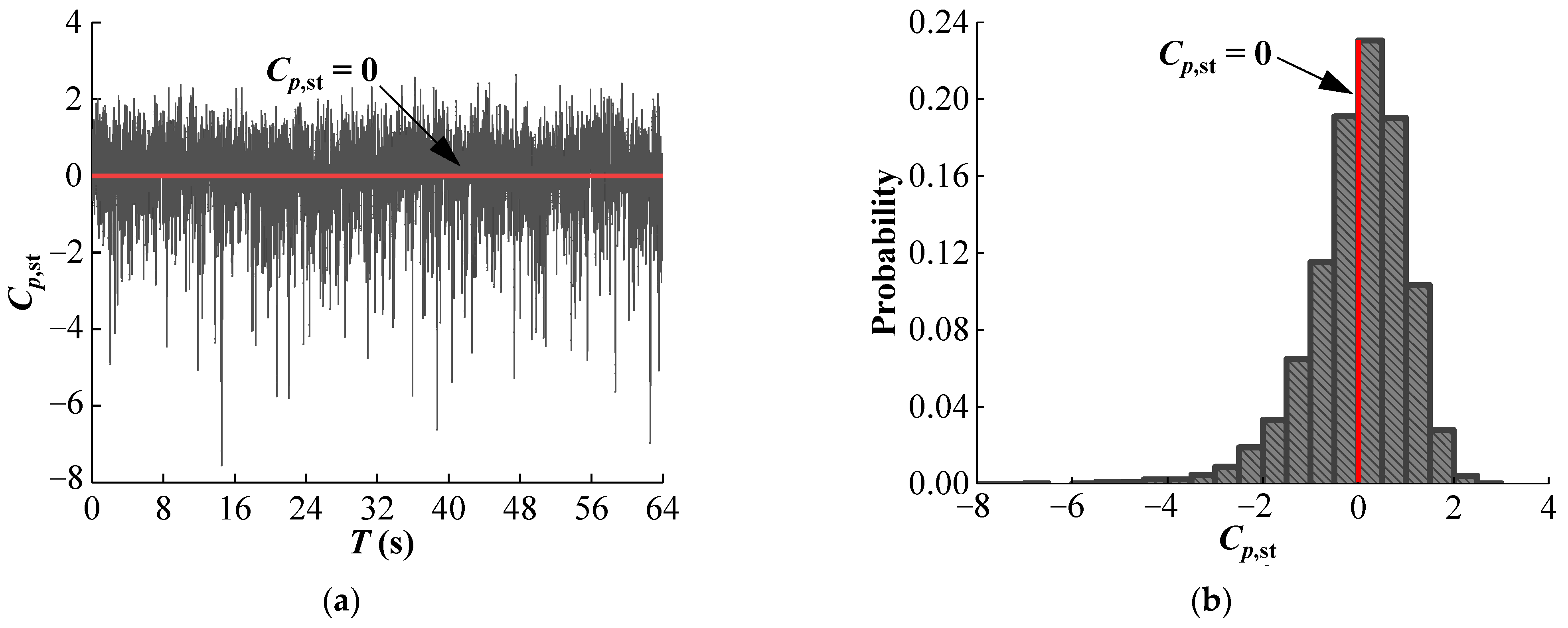
3.4. Data Processing of Wind Pressure

The measured wind pressure processes are converted to dimensionless pressure coefficients through:

$$C_{pi}\left(t_{\mathrm{m}}\right)=\frac{p_i\left(t_m\right)-p_{\infty }}{p_0-p_{\infty }},$$

(23)

where t_m = m/f_s, (m = 1, 2,…, N) is the time series, N = f_st = 312.5 × 60 = 18,750 is the sample length, p_i (t_m) refers to the measured wind pressure of tap i in the freestream, and p₀ and p_∞ are total pressure and static pressure at reference height in the freestream, respectively.

The mean and standard deviation values of wind pressure coefficients are obtained by:

$$C_{pi,\mathrm{mean}}=\frac{1}{N}{\displaystyle \sum _{m=1}^N{C}_{pi}}\left(t_m\right), \mathrm{and}$$

(24)

$$C_{pi,\mathrm{rms}}=\sqrt{\frac{1}{N-1}{{\displaystyle \sum _{m=1}^N\left[C_{pi}\left(t_m\right)-C_{pi,\mathrm{mean}}\right]}}^2}.$$

(25)

Then, the standardized pressure coefficient of tap i, C_pi,st (t_m) can be calculated by:

$$C_{pi,\mathrm{st}}\left(t_{\mathrm{m}}\right)=\left(C_{pi}\left(t_m\right)-C_{pi,\mathrm{mean}}\right)/C_{pi,\mathrm{rms}}.$$

(26)

It has been established that wind pressure characteristics are closely associated with structures’ configuration. Flow at the edge regions of the structures is fluctuant and should be paid more attention. Tap 66, situated at the right edge cd of BCR, is such a case where the wind flow is complex. As shown in Figure 6a, the pressure history for tap 66 is not symmetrical to the neutral axis where C_pi,st equals 0. Those intermittent negative impulses could lead to predominant suctions on the roof. As illustrated in Figure 6b, negative impulses have the precise effect of wind pressure being deviated from the Gaussian distribution and introducing a leftward long tail. Due to this, the suction on the roof is higher than for the Gaussian process though having the same first- and second-order moments.

4. Non-Gaussian Property of Wind Pressures

In this section, the non-Gaussian property of wind pressures is analyzed in terms of the statistical and spatial distribution for the mean value, skewness, and kurtosis of wind pressure. The sensitive regions with strong non-Gaussian properties are found.

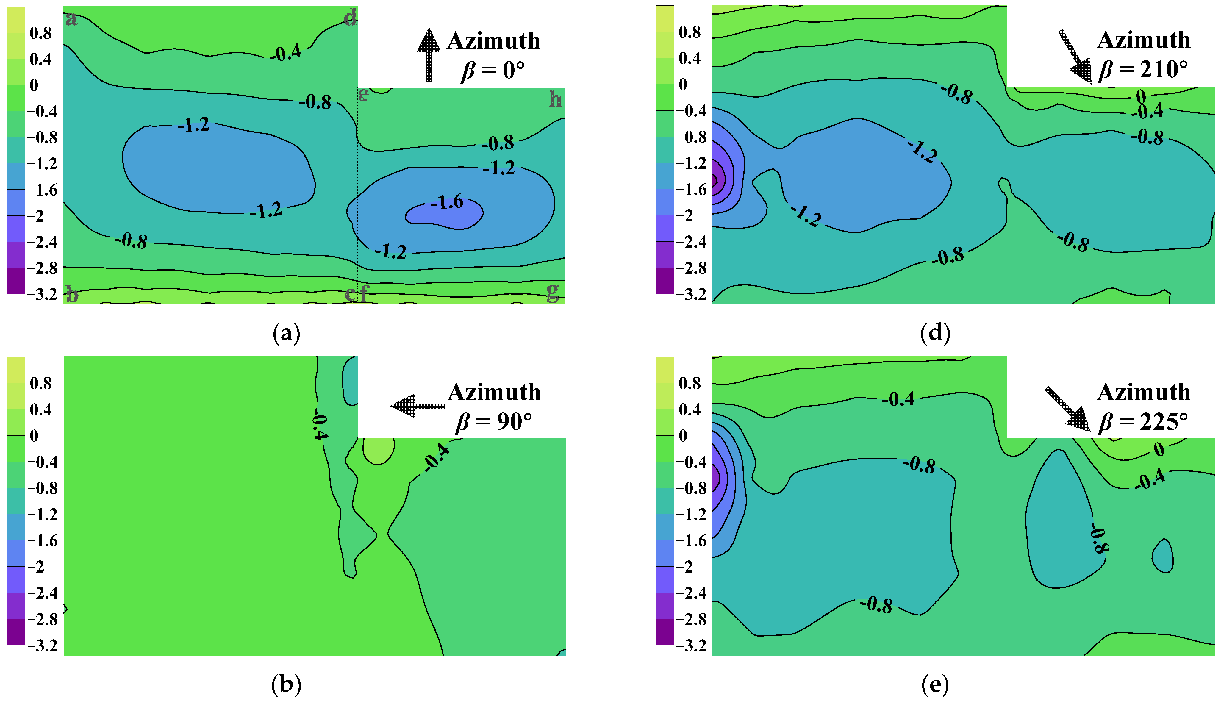
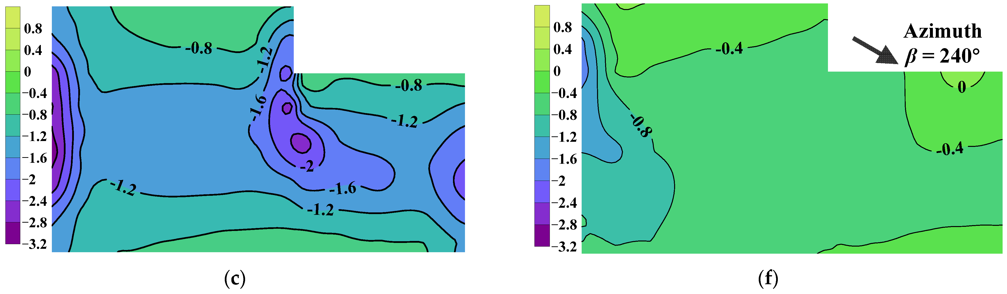
4.1. Mean Value of Wind Pressure

The sign of mean wind pressure coefficient, C_{p, mean}, is critical to identify whether the region is immersed in flow separation, where it is most likely to exhibit non-Gaussian properties. The experimental results of C_{p, mean} at five representative azimuths, i.e., β = 0°, 90°, 210°, 225°, and 240°, are presented in Figure 7. Contours are obtained using Surfer software. In comparison, the results of a single cylindrical roof presented in [30] are considered to illustrate the differences in wind pressure distribution characteristics between a combined cylindrical roof and a single one.

As shown in Figure 7a, the suction for BCR and SCR rooftops is considerable when the model is impacted by the windward flow, i.e., β = 0°. This is caused by the evident flow separation at the rooftops. Most of the C_{p, mean} are negative except those on the light green regions around windward edges bc and fg. This is because straightforward wind flow attacks the roof and air stagnation causes positive pressures. Such a wind pressure distribution is similar to that in [30] for a single cylindrical roof.

Figure 7b presents the spatial distribution of C_{p, mean} at β = 90°. The whole roof is dominated by negative pressures except for the region around the corner e. Because the blocked airflow around the BCR reverses its direction, the backflow dashes into the SCR roof, which eventually results in positive pressure. The wind flow separates at edges gh and cd, which leads to a dramatic reduction in wind energy. Therefore, the values of C_{p, mean} on the BCR are uniform and close to −0.3.

Figure 7d,f plots the distribution of the C_{p, mean} for β = 210°, 225°, and 240°. Most C_{p, mean} on the entire roof are negative while the positive coefficients are found in small regions, induced by the attachment of wind flow. It is noted that the wind pressure distribution on the SCR is impacted by the sheltering of the BCR. Therefore, the amplitude of wind pressure coefficients for the SCR is smaller than for the BCR.

The above finding indicates that most of the regions on the roof are immersed in flow separation, and the wind pressures on such regions tend to be non-Gaussian. By comparison, it can be concluded that the distribution of C_{p, mean} for the combined cylindrical roof is similar to that of the single one, only for β = 0°. The reserved results for the single cylindrical roof cannot be directly employed in the wind-resistant design of the combined cylindrical roof. Investigating the properties of the wind pressure on the combined cylindrical roof is essential.

The minimal mean wind pressure coefficients C_{p, mean, min} among all azimuths are investigated, whose distribution is shown in Figure 7c. It can be concluded that the entire roof is immersed in the flow separation given that all of the C_{p, mean, min} are negative. In addition, values of C_{p, mean, min} on edge ab and edge cd of the BCR and on edge ef of the SCR are much smaller, which indicates these parts have the largest mean wind suction. If the peak factors for these parts are predominant, the resulting extreme wind suction is considerable.

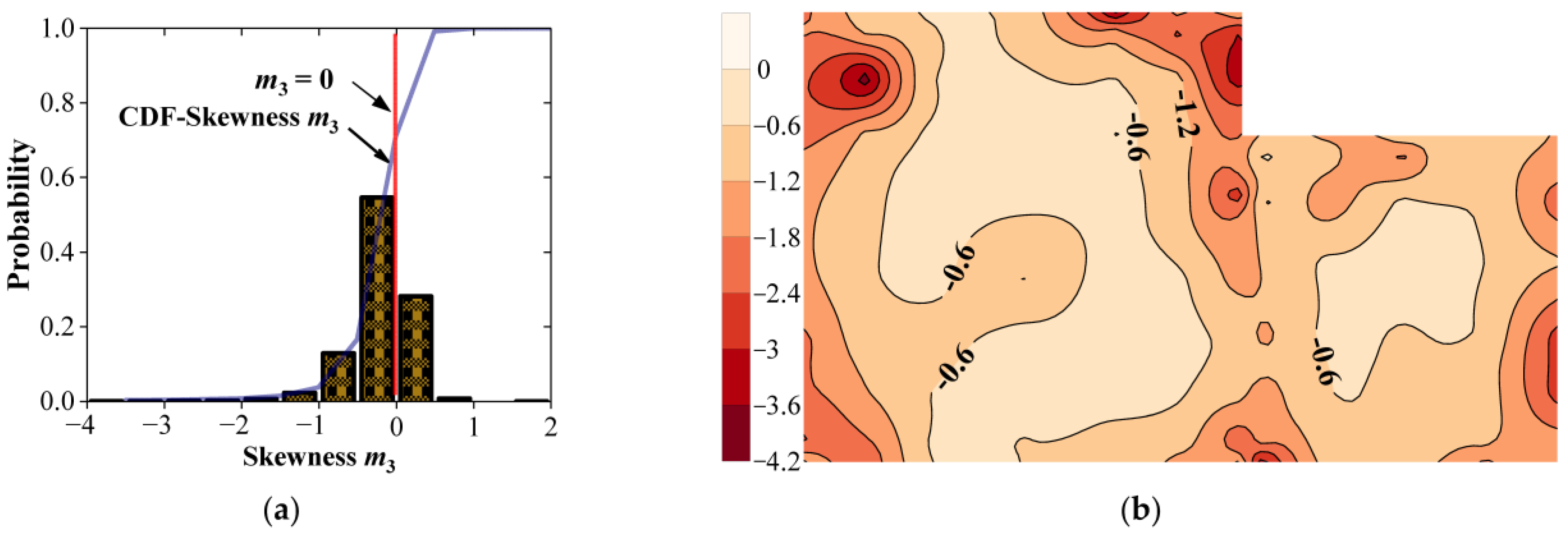
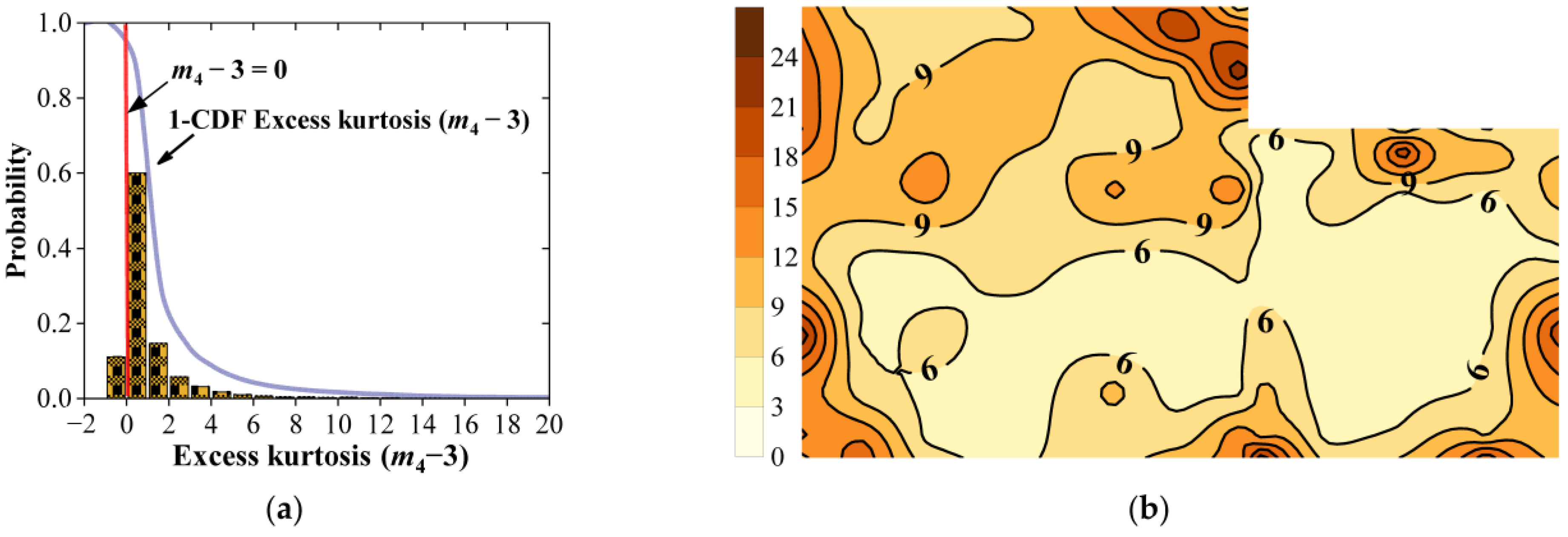
4.2. Skewness and Kurtosis of Wind Pressure

Skewness m₃ as well as kurtosis m₄ of wind pressure are calculated to identify whether the process is Gaussian. The definition of m₃ and m₄ for wind pressure coefficient C_pi is expressed as:

$$m_3=\frac{1}{N}{{\displaystyle \sum _{m=1}^N\left[\frac{C_{pi}(t_m)-C_{pi,\mathrm{mean}}}{C_{pi,\mathrm{rms}}}\right]}}^3, \mathrm{and}$$

(27)

$$m_4=\frac{1}{N}{{\displaystyle \sum _{m=1}^N\left[\frac{C_{pi}(t_m)-C_{pi,\mathrm{mean}}}{C_{pi,\mathrm{rms}}}\right]}}^4$$

(28)

The statistical and spatial distributions for wind pressure on the entire roof are examined. Statistical analysis is operated on wind pressure coefficient histories measured from 110 taps, including 24 wind azimuths. The histogram of skewness m₃ is presented in Figure 8a, in which the purple curve is the CDF of m₃. Most of the values for m₃ are distributed in the range [−1, 0], and 80% of them are smaller than −0.1. This indicates that most of the wind pressures are left-skewed regardless of azimuths. Moreover, roughly 18% of m₃ are smaller than −0.6, showing strong non-Gaussian properties.

The minimal value of m₃ for each tap among all tested wind azimuths is calculated. The spatial distribution of m_{3, min} is presented in Figure 8b. As can be seen, all m_{3, min} values are smaller than −0.3. The values of m_{3, min} for edge ab and edge cd of the BCR, as well as edge ef of the SCR, are less than −1.2. Moreover, values of m_{3, min} for corners a and d are even smaller than −2.0. The wind pressures for such regions are highly left-skewed. This is because flow separation and vortex shedding at curved edges and corners are distinct, resulting in evident non-Gaussian wind flow for those regions. Thus, wind pressures here exhibit a more predominant wind suction than that of a Gaussian distribution.

Figure 9a presents the histogram of excess kurtosis (m₄ − 3), in which the purple line is the exceedance probability of excess kurtosis, i.e., 1-CDF. Over 90% of (m₄ − 3) values are larger than 0. Roughly 17% of (m₄ − 3) values are larger than 1.0.

Furthermore, the maximal kurtosis m_{4, max} for every tap among all azimuths is calculated, whose distribution on the entire roof is shown in Figure 9b. All m_{4, max} values are larger than 3.5. This indicating the wind pressure history for each tap is the softening process. Moreover, the values of m_{4, max} around edge ab and edge cd of the BCR, as well as edge ef of the SCR, are more than 8.0, while corners a and d are even more than 13.0. All this suggests that the wind pressures on the long-span roof have more outliers than the Gaussian distribution and are leptokurtic. Therefore, extreme wind pressures are deemed to be considerable. Still, using the Gaussian assumption will underestimate extreme suction in the sensitive regions.

5. Peak Factors and Extreme Values of Wind Pressure

The peak factor for each tap is calculated by averaging the largest values selected from each of the 360 segments of the normalized wind pressure coefficient data of β = 90°. As shown in Figure 10, test results are compared with the determination via the HPM given in Section 2, i.e., Equation (15). It is observed that the HPM provides excellent estimations for most wind pressures, with a relative error of no more than 5%. Hence, the HPM is employed to determine peak factors in this study.

The distribution of peak factors for three representative wind azimuths, β = 210°, 225°, and 240°, is shown in Figure 11a–c, respectively. Peak factors are all larger than 3.5. Furthermore, every contour has a small region with peak factors even larger than 8.5. As presented in Figure 12a, the histogram is the peak factors for all measurements, in which the purple line is the exceedance probability of peak factors. About 60% of them are larger than 5.0, and 20% exceed 7.0.

The histogram of maximal peak factor g_{peak, max} is presented in Figure 12b, in which all the g_{peak, max} values are larger than 5.5, and even 60% of them are larger than 9.0. It can be concluded that peak factors for such roofs are much more considerable than 2.5 and others following the Gaussian assumption. Additionally, the spatial distribution of g_{peak, max} is presented in Figure 11d. Peak factors are predominant around edge ab and edge cd of the BCR as well as edge ef of the SCR. As presented in Figure 7c, C_{p, mean, min} also exhibit their minimums around these regions which are deemed to have predominant wind suctions and be the most sensitive.

For the wind-resistant design of the roof, extreme wind pressures are important parameters. Accordingly, the influence of the non-Gaussian property on the extreme wind pressures is investigated hereafter. Considering that most of the mean values of wind pressure coefficients are negative, only negative extreme wind pressures are included. As shown in

Table 1. Extreme wind pressures of taps based on g_{peak, max}.

Tap	β	Cp,mean	Cp,rms	gpeak, NG	gpeak, G	1 Cp, peak, NG	2 Cp, peak, G	3 Cp, peak, 2.5	2/1	3/1
5	255	−1.01	0.10	10.87	4.01	−2.12	−1.42	−1.27	0.67	0.60
7	285	−0.81	0.12	14.08	4.05	−2.47	−1.29	−1.11	0.52	0.45
69	345	−0.37	0.13	10.05	3.92	−1.72	−0.90	−0.70	0.52	0.41
72	225	−0.52	0.14	10.95	3.96	−2.00	−1.06	−0.86	0.53	0.43
104	210	−0.61	0.21	10.15	3.99	−2.75	−1.45	−1.13	0.53	0.41
109	330	−0.56	0.20	10.11	3.98	−2.59	−1.36	−1.06	0.52	0.41

, the extreme wind pressure coefficients for six taps are collected based on g_{peak, max}. For comparison, peak factors g_{peak, G}, following Gaussian assumption, and a constant peak factor of 2.5 are also considered for extreme wind pressure calculation, namely C_{p, peak, G} and C_{p, peak, 2.5}.

According to Table 1, g_{peak, NG} is about three times g_{peak, G}, leading to the discrepancy between C_{p, peak, NG} and C_{p, peak, G} being significant. The influence of the non-Gaussian property on the resulting extreme wind pressure is considerable. Therefore, the use of g_{peak, G,} or 2.5 is not suitable for the calculation of extreme wind pressures on the combined long-span cylindrical roofs. Generally, the envelope of wind pressure coefficients among all azimuths is important for designers. However, the maximum g_peak does not always indicate the maximum extreme wind pressure. Thus, the influence of the non-Gaussian property on the maximums of wind pressure coefficients among all azimuths is also investigated.

The wind pressure coefficients when the extreme value at each tap is maximum among the tested azimuths, i.e., C_{p, peak, max}, are listed in

Table 2. Extreme wind pressures of taps based on C_{p, peak, max}.

Tap	β	Cp, mean	Cp,rms	gpeak, NG	gpeak, G	1 Cp, peak, NG	2 Cp, peak, G	3 Cp, peak, 2.5	2/1	3/1
5	225	−1.73	0.35	8.34	3.94	−4.66	−3.11	−2.61	0.67	0.56
7	240	−1.91	0.39	8.62	4.03	−5.29	−3.49	−2.89	0.66	0.55
69	90	−0.94	0.30	5.79	3.96	−2.71	−2.15	−1.71	0.79	0.63
72	210	−0.57	0.21	9.85	3.94	−2.64	−1.40	−1.09	0.53	0.41
104	210	−0.61	0.21	10.15	3.99	−2.75	−1.45	−1.13	0.53	0.41
109	330	−0.56	0.20	10.11	3.98	−2.59	−1.36	−1.06	0.52	0.41

. The difference between C_{p, peak} and C_{p, peak, G} is dramatic, as well as C_{p, peak} and C_{p, peak, 2.5}. Extreme wind pressures are underestimated due to ignoring non-Gaussian properties of wind pressure. As for the taps listed in Table 2, the determination for C_{p, peak, 2.5} is only 50% of C_{p, peak, NG} while C_{p, peak, G} accounts for 60% of C_{p, peak, NG}. It can be concluded that neglecting the non-Gaussian property will underestimate extreme wind pressure on the combined long-span cylindrical roof by 40–50%. Therefore, the non-Gaussian property of wind pressure must be included when estimating extreme wind pressures on the combined long-span cylindrical roof. Still, following the present method in the Chinese standard will result in significant underestimates of extreme wind pressures in the sensitive regions, and the structural design would be unsafe.

6. Conclusions

The non-Gaussian property and its influence on extreme wind pressures on the combined long-span cylindrical roof are systemically investigated in this study. The sensitive regions that exhibit strong non-Gaussian properties are found. The main findings are as follows:

(1)

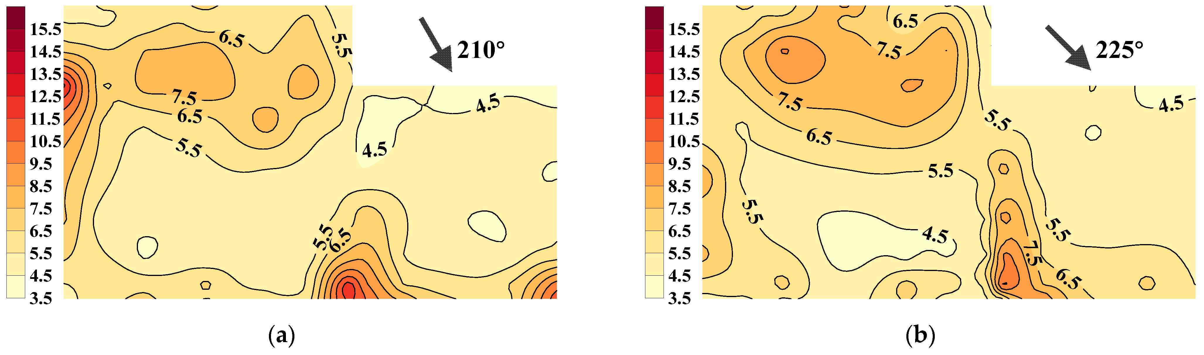
Wind tunnel test results indicate that wind pressures on the combined cylindrical roof are left-skewed softening processes when the worst case among all tested wind azimuths is considered. Regions around curved edges along the span of the cylindrical roof are revealed as having strong non-Gaussian properties.

(2)

The HPM is verified by wind tunnel test results being capable of calculating peak factors and extreme values of non-Gaussian wind pressures on the combined cylindrical roof with a relative error of no more than 5%.

(3)

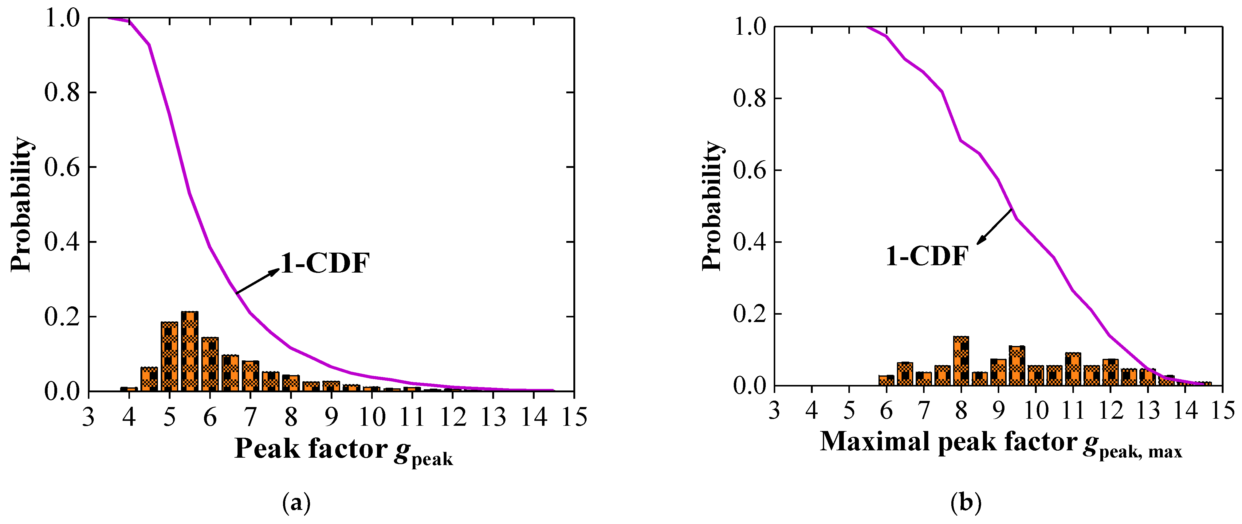
All the maximal peak factors are larger than 5.0, and 20% of them are even larger than 7.0. Using peak factors following the Gaussian assumption or 2.5 underestimates the extreme values of wind pressures by 40–50%.

(4)

It is necessary to include the non-Gaussian properties when estimating the extreme values of wind pressure on such long-span cylindrical roofs in engineering practice.

It is noted that the results presented in this paper are preliminary based on the wind tunnel test results for the scaled model of the roof. Therefore, further work is needed to create a full-scale model of the L-shaped long-span cylindrical roof and investigate it numerically.

References

- ASCE/SEI 7-22; American Standard: Minimum Design Loads and Associated Criteria for Buildings and Other Structures. American Society of Civil Engineers Press: Reston, VA, America, 2022.
- AS/NZS 1170.2:2021; Australian/New Zealand Standard: Structural design actions—Part 2: Wind actions. Council of Standards Australia Press: Australia/New Zealand, 2021.
- AIJ-RLB; Japanese Standard: Recommendations for Loads on Buildings. Structural Standards Committee Press: Tokyo, Japan, 2015.
- NR24-28/2020E; Canadian Standard: National Building Code. Associate Committee on the National Research Council Press: Ottawa, ON, Canada, 2020.
- GB 50009-2019; Chinese Standard: Load Code for the Design of Building Structures. National Standards Committee Press: Beijing, China, 2019.
- Cope, A.D.; Gurley, K.R.; Gioffre, M.; Reinhold, T.A. Low-rise gable roof wind loads: Characterization and stochastic simulation. J. Wind. Eng. Ind. Aerod 2005, 93, 719–738. [Google Scholar] [CrossRef]
- Kumar, K.S.; Stathopoulos, T. Synthesis of non-Gaussian wind pressure time series on low building roofs. Eng. Struct. 1999, 21, 1086–1100. [Google Scholar] [CrossRef]
- Kwon, D.K.; Kareem, A. Peak factors for non-Gaussian load effects revisited. J. Struct. Eng. 2011, 137, 1611–1619. [Google Scholar] [CrossRef]
- Wang, D.Z.; Zhi, X.D.; Fan, F.; Lin, L. The energy-based failure mechanism of reticulated domes subjected to impact. Thin-Walled Struct. 2017, 119, 356–370. [Google Scholar] [CrossRef]
- Zhang, J.; Zhu, B.Y.; Wang, F.; Tang, W.X.; Wang, W.B.; Zhang, M. Buckling of prolate egg-shaped domes under hydrostatic external pressure. Thin-Walled Struct. 2017, 119, 296–303. [Google Scholar] [CrossRef]
- Balderrama, J.A.; Masters, F.J.; Gurley, K.R. Peak factor estimation in hurricane surface winds. J. Wind. Eng. Ind. Aerod 2012, 102, 1–13. [Google Scholar] [CrossRef]
- Yang, Q.S.; Tian, Y.J. A model of probability density function of non-Gaussian wind pressure with multiple samples. J. Wind. Eng. Ind. Aerod 2015, 140, 67–78. [Google Scholar] [CrossRef]
- Kasperski, M. Specification of the design wind load-A critical review of code concepts. J. Wind. Eng. Ind. Aerod 2009, 97, 335–357. [Google Scholar] [CrossRef]
- Kasperski, M. Specification of the design wind load based on wind tunnel experiments. J. Wind. Eng. Ind. Aerod 2003, 91, 527–541. [Google Scholar] [CrossRef]
- Holmes, J.D.; Cochran, L.S. Probability distributions of extreme pressure coefficients. J. Wind. Eng. Ind. Aerod 2003, 91, 893–901. [Google Scholar] [CrossRef]
- Yang, L.P.; Gurley, K.R.; Prevatt, D.O. Probabilistic modeling of wind pressure on low-rise buildings. J. Wind. Eng. Ind. Aerod 2013, 114, 18–26. [Google Scholar] [CrossRef]
- Peng, X.L.; Yang, L.P.; Gavanski, E.; Gurley, K.; Prevatt, D. A comparison of methods to estimate peak wind loads on buildings. J. Wind. Eng. Ind. Aerod 2014, 126, 11–23. [Google Scholar] [CrossRef]
- Ding, J.; Chen, X.Z. Assessment of methods for extreme value analysis of non-Gaussian wind effects with short-term time history samples. Eng. Struct. 2014, 80, 75–88. [Google Scholar] [CrossRef]
- Gioffre, M.; Gusella, V.; Grigoriu, M. Non-Gaussian wind pressure on prismatic buildings. I: Stochastic field. J. Struct. Eng. 2001, 127, 981–989. [Google Scholar] [CrossRef]
- Chen, X.Z.; Huang, G.P. Evaluation of peak resultant response for wind-excited tall buildings. Eng. Struct. 2009, 31, 858–868. [Google Scholar] [CrossRef]
- Cluni, F.; Gusella, V.; Spence, S.M.J.; Bartoli, G. Wind action on regular and irregular tall buildings: Higher order moment statistical analysis by HFFB and SMPSS measurements. J. Wind. Eng. Ind. Aerod 2011, 99, 682–690. [Google Scholar] [CrossRef]
- Huang, M.F.; Lou, W.; Chan, C.M.; Lin, N.; Pan, X. Peak factors of non-Gaussian wind forces on a complex-shaped tall building. Struct. Des. Tall Special Build. 2013, 22, 1105–1118. [Google Scholar] [CrossRef]
- Ma, X.L.; Xu, F.Y. Peak factor estimation of non-Gaussian wind pressure on high-rise buildings. Struct. Des. Tall Special Build. 2017, 26, e1386. [Google Scholar] [CrossRef]
- Ayed, S.B.; Aponte-Bermudez, L.D.; Hajj, M.; Tieleman, H.W.; Gurley, K.R.; Reinhold, T.A. Analysis of hurricane wind loads on low-rise structures. Eng. Struct. 2011, 33, 3590–3596. [Google Scholar] [CrossRef]
- Huang, G.Q.; He, H.; Mehta, K.C.; Liu, X.B. Data-based probabilistic damage estimation for asphalt shingle roofing. J. Struct. Eng. 2015, 141, 04015065. [Google Scholar] [CrossRef]
- Gavanski, E.; Gurley, K.R.; Kopp, G.A. Uncertainties in the estimation of local peak pressures on low-rise buildings by using the Gumbel distribution fitting approach. J. Struct. Eng. 2016, 142, 04016106. [Google Scholar] [CrossRef]
- Zhao, H.; Grigoriu, M.; Gurley, K.R. Translation processes for wind pressures on low-rise buildings. J. Wind. Eng. Ind. Aerod 2019, 184, 405–416. [Google Scholar] [CrossRef]
- Song, J.; Xu, W.; Hu, G.; Liang, S.; Tan, J. Non-Gaussian properties and their effects on extreme values of wind pressure on the roof of long-span structures. J. Wind. Eng. Ind. Aerod 2019, 184, 106–115. [Google Scholar] [CrossRef]
- Li, T.; Yang, Q.S.; Ishihara, T. Unsteady aerodynamic characteristics of long-span roofs under forced excitation. J. Wind. Eng. Ind. Aerod 2018, 181, 46–60. [Google Scholar] [CrossRef]
- Li, Y.Q.; Tamura, Y.; Yoshida, A.; Katsumura, A.; Cho, K. Wind loading and its effects on single-layer reticulated cylindrical shells. J. Wind. Eng. Ind. Aerod 2006, 94, 949–973. [Google Scholar] [CrossRef]
- Winterstein, S.R.; Kashef, T. Moment-based load and response models with wind engineering applications. J. Sol. Energy Eng. 2000, 122, 122–128. [Google Scholar] [CrossRef]