


Fault Diagnosis Method of Rolling Bearing Based on CBAM_ResNet and ACON Activation Function

1
Key Laboratory of Advanced Manufacturing and Automation Technology (Guilin University of Technology), Education Department of Guangxi Zhuang Autonomous Region, Guilin 541006, China
2
Guangxi Engineering Research Center of Intelligent Rubber Equipment (Guilin University of Technology), Guilin 541006, China
*
Author to whom correspondence should be addressed.
Appl. Sci. 2023, 13(13), 7593; https://doi.org/10.3390/app13137593
Submission received: 29 May 2023
/
Revised: 22 June 2023
/
Accepted: 26 June 2023
/
Published: 27 June 2023
(This article belongs to the Special Issue Fault Diagnosis and Detection of Machinery)
Abstract
:In order to cope with the influences of noise interference and variable load on rolling bearing fault diagnosis in real industrial environments, a rolling bearing fault diagnosis method based on CBAM_ResNet and ACON activation function is proposed. Firstly, the collected bearing working vibration signals are made into input samples to retain the original features to the maximum extent. Secondly, the CBAM_ResNet fault diagnosis model is constructed. By taking advantage of the convolutional neural network (CNN) in classification tasks and key feature extraction, the convolutional block attention module network (CBAM) is embedded in the residual blocks, to avoid model degradation and enhance the interaction of information in channel and spatial, raise the key feature extraction capability of the model. Finally, the Activate or Not (ACON) activation function, is introduced to adaptively activate shallow features for the purpose of improving the model’s feature representation and generalization capability. The bearing dataset of Case Western Reserve University (CWRU) is used for experiments, and the average accuracy of the proposed method is 97.68% and 93.93% under strong noise interference and variable load, respectively. Compared with the other three published bearing fault diagnosis methods, the results indicate that this proposed method has better noise immunity and generalization ability, and has good application value.
1. Introduction
Rolling bearings, as essential parts of machinery, are widely used in various industries [1]. The faults of rolling bearings in rotating machinery and equipment may cause production stoppage or even major accidents [2], so it is especially important to monitor and diagnose the operating condition of rolling bearings. Monitoring based on vibration signals is not affected by the mechanical structure and is simple to test, so it is one of the widely studied and applied fault diagnosis techniques [3]. By using the collected rolling bearing’s operating vibration signal data, the research of efficient and feasible fault diagnosis method, is of great significance to the timely detection of faults and normal works of mechanical equipment, which also is the motivation for our study.
In recent years, with the purpose of relying on vibration data for fault diagnosis, data-driven intelligent fault diagnosis techniques have been developed tremendously [4]. According to extensive reports, two keys to fault diagnosis are feature extraction and fault classification [5]. For instance, H.Habbouche et al. [6] used variational modal decomposition (VMD) for fault feature detection, then by virtue of convolution-pooling structures to trigger multi-scale features for diagnosis, experimental results validated that their method has good applicability in rolling bearing fault diagnosis. Jaouher B.A et al. [7] used empirical modal decomposition (EMD) to search the features of signals to choose the paramount intrinsic mode function (IMF) and finally combined it with an artificial neural network (ANN) for fault diagnosis of rolling bearings. Hou et al. [8] used wavelet transform (WT) to decompose the signal at multiple scales, and then input it to the constructed 1DCNN to obtain very high results for rolling bearing fault diagnosis. The above studies have a similar process, that is, they first extracted features in the vibration signal with the help of different signal processing methods, then input features to a shallow neural network for diagnostic classification. This process is known as machine learning applied to fault diagnosis [9,10,11]. These studies have promoted the development of the field of rolling bearing fault diagnosis, but there are problems of high manual feature extraction workload, heavy reliance on expert experience and knowledge, and strong subjective factors.
Deep learning fault diagnosis methods without relying on expert experience, can directly extract important features from vibration signals, which is difficult to achieve by using traditional machine learning [12]. Convolutional neural networks are very effective network structures in deep learning, and therefore, many scholars have used them for fault diagnosis. Saucedo-Dorantes et al. [13] proposed a novel data-driven diagnosis method based on deep feature learning for fault diagnosis of bearings with different advanced material processes such as metal bearings, hybrid ceramic bearings, and ceramic bearings. Yang et al. [14] used adversarial neural networks (GAN) to generate two-dimensional grayscale images of faulty vibration signals, which were combined with two-dimensional CNN (2DCNN) to complete the fault diagnosis of bearings. Wen et al. [15] proposed a novel CNN model similar to the LeNet-5 structure, which can extract the features of transformed 2D images and eliminate the influence of manually extracted features, and the method is verified to have good fault diagnosis results. Although these methods achieve good fault diagnosis results without the intervention of expert experience, however, in reality, machinery and equipment often work in an environment of intermingled noise, high speed, and variable load, on the one hand, the noise will greatly interfere with the effective information in the vibration signal, on the other hand, high-speed variable load significantly increases the complexity and uncertainty of the vibration signal.
Affected by noise interference and variable loads, deep learning fault diagnosis methods perform unstably in extracting fault features [16], and subsequently, the accuracy decreases and the generalization deteriorates, which eventually makes fault diagnosis challenging. Therefore, based on such considerations, some scholars have studied deep learning methods of response. Cao et al. [17] used kernels of different sizes in the first part of the model to construct a multi-scale 1DCNN that can capture fault features at different resolutions and enable fault diagnosis and simulated a noisy environment for diagnosis. Zhang et al. [18] proposed a domain-adaptive rolling bearing fault diagnosis model, called WDCNN, which has the significant advantage of resisting noise interference from vibration signals by using a wider convolutional kernel size in the first layer of the CNN and can be applied in the case of load variations. Liu et al. [19] proposed a multi-task 1DCNN, to improve fault diagnosis performance using two auxiliary tasks: speed identification task (SIT) and load identification task (LIT). Zhang [20] et al. proposed a CNN with training interference (TICNN), which achieves higher accuracy in noise and can be tested under different load conditions. These methods are designed to cope with the effects of realistic environments for fault diagnosis, but it is still room for improvement in these methods. What has been demonstrated is that CNNs are sensitive to other information about the real environment, such as noise and changing load conditions [21]. It can be improved by using one of its variants, the residual network, similar to what Ref [22,23] did, which focuses on improving the noise-resistant performance of CNN by increasing the number of layers with the help of residual connections, verifies that this technique is efficient when applied to fault diagnosis, unfortunately, however, they do not further explore the effect of variable load. Furthermore, using novel activation functions or attention mechanisms can help CNN to obtain better performance [24]. Such as in [12,25,26,27,28], more or less, they seek or design suitable novel techniques to apply to their methods and enhance the performance for fault diagnosis.
In a general overview, we found three problems with the vibration signal-based fault diagnosis method:
First, traditional machine learning applications for fault diagnosis emphasize the use of signal processing to extract important features and then input them into a shallow fault classifier. This relies heavily on expert experience.
Second, deep learning fault diagnosis methods do not emphasize expert experience but still need to further consider the impact of a realistic environment on it, such as noise and variable load.
Third, CNN, as an excellent representative of deep learning, is unsatisfactory when applied to fault diagnosis considering realistic environments, and it is necessary to adopt techniques such as using residual connections to deepen the network and adding attention mechanisms to counteract useless information.
Hence, we designed a coping method based on CBAM_ResNet and ACON activation functions. The main contributes of this paper are:
- (1)
- A novel CNN named CBAM_ResNet is proposed and the ACON activation function is used in it. Our method does not rely on expert experience for fault diagnosis, it achieves 100% diagnosis of the experimental data.
- (2)
- The effects of realistic environments such as noise and load variations on our method are considered, and compared with other publicly available fault diagnosis methods in the same consideration, our method performs better.
- (3)
- By employing two optimization techniques: embedding the CBAM attention mechanism into the residual block and introducing the ACON activation function, the performance of fault diagnosis is improved, which maintains high diagnostic accuracy under noise interference and has the ability to generalize to cope with load variations.
The rest of this paper can be summarized as follows: Section 2 presents the materials and methods used to construct the proposed model. The specific framework structure and parameters of the proposed model are also given in Section 2. Section 3 verifies the performance of the proposed model through several experiments and a discussion of the ablation experiments. Section 4 concludes the whole paper and presents our future research focus.
2. Materials and Methods
2.1. CNN
Convolutional neural networks (CNN) contain a two-stage structure of convolution and classification [29]. The convolutional structure mainly uses convolutional layers to learn features from the input layer data, pooling layers are connected after the convolutional layer to accelerate learning, and the classification structure mainly contains fully connected layers and output layers. The basic structure of a typical CNN is shown in Figure 1.
2.1.1. Convolution Layer
The operation of the convolution layer is the core of CNN, which extracts the local features in the input data, and its computational principle is shown in Equation (1):
where is an arbitrary activation function, is the convolution calculation, is the number of layers, l-layer interior, is the eigenvalue, is the convolution kernel, is the bias term, and is the output eigenvalue.
2.1.2. Pooling Layer
The use of pooling in fault diagnosis can filter out irrelevant information [30]. The operation of the pooling layer changes the dimensionality of the features, reducing the complexity of the model, while speeding up the operation and alleviating overfitting, the principle of pooling calculation is shown in Equation (2):
where is the output after pooling, is the pooling range, and is the coordinate of the pooling location.
2.1.3. ReLU Activation Function
The ReLU has become the default activation function for many types of neural networks because the models using it are easier to train. Unless otherwise stated, the activation functions in this paper will use ReLU.
2.1.4. Fully Connected Layer
In neural networks working on classification, the fully connected layer (FC) has a crucial role. The layer before FC is to extract features, and the role of FC is to classify the features. However, too many parameters of the FC will lead the model to be too redundant. In this paper, we use adaptive average pooling (AAP) to compress the features and then access the FC to output the classified results.
2.2. Residual Network
Residual networks [31] incorporate residual learning in serial convolutional layers. This network has obvious hierarchical relationships, eliminates the problem of difficult training of networks with too large depths, ensures the output feature expressiveness and this structure of introducing constant mapping fundamentally solves the gradient disappearance and degradation, only the difference between the input and the output is learned. The structure of the residual block is shown in Figure 2.
2.3. ACON Activation Function
The family of ACON activation functions was proposed by Ma Ningning [32] in 2021, in which the Meta ACON-C activation function adaptively decides whether a neuron is activated or not to help improve the transmission performance and the generalization performance of the network, which can improve the phenomenon of “neuron necrosis” to a certain extent and suppress the redundant information in the collected vibration signals. The principle of the family of ACON activation functions is to make an approximate smoothing of a standard maximum function, as shown in Equation (4):
where is the input feature vector, is the number of samples, and is the switching factor. If it is desired that the entire smoothing activation function behaves as a complete nonlinear activation, is required, at which point approximates the maximum value; instead, it behaves as a linear average then it does not activate, is required, at which point approximates the average value.
2.3.1. ACON-C
The family of ACON activation functions mainly includes three subclasses with different suffixes A, B, and C. The proposer verified that the subclass ACON-C is relatively better, and its principle is shown in Equation (5):
where is the Sigmoid activation function, , are two linear functions with slopes less than 1 and different, is the difference between the slopes of the linear functions, and the range of first-order derivatives of ACON-C can be determined by controlling .
2.3.2. Meta ACON-C
The Meta ACON-C activation function can accomplish adaptive switching between linear and nonlinear mapping by iteratively defining the switching factor. It can be obtained by making modifications on the basis of AOCN-C. Referring to the modification methods in the image field [33], a multi-channel one-dimensional adaptive function based channel-wise is designed as shown in Equation (6) to obtain the one-dimensional Meta ACON-C activation function that is used in this paper.
where is the value of the adaptive function of the input sample data channel, which can be obtained by assigning the same weight to the same element across channels by the switching factor, is the Sigmoid activation function, and are the sample dimension dimensions, , , is the scaling factor, which is usually taken to the power of 2.
2.4. CBAM
The attention mechanism borrows the way of resource allocation in human perceptual behavior, and its ability to give more attention to important information to achieve the purpose of obtaining more detailed information in the target task [34]. Among them, the Convolutional Block Attention Module (CBAM) is widely used in deep learning networks due to its fewer parameters, higher speed, and higher flexibility, and has been proved that the network model learns more important features when it is applied. The CBAM is structured in such a way that the channel attention module is directly in series with the spatial attention module, as shown in Figure 3.
2.4.1. Channel Attention Module
This module is characterized by constant channel dimension and compressing spatial dimension, focusing on the “why” of the sample divided into different categories. The calculation process of the channel attention module is shown in Equation (7):
where is the feature matrix with fused channel attention weights, is the channel attention weights, is the average pooling operation, is the maximum pooling operation, is the multilayer perceptron (MLP), and is the Sigmoid activation function.
2.4.2. Spatial Attention Module
In contrast to the former, this module is characterized by maintaining spatial dimension and compressing channel dimension. What distinguishes the spatial attention module from the former is it more concerned with “where” the information is. The calculation process of the spatial attention module is shown in Equation (8):
where is the feature matrix incorporating the spatial attention weights, is the channel attention weights, and is the convolution operation, in this paper kernel size of the spatial attention module is 3.
2.5. Proposed Methodology
Fault diagnosis is actually inseparable from the classification task. CNN has obvious advantages in classification tasks and key feature extraction. However, on the one hand, traditional CNN extracts deeper features by deepening the number of network layers. Unfortunately, when the number of layers is too large, the network model faces the problem of gradient dispersion or explosion and network degradation [35], which will lead to a decrease in the accuracy of fault diagnosis models.
On the other hand, in actual industrial production, the vibration signal is highly susceptible to interference from environmental noise, and the transforming load work increases the complexity of the collected data, thus, weakening the ability of the model to extract key features. To cope with these problems, this paper constructs a CNN with residual connections while combining the CBAM attention mechanism and ACON activation function, and proposes a rolling bearing fault diagnosis model based on CBAM_ResNet and ACON activation function.
2.5.1. Proposed Model
The proposed model mainly consists of a convolutional layer, maximum pooling layer, improved residual block, AAP layer, and FC layer. The network structure of the proposed model is shown in Figure 4.
Residual networks deepen the number of network layers through residual learning to obtain deep features [31,35]. In this paper, we use modified residual blocks to extract deeper features for fault diagnosis.
The construction of a suitable first feature extraction layer in CNN plays a vital role in the performance of the whole model [18,20,30]. In this paper, we use a wider convolutional kernel to enhance the perceptual field in the first layer of the model to reduce the influence of noise on the model feature extraction in a small area and provide assurance for the subsequent extraction of deeper key features.
By dynamically learning the parameters of the ACON activation function and designing different forms of activation for each neuron, the feature representation capability of the model can be improved, thus making the model more generalizable [36]. In this paper, a convolutional layer based on the meta ACON-C activation function is designed between a wide kernel convolutional layer and an improved residual block. After extracting local features, it is used to improve the generalization performance of the model by exploiting the adaptive activation properties of the ACON activation function.
CBAM, as an attention mechanism, captures both channel features and spatial features, and has good embeddable ability [37], which first achieves control of global information by establishing the connection between feature channels and then finding important information in the channel axis space to enhance the sensitivity of the model to key features, raises the model performance. In this paper, CBAM is embedded into the residual blocks to obtain more feature information on channels and spaces within the residual connections by improving the blocks of the residual network. The CBAM_ResNet is constructed, and the model has deep key feature extraction ability, which can effectively suppress redundant information interference and solve the problems of gradient dispersion and network degradation at the same time.
2.5.2. Improved Residual Block
In the improved residual block, the input feature x is first calculated by two 3 × 1 convolutions to obtain the feature F(x), which then enters CBAM to calculate the weights of the channel and spatial information. Next, the weights obtained are dotted with F(x), and finally summed with x to obtain G(x). The structure of the improved residual block is shown in Figure 5.
The 1 × 1 convolution of the dashed box will be used to obtain x′ when the number of channels of the preceding and following features is inconsistent to ensure the operation of the calculation.
2.5.3. Model Parameters
The software platform for the proposed model and experiments is PyTorch 1.8 deep learning framework based on Python 3.8, which is available on their website [38]. Since there is no consensus on how to set the model parameters, this paper sets them according to popular recommendations [24,28,29,34]. A certain length of vibration signal is divided as the sample to input to the model, and the output size of the sample after the network structure is shown in Table 1.
2.6. Experimental Data
The publicly available dataset from CWRU [39], which is the bearing timing signal data collected by their experimental equipment shown in Figure 6. By artificial limitation, the motor shaft supported by the bearing does not rotate at a single approximate speed, its speed varies as the load changes [40], details of which can be known in Table 2.
A portion of CWRU 12k drive-end bearing fault data, which a sampling frequency is 12kHz, is selected for experiments in this paper, as shown in Table 3. For the drive-end bearings, which type are SKF6205, single-point faults were artificially implanted into them by using electro-discharge machining. The fault position is divided into three kinds: inner race fault (IRF), rolling body fault (BF), and outer race fault located at 6 O’clock (ORF), each fault position contains four fault sizes: 0.007 inches, 0.014 inches, 0.021 inches, 0.028 inches. Some of the data are unavailable, so we do not take all data of fault size 0.028 for the sake of experimental integrity. Therefore, in the experimental data, the bearing states under a certain load can be divided into nine types of fault states and one type of normal states, corresponding to the 10 time-domain vibration signals.
To make full use of the original features of data while appropriately expanding data, a sliding window is used for each timing signal file with different loads. A sample will be obtained when the sliding window length is set to 1024 data points and the step size is 224 data points per move, the process is shown in Figure 7.
Sliding window to obtain the same length of each sample for 1024, containing approximately bearing work rotation contains about 2.5 turns of data points, feature information is sufficient, the calculation principle of the data points of a single turn as in Equation (9):
where is the number of data points collected from one working revolution of the rolling bearing, is the sampling frequency, and is the speed under the corresponding load. This method makes the sample sets, according to the ratio of 3:1:1. Taking 0HP as an example, the specific fault conditions, quantity size, and fault type labels are shown in Table 4.
Figure 8 shows the time domain history of the samples with different fault type labels, which reveals that the vibration signals of different fault types are distinguishable.
3. Experimental Results and Discussion
The following computer hardware configurations are required for the experiments: CPU model is Intel Core i5-8300H, memory 8 GB; GPU model is NVIDIA GeForce GTX1050. The fault diagnosis flows for a single experiment can be seen in Figure 9.
- Step 1: Use sliding window sampling to partition the training set, validation set and testing set.
- Step 2: Construct a neural network model consistent as in Section 2.5.
- Step 3: By feeding samples from the training set into the model for training, forward and backward propagation is achieved to update the parameters of the model.
- Step 4: At the end of a single iteration, use the validation set to observe and record the fault diagnosis results of the current model.
- Step 5: Determine if the total number of iterations is reached, if yes, stop the iteration and save the model, otherwise repeat steps 3 and 4.
- Step 6: Samples from the testing set that are not involved in the training process are input to the saved model.
- Step 7: Obtain the fault diagnosis results.
3.1. Diagnostic Results of the Proposed Model
The initial learning rate (LR) is set to 0.001, all iterations are set to 30, and the learning rate is halved every 10 iterations by combining the StepLR learning rate decay mechanism. The batch size is set to 32, and use the Cross-Entropy Loss function, which is defined as in Equation (10):
Common evaluation metrics used in neural networks are accuracy, precision, recall and F1 score, and they are calculated as shown in Equation (11):
where is True Positive, is False Positive, and were true negative and false negative, respectively.
We recorded the accuracy and loss after each iteration in the experiment and plotted the accuracy and loss lines as the experimental results show in Figure 10. It is known that these two evaluation metrics of the model fluctuate dramatically at the beginning of the iteration. After completing the 6th iteration, the accuracy and loss of the model level led off, indicating the ability of the model to learn fault characteristics quickly and eventually reach a steady state, presenting almost zero loss values, as well as fully correct accuracy. In addition, according to the same division, we do experiments with the 1 HP, 2 HP, and 0~2 HP data, respectively. The accuracy can be seen in Table 5, which confirmed that the model has good diagnostic performance under these three load cases.
3.2. Diagnostic Results under Noise Interference
The actual working operation of the rolling bearing is bound to generate noise because of the relative friction of the parts, which both damage the bearing’s health status and interferes with the collected vibration signal. In this subsection, we use the samples in Table 1 and only add Gaussian white noise to the samples in the testing set, and the calculation principle is shown in Equation (12):
where is the signal-to-noise ratio, is the energy of this subscript.
Five testing sets with SNR of 2 dB, 4 dB, 6 dB, 8 dB, and 10 dB are constructed for experiments, and the proposed model is compared with three different models MSCNN [41], 1DCNN [8], and WDCNN [18].
(1) The MSCNN is structured with convolutional layers containing 3 × 1, 5 × 1, 7 × 1, and 32 × 1 convolutional kernels of various sizes. The first part is a convolutional layer with a pooling layer. The kernel size is 32 × 1 and the pooling reduces the dimensionality by half, ultimately extracting the short-time features in the original vibration signal. The second part is three different branches corresponding to the use of convolutional kernel sizes of 3, 5, and 7, and the short-time features are passed through the three convolution-pooling structures of each branch. The final part is the output of each branch is subjected to concat operation and then diagnosed using softmax classification.
(2) The 1DCNN is structured with 11 sequentially concatenated layers, having an input layer, three convolutional with batch norm (BN) layers, a pooling layer of 2 × 1 size, a Dropout layer, a fully connected layer, and an output layer. The size of the kernel is 64 × 1 for the first convolution layer and 3 × 1 for the remaining two layers, the number of channels after the short-time features pass from the input layer is always 128, and the Dropout layer coefficient is 0.5.
(3) The structure of WDCNN has five layers in a series of convolutional-batch normalization-pooling, the size of the first kernel is set to 64 × 1, and the remaining kernels are 3 × 1 except for the first layer. The hidden layer has 100 neurons and uses Softmax classification results as the total output.
To obtain reliable values, the average value of five replicate experiments is used as the results. The comparison with three similar models for five different noise scenarios is presented in Table 6, which shows the average accuracy results.
More detail about fault diagnosis results of different models under variable noise is shown in Figure 11.
As can be seen from Figure 11, the average accuracy of this paper’s proposed model under noise reaches 97.68%, which is improved by 7.1%, 6.24%, and 2.78%, respectively, compared with the other three literature methods. By using improved residual blocks with embedding CBAM attention mechanism and introducing Meta ACON-C activation function, the model network maximizes the learning of sample features, mitigates the interference of noise, improves the transmission capability and robustness of the model, and finally obtains good fault diagnosis accuracy.
Further, we plotted two confusion matrices of the fault diagnostic results of two models which close performance in the experiments with an SNR of 4 dB, as shown in Figure 12. The evaluation metrics of the proposed model in a single experiment (4 dB), which can reveal the diagnostic performance of the model for a certain fault type, are shown in Table 7.
From Figure 11 and Figure 12, with SNR of 4 dB, the average accuracy of the WDCNN model which with wide kernel in the first convolutional layer, is better than that of 1DCNN and MSCNN in fault diagnosis, but the samples of four fault type label are misdiagnosed under noise interference, for example, 48 samples with a fault label-0 were diagnosed with a fault label-4. In addition, only two types of misdiagnosis occur in the proposed model and the number of misdiagnoses is very small, its biggest mistake is to diagnose 15 samples with a fault label-6 as being a fault label-4. Relatively speaking, it performs more undisturbed than the models in these three different articles.
3.3. Diagnostic Results under Variable Load
In an actual manufacturing environment, the load conditions are variable, which requires the fault diagnosis method to have high generalization ability. In CWUR’s experiments, changes in load and speed are artificially linked, meaning that the work conditions of the bearings are different. The vibration data are acquired under different work conditions and lead to large distribution divergences which may cause the performances of fault diagnosis approaches to drop dramatically. This is usually known as the domain shift phenomenon [42], and its theory is shown in Figure 13.
In studying this problem, the data used to train the model is usually referred to as the source domain, and the unlabeled data taken to test the model but relevant is the target domain [43], the goal is to generalize the fault diagnosis knowledge learned from the source domain to the target domain [44]. To obtain the generalization performance of the proposed model, experiments on bearing fault diagnosis under variable loads are required. The data samples of 0 hp, 1 hp, and 2 hp are taken as the source domain in turn, and then the data under the remaining loads are taken as the target domain. Ten dB noise is added to the samples in the target domain. Comparing the proposed model with the other three models, the average of the accuracy of the five repeated experiments as the experimental results that are shown in Figure 14. For example, “10” means that train samples of 1 HP are taken as the source domain, and test samples of 0 HP as the target domain to validate and test, more domain details of the experiments can be seen in Table 8.
As can be seen from Figure 14, the accuracy of 1DCNN for fault diagnosis under variable load fluctuates greatly, and the generalization performance is inadequate, the lowest result is 80.70%. WDCNN performs similarly to MSCNN, and relies on the extracted multi-scale features, MSCNNN shows better generalization at 02, as in the figure where the circle is located, achieving 90.125%. However, also because of the susceptibility to noise interference, even a small amount of 10 dB noise makes the fault diagnosis of MSCNN under variable load become worse than other models, at 12, only 97.89% when the other three were over 99%. The average accuracy of the proposed model reaches 93.93% under variable load, which is 3.18%, 4.68%, and 3.32% higher than the other three models, respectively, indicating that our method can be applied for bearing fault diagnosis under variable loads because it has more superior generalization performance.
3.4. Discussion
To facilitate the discussion, three models for ablation comparison are set up in the experiments for exploring the fault diagnosis performance of the proposed models, and the details of differentiating them are shown in Table 9.
- (1)
- The first model is without embedding the CBAM attention mechanism inside the residual block and without using the Meta ACON-C activation function, named Base.
- (2)
- The second model is to embed the CBAM attention mechanism inside the residual block, but without using the Meta ACON-C activation function, named Base + A.
- (3)
- The third model is to use the Meta ACON-C activation function in the second feature extraction layer of the model, but without embedding the CBAM attention mechanism in the residual block, named Base + B.
- (4)
- The proposed model is named Base + A + B.
3.4.1. Discussion 1
It is necessary to have a discussion on the improvement of the fault diagnosis performance of the different optimization modules of the proposed model.
Similarly, we recorded the average of the experimental accuracy with five repetitions as the experimental results, and the results of the ablation experiment are shown in Figure 15.
From Figure 15, embedding the CBAM attention mechanism and using the Meta ACON-C activation function significantly improves the model performance, and the average accuracy of the model fault diagnosis improves by 4.03% compared to Base when the SNR of 2 dB. In the 4 dB result, Base + A improves by 1.72% and 1.22% compared to Base and Base + B, respectively. In the 6dB result, Base + B seems to have no boost to Base, however, after embedding CBAM, Base + A + B to Base improves by 1.48%. The diagnostic results of all four models exceed 99% under the effect of slight noise of 8dB and 10 dB.
The effectiveness of the different optimization modules used in the proposed model is verified by ablation experiments, using either of these two optimization methods can improve Base’s fault diagnosis performance in the presence of noise interference, and where the contribution of the embedded CBAM attention mechanism is greater.
3.4.2. Discussion 2
Another point worth discussing is whether the generalization of the proposed model for fault diagnosis can be improved after the optimization is applied. The t-SNE [45] technique is applied to feature visualization.
In this discussion, we set the scenario that trains without load to test with load (01) and compare the proposed model with the other two models. Where different color labels correspond to different fault type labels in Table 4, the visualization of fault diagnosis results is shown in Figure 16a–c.
In addition, to observe the enhancement of the Meta ACON-C activation function on the proposed model in response to load changes, other ablation experiments are performed and shown in Figure 16d–f.
Figure 16a,b reveals that the diagnosis of fault 2 and fault 8 are easily confused by MSCNN and WDCNN under the “01” variable load condition, overlapping together and difficult to distinguish. This leads to a decrease in diagnostic accuracy, indicating that the generalization ability needs to be improved. Figure 16c is the diagnosis results of the proposed model (Base + A + B) in the same scene, which has significantly better fault diagnosis performance than MSCNN and WDCNN, and can effectively distinguish between fault 2 and fault 8. This is also consistent with most related studies that inner race faults are more difficult to diagnose.
As part of the ablation experiments, Figure 16d,e reveals that if the Meta ACON-C activation function (Base + A) is not used, or if the CBAM attention mechanism (Base + B) is not embedded, the diagnostic accuracy of the proposed model will deteriorate slightly. It is worth noting that by comparing with Figure 16d, the generalization improvement is not very obvious when the proposed model only embeds the CBAM attention mechanism to cope with the variable load. A simple comparison demonstrates that this optimization is proven: the proposed model has better fault diagnosis and better generalization when the Meta ACON-C activation function is used.
Figure 16f reveals that without embedding the CBAM attention mechanism and without using the Meta ACON-C activation function (Base), the proposed model fails to better distinguish the inner race faults.
4. Conclusions
The impact of noise interference and variable load on fault diagnosis in a realistic industrial environment needs to be alleviated, so a rolling bearing fault diagnosis method based on CBAM_ResNet and ACON activation function is proposed in this paper. The experiments use the rolling bearing dataset of CWRU, results indicate that the proposed method demonstrates better noise immunity and generalization ability compared to other deep-learning diagnostic methods. In discussion, the effectiveness of the optimization in this paper is confirmed. It serves as a rolling bearing fault diagnosis method that can be applied in real industry. The main conclusions are as follows.
- (1)
- To diagnose the location and degree of bearing faults, a fault diagnosis model based on CBAM_ResNet and ACON activation function is proposed. It achieves 100% diagnostic accuracy for experimental data without considering noise interference and variable loads.
- (2)
- After considering five different noise interferences from 2 to 10 dB, in increments of 2, the diagnostic accuracy using our method is 97.68%, which is 7.1%, 6.24%, and 2.78% higher, respectively, compared with the other three published methods.
- (3)
- Six groups of experiments are set up with a test set of 10 dB noise and variable load domain, and the diagnostic accuracy of our method is 93.93%. It exceeds the comparison methods by 3.18%, 4.68%, and 3.32%, respectively.
This paper has explored the fault diagnosis performance of the proposed model in a realistic industrial environment with noise interference and variable loads, but fault diagnosis methods should not be limited to a single device. Therefore, we will endeavor to research fault diagnosis methods that have the ability to cope with real industrial production environments and across devices.
Author Contributions
Methodology, J.P. and H.Q.; Software, H.Q. and J.L.; Formal analysis, H.Q. and J.L.; Writing—original draft preparation, H.Q.; Writing—review and editing, J.P. and H.Q.; Supervision, J.P. and F.H.; Resources, J.P. and F.H. All authors have read and agreed to the published version of the manuscript.
Funding
This research received no external funding.
Institutional Review Board Statement
Not applicable.
Informed Consent Statement
Not applicable.
Data Availability Statement
Thanks to Case Western Reserve University for making the data publicly available: https://engineering.case.edu/bearingdatacenter/apparatus-and-procedures (accessed on 28 May 2023).
Conflicts of Interest
The authors declare no conflict of interest.
References
- Miao, Y.; Zhao, M.; Lin, J.; Lei, Y. Application of an improved maximum correlated kurtosis deconvolution method for fault diagnosis of rolling element bearings. Mech. Syst. Signal Process. 2017, 92, 173–195. [Google Scholar] [CrossRef]
- Sharma, S.; Tiwari, S.K. A novel feature extraction method based on weighted multi-scale fluctuation based dispersion entropy and its application to the condition monitoring of rotary machines. Mech. Syst. Signal Process. 2022, 171, 108909. [Google Scholar] [CrossRef]
- Khadim, M.S.; Kuldeep, S.; Vinod, K.G. Health monitoring and fault diagnosis in induction motor—A review. Int. J. Adv. Res. Elect. Electron. Instrum. Eng. 2014, 3, 6549–6565. [Google Scholar]
- Shao, H.; Jiang, H.; Lin, Y. A novel method for intelligent fault diagnosis of rolling bearings using ensemble deep auto-encoders. Mech. Syst. Signal Process. 2018, 102, 278–297. [Google Scholar] [CrossRef]
- Liu, R.; Yang, B.; Enrico, Z.; Chen, X. Artificial intelligence for fault diagnosis of rotating machinery: A review. Mech. Syst. Signal Process. 2018, 108, 33–47. [Google Scholar] [CrossRef]
- Habbouche, H.; Amirat, Y.; Benkedjouh, T.; Benbouzid, M. Bearing Fault Event-Triggered Diagnosis Using a Variational Mode Decomposition-Based Machine Learning Approach. IEEE Trans. Energy Conver. 2022, 37, 466–474. [Google Scholar] [CrossRef]
- Jaouher, B.A.; Nader, F.; Lotfi, S.; Brigitte, C.-M.; Farhat, F. Application of empirical mode decomposition and artificial neural network for automatic bearing fault diagnosis based on vibration signals. Appl. Acoust. 2015, 89, 16–27. [Google Scholar]
- Hou, X.; Hu, P.; Du, W.; Gong, X.; Wang, H.; Meng, F. Fault diagnosis of rolling bearing based on multi-scale one-dimensional convolutional neural network. IOP Conf. Ser. Mater. Sci. Eng. 2021, 1, 1207. [Google Scholar] [CrossRef]
- Hu, B.; Liu, J.; Zhao, R.; Xu, Y.; Huo, T. A New Fault Diagnosis Method for Unbalanced Data Based on 1DCNN and L2-SVM. Appl. Sci. 2022, 12, 9880. [Google Scholar] [CrossRef]
- Tang, G.; Pang, B.; Tian, T.; Zhou, C. Fault Diagnosis of Rolling Bearings Based on Improved Fast Spectral Correlation and Optimized Random Forest. Appl. Sci. 2018, 8, 1859. [Google Scholar] [CrossRef] [Green Version]
- Xiao, M.; Liao, Y.; Bartos, P.; Filip, M.; Geng, G.; Jiang, Z. Fault diagnosis of rolling bearing based on back propagation neural network optimized by cuckoo search algorithm. Multimed. Tools Appl. 2021, 81, 1567–1587. [Google Scholar] [CrossRef]
- Tian, A.; Zhang, Y.; Ma, C.; Chen, H.; Sheng, W.; Zhou, S. Noise-robust machinery fault diagnosis based on self-attention mechanism in wavelet domain. Measurement 2023, 207, 112327. [Google Scholar] [CrossRef]
- Saucedo-Dorantes, J.J.; Arellano-Espitia, F.; Delgado-Prieto, M.; Osornio-Rios, R.A. Diagnosis Methodology Based on Deep Feature Learning for Fault Identification in Metallic, Hybrid and Ceramic Bearings. Sensors 2021, 21, 5832. [Google Scholar] [CrossRef] [PubMed]
- Yang, J.; Liu, J.; Xie, J.; Wang, C.; Ding, T. Conditional GAN and 2-D CNN for Bearing Fault Diagnosis with Small Samples. IEEE Trans. Instrum. Meas. 2021, 70, 1–12. [Google Scholar] [CrossRef]
- Wen, L.; Li, X.; Gao, L.; Zhang, Y. A New Convolutional Neural Network-Based Data-Driven Fault Diagnosis Method. IEEE Trans. Ind. Electron. 2018, 65, 5990–5998. [Google Scholar] [CrossRef]
- Jin, G.; Zhu, T.; Akram, M.W.; Jin, Y.; Zhu, C. An Adaptive Anti-Noise Neural Network for Bearing Fault Diagnosis under Noise and Varying Load Conditions. IEEE Access 2020, 8, 74793–74807. [Google Scholar] [CrossRef]
- Cao, J.; He, Z.; Wang, J.; Yu, P. An Antinoise Fault Diagnosis Method Based on Multiscale 1DCNN. Shock Vib. 2020, 2020, 8819313. [Google Scholar] [CrossRef]
- Zhang, W.; Peng, G.; Li, C.; Chen, Y.; Zhang, Z. A New Deep Learning Model for Fault Diagnosis with Good Anti-Noise and Domain Adaptation Ability on Raw Vibration Signals. Sensors 2017, 17, 425. [Google Scholar] [CrossRef] [Green Version]
- Liu, Z.; Wang, H.; Liu, J.; Qin, Y.; Peng, D. Multitask Learning Based on Lightweight 1DCNN for Fault Diagnosis of Wheelset Bearings. IEEE Trans. Instrum. Meas. 2021, 70, 1–11. [Google Scholar] [CrossRef]
- Zhang, W.; Li, C.; Peng, G.; Chen, Y.; Zhang, Z. A deep convolutional neural network with new training methods for bearing fault diagnosis under noisy environment and different working load. Mech. Syst. Signal Process. 2018, 100, 439–453. [Google Scholar] [CrossRef]
- Fawaz, H.I.; Forestier, G.; Weber, J.; Idoumghar, L.; Muller, P.A. Deep learning for time series classification: A review. Data Min. Knowl. Disc. 2019, 33, 917–963. [Google Scholar] [CrossRef] [Green Version]
- Hao, X.; Zheng, Y.; Lu, L.; Pan, H. Research on Intelligent Fault Diagnosis of Rolling Bearing Based on Improved Deep Residual Network. Appl. Sci. 2021, 11, 10889. [Google Scholar] [CrossRef]
- Feng, Z.; Wang, S.; Yu, M. A fault diagnosis for rolling bearing based on multilevel denoising method and improved deep residual network. Digit. Signal Process. 2023, 140, 104106. [Google Scholar] [CrossRef]
- Lv, H.; Chen, J.; Pan, T.; Zhang, T.; Feng, Y.; Liu, S. Attention mechanism in intelligent fault diagnosis of machinery: A review of technique and application. Measurement 2022, 199, 111594. [Google Scholar] [CrossRef]
- Tong, J.; Tang, S.; Wu, Y.; Pan, H.; Zheng, J. A fault diagnosis method of rolling bearing based on improved deep residual shrinkage networks. Measurement 2023, 206, 112282. [Google Scholar] [CrossRef]
- Wang, X.; Liu, X.; Wang, J.; Xiong, X.; Bi, S.; Deng, Z. Improved Variational Mode Decomposition and One-Dimensional CNN Network with Parametric Rectified Linear Unit (PReLU) Approach for Rolling Bearing Fault Diagnosis. Appl. Sci. 2022, 12, 9324. [Google Scholar] [CrossRef]
- Zhang, T.; Liu, S.; Wei, Y.; Zhang, H. A novel feature adaptive extraction method based on deep learning for bearing fault diagnosis. Measurement 2021, 185, 110030. [Google Scholar] [CrossRef]
- Huang, Y.; Liao, A.; Hu, D.; Shi, W.; Zheng, S. Multi-scale convolutional network with channel attention mechanism for rolling bearing fault diagnosis. Measurement 2022, 203, 111935. [Google Scholar] [CrossRef]
- Ruan, D.; Wang, J.; Yan, J.; Gühmann, G. CNN parameter design based on fault signal analysis and its application in bearing fault diagnosis. Adv. Eng. Inform. 2023, 55, 101877. [Google Scholar] [CrossRef]
- Zhang, X.; He, C.; Lu, Y.; Chen, B.; Zhu, L.; Zhang, L. Fault diagnosis for small samples based on attention mechanism. Measurement 2022, 187, 110242. [Google Scholar] [CrossRef]
- He, K.; Zhang, X.; Ren, S.; Sun, J. Deep residual learning for image recognition. In Proceedings of the 2016 IEEE Conference on Computer Vision and Pattern Recognition (CVPR), Las Vegas, NV, USA, 27–30 June 2016; pp. 770–778. [Google Scholar]
- Ma, N.; Zhang, X.; Liu, M.; Sun, J. Activate or Not: Learning Customized Activation. In Proceedings of the 2021 IEEE/CVF Conference on Computer Vision and Pattern Recognition (CVPR), Nashville, TN, USA, 20–25 June 2021; pp. 8028–8038. [Google Scholar]
- Xi, X.; Wu, Y.; Xia, C.; He, S. Feature fusion for object detection at one map. Image Vision Comput. 2022, 123, 104466. [Google Scholar] [CrossRef]
- Chen, X. The Advance of Deep Learning and Attention Mechanism. In Proceedings of the 2022 International Conference on Electronics and Devices, Computational Science (ICEDCS), Marseille, France, 20–22 September 2022; pp. 318–321. [Google Scholar]
- Zhao, M.; Zhong, S.; Fu, X.; Tang, B.; Pecht, M. Deep Residual Shrinkage Networks for Fault Diagnosis. IEEE Trans. Ind. Inform. 2020, 16, 4681–4690. [Google Scholar] [CrossRef]
- Liu, J.; Wang, X.; Wu, S.; Wan, L.; Xie, F. Wind turbine fault detection based on deep residual networks. Expert Syst. Appl. 2023, 213, 119102. [Google Scholar] [CrossRef]
- Woo, S.; Park, J.; Lee, J.Y.; Kweon, I.S. CBAM: Convolutional block attention module. In Proceedings of the 15th European Conference on Computer Vision (ECCV), Munich, Germany, 8–14 September 2018; pp. 3–19. [Google Scholar]
- Installing Previous Versions of PyTorch. Available online: https://pytorch.org/get-started/previous-versions/ (accessed on 15 June 2023).
- Smith, A.W.; Randall, B.R. Rolling element bearing diagnostics using the Case Western Reserve University data: A benchmark study. Mech. Syst. Signal Process. 2015, 64–65, 100–131. [Google Scholar] [CrossRef]
- Sharma, S.; Tiwari, S.K.; Singh, S. Integrated approach based on flexible analytical wavelet transform and permutation entropy for fault detection in rotary machines. Measurement 2021, 169, 108389. [Google Scholar] [CrossRef]
- Wang, W. Study on Motor Fault Diagnosis Method Based on Multi-Scale Convolutional Neural Network. Master’s Thesis, China University of Mining and Technology, Suzhou, China, 2020. [Google Scholar]
- Li, X.; Jia, X.; Zhang, W.; Ma, H.; Luo, Z.; Li, X. Intelligent cross-machine fault diagnosis approach with deep auto-encoder and domain adaptation. Neurocomputing 2020, 383, 235–247. [Google Scholar] [CrossRef]
- Zhang, Z.; Chen, H.; Li, S.; An, Z.; Wang, J. A novel geodesic flow kernel based domain adaptation approach for intelligent fault diagnosis under varying working condition. Neurocomputing 2020, 376, 54–64. [Google Scholar] [CrossRef]
- Qian, W.; Li, S.; Yi, P.; Zhang, K. A novel transfer learning method for robust fault diagnosis of rotating machines under variable working conditions. Measurement 2019, 138, 514–525. [Google Scholar] [CrossRef]
- Maaten, L.; Hinton, G. Visualizing High-Dimensional Data using t-SNE. J. Mach. Learn. Res. 2008, 9, 2579–2605. [Google Scholar]
Figure 1.
A typical CNN’s basic structure.
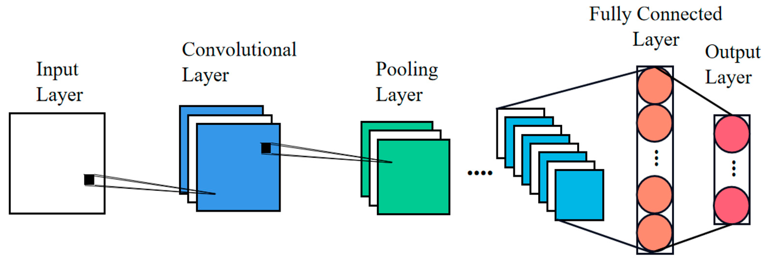
Figure 2.
Structure of the residual block.

Figure 3.
Structure of the CBAM.

Figure 4.
Network structure of the proposed model.
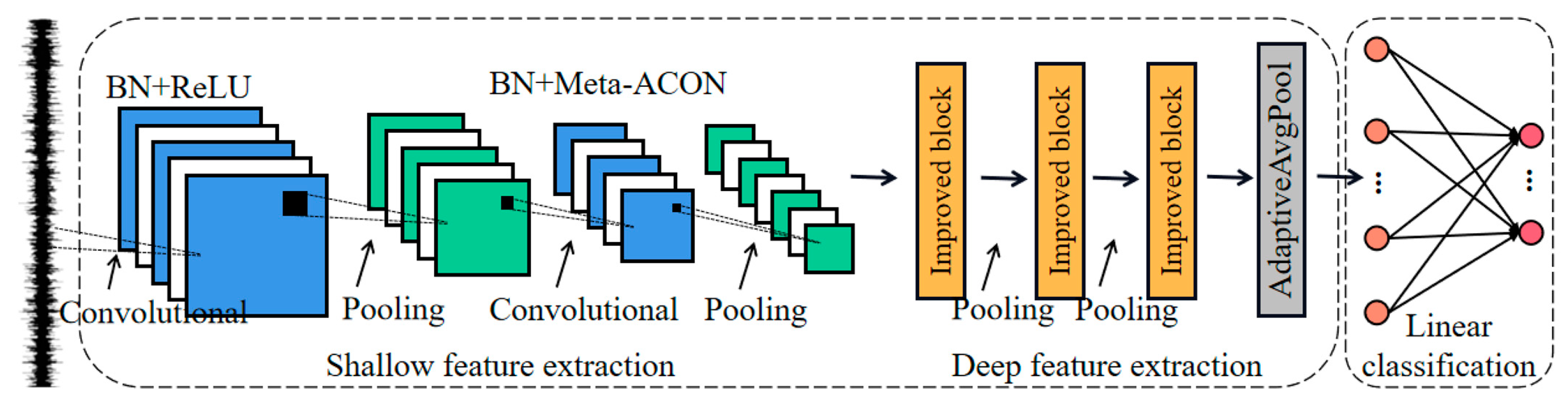
Figure 5.
Structure of improved residual block.
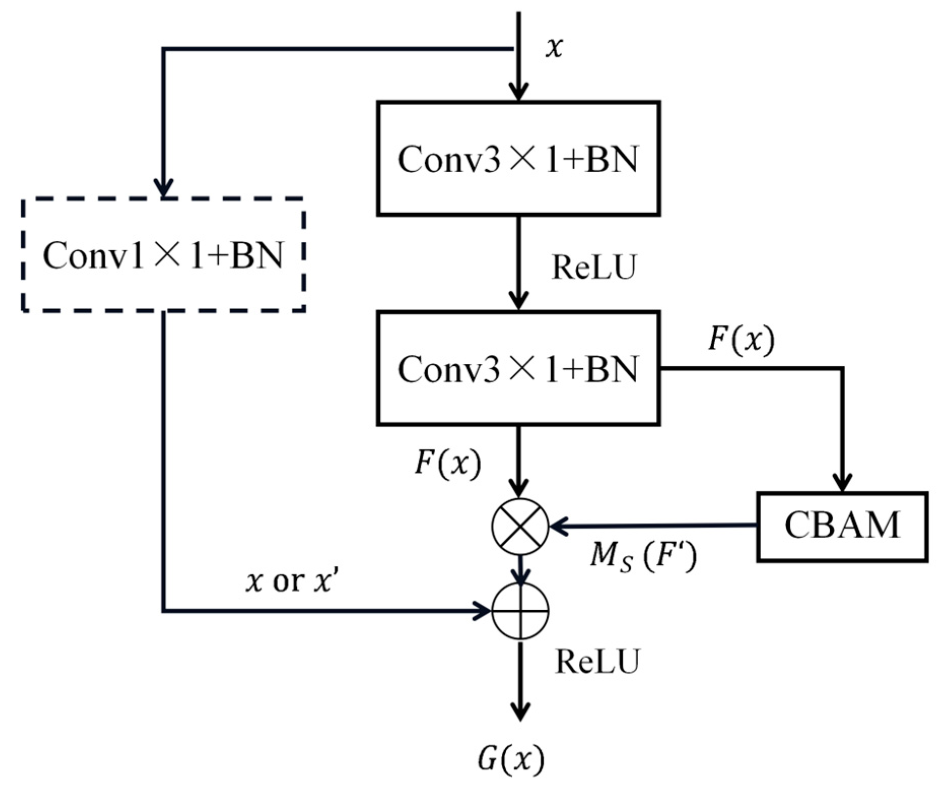
Figure 6.
CWRU bearing faults experimental equipment.

Figure 7.
The process of sampling time domain signals using sliding windows.

Figure 8.
The time domain images, (a–j) corresponds to 0~9 of the fault type label.


Figure 9.
Fault diagnosis flows.

Figure 10.
Experimental results: (a) Accuracy line; (b) Loss line.

Figure 11.
Fault diagnosis results of different models under variable noise.

Figure 12.
The confusion matrix of the fault diagnostic results (4 dB): (a) Confusion matrix of WDCNN; (b) Confusion matrix of the proposed model.
Figure 12.
The confusion matrix of the fault diagnostic results (4 dB): (a) Confusion matrix of WDCNN; (b) Confusion matrix of the proposed model.

Figure 13.
The domain shift phenomenon theory.

Figure 14.
Fault diagnosis results of different models under variable load domain.

Figure 15.
The ablation experiment’s results.

Figure 16.
The visualization of fault diagnosis results (01): (a) MSCNN; (b) WDCNN; (c) Proposed model; (d) Proposed model without using Meta ACON-C; (e) Proposed model without embedding the CBAM; (f) Proposed model without embedding the CBAM and without using Meta ACON-C.
Figure 16.
The visualization of fault diagnosis results (01): (a) MSCNN; (b) WDCNN; (c) Proposed model; (d) Proposed model without using Meta ACON-C; (e) Proposed model without embedding the CBAM; (f) Proposed model without embedding the CBAM and without using Meta ACON-C.


Table 1.
Model Parameters.
| Network Structure | Parameter Setting 2 | Output Size | Activation Function |
|---|---|---|---|
| Conv_1 | k = 64, s = 16, p = 24 | 32 × 64 | ReLU |
| MaxPooling_1 | k = s = 2 | 32 × 32 | - |
| Conv_2 | k = 3, s = 1, p = 1 | 32 × 32 | Meta ACON-C |
| MaxPooling_2 | k = s = 2 | 32 × 16 | - |
| Improved block with CBAM 1 | - | 32 × 16 | ReLU |
| MaxPooling_3 | k = s = 2 | 32 × 8 | - |
| Improved block with CBAM | - | 64 × 8 | ReLU |
| MaxPooling_4 | k = s = 2 | 64 × 4 | - |
| Improved block with CBAM | - | 128 × 4 | ReLU |
| Adaptive AvgPooling | - | 128 × 1 | - |
| Fully connected layer | in = 128, out = 10 | 10 | - |
1 Improved block with CBAM is the same structure as in Section 2.5.2, and the parameters are already listed in the text. 2 In Parameter Setting, “k” is kernel size, “s” is stride, “p” is padding, “in/out” is in/out features.
Table 2.
The one-to-one correspondence between load and speed.
| Motor Load | 0HP | 1HP | 2HP | 3HP |
| Approx. Speed | 1797 r/min | 1772 r/min | 1750 r/min | 1730 r/min |
Table 3.
Experimental data.
| Fault Position | Fault Sizes (Inches) | Load | |||
|---|---|---|---|---|---|
| 0HP | 1HP | 2HP | 3HP | ||
| Normal | / | *+ 1 | *+ | *+ | *- |
| IRF | 0.007 | *+ | *+ | *+ | *- |
| 0.014 | *+ | *+ | *+ | *- | |
| 0.021 | *+ | *+ | *+ | *- | |
| 0.028 | *- | *- | *- | *- | |
| BF | 0.007 | *+ | *+ | *+ | *- |
| 0.014 | *+ | *+ | *+ | *- | |
| 0.021 | *+ | *+ | *+ | *- | |
| 0.028 | *- | *- | *- | *- | |
| ORF | 0.007 | *+ | *+ | *+ | *- |
| 0.014 | *+ | *+ | *+ | *- | |
| 0.021 | *+ | *+ | *+ | *- | |
| 0.028 | - | - | - | - | |
1 Mark “*+” data available and will be used as experimental data, mark “*-” data available but will not be used as experimental data, mark “-” data unavailable.
Table 4.
The division of the experimental sample(0HP).
| Fault Sizes (Inches) | Fault Position | Tra/Val/Test 1 | Fault Type Label |
|---|---|---|---|
| None | Normal | 240/80/80 | 0 |
| 0.007 | IRF | 240/80/80 | 1 |
| RBF | 240/80/80 | 2 | |
| ORF | 240/80/80 | 3 | |
| 0.014 | IRF | 240/80/80 | 4 |
| RBF | 240/80/80 | 5 | |
| ORF | 240/80/80 | 5 | |
| 0.021 | IRF | 240/80/80 | 7 |
| RBF | 240/80/80 | 8 | |
| ORF | 240/80/80 | 9 |
1 Tra/Val/Test represent the number of samples for training, validation and testing, respectively. In the diagnostic process, for the model, the test/val samples is unlabeled.
Table 5.
Diagnostic accuracy in certain load condition data.
| Load Condition of Data | Accuracy (%) |
|---|---|
| 0 HP | 100 |
| 1 HP | 100 |
| 2 HP | 100 |
| 0~2 HP 1 | 100 |
1 0~2HP means that the tra3 × 240, val3 × 80, and test3 × 80 in single Fault Type Label, samples are uniformly from these three different loads.
Table 6.
Comparison of similar approaches.
| Reference | Domain of Input Data | Whether End-to-End | Average Accuracies Results (%) 1 |
|---|---|---|---|
| Wang et al. [41] | Time | Yes | 90.58 |
| Hou et al. [8] | Frequency | No | 91.44 |
| Zhang et al. [15] | Time | Yes | 94.90 |
| Proposed model | Time | Yes | 97.68 |
1 Average accuracy of five replicate experiments is considered as one result, five different noises have five results, and finally the five results are averaged.
Table 7.
Evaluation metrics of the proposed model.
| Fault Type Label | Precision (%) | Recall (%) | F1 Score (%) |
|---|---|---|---|
| 0 | 98.76 | 100 | 99.38 |
| 1 | 100 | 100 | 100 |
| 2 | 100 | 95 | 97.43 |
| 3 | 100 | 100 | 100 |
| 4 | 84.21 | 100 | 91.43 |
| 5 | 91.95 | 100 | 95.81 |
| 6 | 100 | 75 | 85.71 |
| 7 | 100 | 100 | 100 |
| 8 | 98.76 | 100 | 99.38 |
| 9 | 100 | 100 | 100 |
Table 8.
Domain details of the experiments.
| Domain Type | Source Domain | Target Domain | |
|---|---|---|---|
| Description | Labeled signal samples under a single load | Unlabeled signal samples under another load | |
| Domain details | Train samples of 0 HP | Test samples of 1 HP | Test samples of 2 HP |
| Train samples of 2 HP | Test samples of 1 HP | Test samples of 0 HP | |
| Train samples of 1 HP | Test samples of 0 HP | Test samples of 2 HP | |
| Objectives of the experiments | Generalize the fault diagnosis knowledge learned from source domain to target domain, diagnose samples in the target domain | ||
Table 9.
The details of differentiating ablation comparison models.
| Names of the Models | Optimization Techniques 1 | |
|---|---|---|
| Embedding CBAM | Using Meta ACON-C | |
| Base | × | × |
| Base + A | √ | × |
| Base +B | × | √ |
| Base + A + B (proposed model) | √ | √ |
1 Mark “√” means that the optimization techniques is applied. Mark “×” means that the optimization techniques is not applied.
Disclaimer/Publisher’s Note: The statements, opinions and data contained in all publications are solely those of the individual author(s) and contributor(s) and not of MDPI and/or the editor(s). MDPI and/or the editor(s) disclaim responsibility for any injury to people or property resulting from any ideas, methods, instructions or products referred to in the content. |
© 2023 by the authors. Licensee MDPI, Basel, Switzerland. This article is an open access article distributed under the terms and conditions of the Creative Commons Attribution (CC BY) license (https://creativecommons.org/licenses/by/4.0/).
Share and Cite
MDPI and ACS Style
Qin, H.; Pan, J.; Li, J.; Huang, F. Fault Diagnosis Method of Rolling Bearing Based on CBAM_ResNet and ACON Activation Function. Appl. Sci. 2023, 13, 7593. https://doi.org/10.3390/app13137593
AMA Style
Qin H, Pan J, Li J, Huang F. Fault Diagnosis Method of Rolling Bearing Based on CBAM_ResNet and ACON Activation Function. Applied Sciences. 2023; 13(13):7593. https://doi.org/10.3390/app13137593
Chicago/Turabian StyleQin, Haihua, Jiafang Pan, Jian Li, and Faguo Huang. 2023. "Fault Diagnosis Method of Rolling Bearing Based on CBAM_ResNet and ACON Activation Function" Applied Sciences 13, no. 13: 7593. https://doi.org/10.3390/app13137593
Note that from the first issue of 2016, this journal uses article numbers instead of page numbers. See further details here.