Prediction of MAG Welding Formation Based on Fuzzy Interpolation Reasoning

Abstract

Welding is an important production and processing method in industrial production. Due to the uncertainty of its process and the complexity of its mechanism, it is challenging to construct an accurate welding process parameter model to describe it. Fuzzy interpolation reasoning is a valuable tool in the realm of intelligent systems. It helps to reduce the complexity of fuzzy models and can be used for reasoning in fuzzy systems with sparse rule bases. This paper provides an interpolation reasoning method that combines fuzzy set distance and similarity. The proposed method is applied to welding forming predictions, and welding penetration is predicted by the given welding current and speed. The results show that the algorithm has high calculation accuracy.

1. Introduction

Welding technology is an important production and processing method in industrial production. Due to its low cost, high efficiency and reliable connection, it is widely used in the metal connections of marine production. However, welding is a highly nonlinear, time-varying and multicoupling typically complex process; thus, it is difficult to describe accurately by a model. Usually, the quality of welded joints is directly affected by the welding input parameters, as the selection of welding process parameters has a significant impact on the quality of welded joints. At present, the determination of welding process parameters and the prediction of welding formation quality rely more on the experience and subjective judgment of professional and skilled welders. Fuzzy logic can perform well in such situations. In [1,2,3,4], fuzzy logic was used to predict the weld-forming quality and achieved good results. However, the weld-forming prediction model based on traditional fuzzy inference methods has certain limitations. For sparse fuzzy rule bases with incomplete knowledge, traditional fuzzy reasoning methods (like the widely used Mamdani inference method) cannot obtain effective results. It is very meaningful to seek a method for predicting welding formation in a sparse rule base of the welding process.

Uncertain information is inevitable in practical applications. One of the challenges for intelligent systems is how to effectively handle uncertainty to achieve more accurate decision-making. So far, there have been many effective studies on uncertain information, like intuitionistic fuzzy sets [5,6], extension of intuitionistic fuzzy sets [7], complex decision-making [8,9], evidential reasoning [10,11], and fuzzy set theory [12]. Since the theory of fuzzy sets was put forward in 1965, it has gradually become a powerful tool to manage the problems of fuzziness and uncertainty, especially for systems based on fuzzy rules, which have been applied in many fields and work effectively [13,14]. The most widely used fuzzy system is the inference system based on fuzzy rules. Fuzzy inference is an important part of intelligent systems such as fuzzy control, fuzzy expert systems and fuzzy decision support systems. However, traditional fuzzy inference techniques require that any input value must fire at least one fuzzy rule in the rule base, so that the fuzzy inference system can operate normally. However, in the process of industrial production, significant time and energy are required to construct a complete rule base that completely covers the entire input domain. However, due to incomplete knowledge, it is not easy to build a complete rule base. When the rule antecedents in the rule base cannot match the given observations, the traditional fuzzy reasoning method will not derive the inference consequence.

Kóczy and Hirota [15] proposed the fuzzy rule interpolation method (FRI) in 1993 to solve the above problems, which provides a new way for reasoning under sparse rule bases. In recent years, some fuzzy interpolation reasoning methods applicable to sparse rule bases have been proposed. These interpolation reasoning methods can be summarized into two forms: one is fuzzy rule-interpolation reasoning based on nontransformation methods, and the other is interpolation reasoning based on intermediate rule transformation. The KH method is the earliest nontransformation type of fuzzy rule-interpolation reasoning, but in some cases the reasoning result is not convex. Qiao et al. [16] proposed an improved method to ensure the convexity of inference conclusions by using similar transfer inference. Baranyi et al. [17] improved the method of rule interpolation based on α-cut set to avoid abnormal consequences. Wang et al. [18] proposed an interpolation reasoning method based on geometric similarity according to the proportion of the geometric area enclosed by the input facts and rule antecedents. Wang Baowen et al. [19] proposed a fuzzy LaGrange’s interpolation reasoning method based on geometric parameters according to slope. Relying on transforming intermediate rules, such as those given in Huang and Shen [20,21], Jin et al. [22], Yang et al. [23] and Naik et al. [24], have been popularly studied and widely applied, despite their relative recency. Huang and Shen [20], [21] used the gravity feature of membership function graph to construct intermediate rules, then used scale and move transformations to obtain the reasoning consequences. Chen et al. [25] selected a subset of rules from the sparse rule base with an embedded rule-weighting scheme for the automatic assembling of the intermediate rule. Xu et al. [26] measured and subsequently added certain interpolated rules that are deemed of high value into the sparse rule base. In addition, some interpolation methods [25,27] using the weighted rule-interpolation scheme, which generates attribute weights given a sparse rule base and integrates them into nonweighted FRI for classification and prediction. Through continuous development, some methods were successfully applied to control and prediction [28,29,30,31].

Most of the above methods have some shortcomings, and some of the reasoning results of these methods will lead to nonconvex Fuzzy set [15], poor applicability [19], and high computational complexity [20,21]. The distance and similarity of fuzzy sets are important concepts to judge the degree of difference between two fuzzy sets. In the existing research, the fuzzy set distance is mostly defined based on the cut set and representative value of the fuzzy set, which simplifies the calculation of the fuzzy set distance, but may lead to an insufficient description of the distance reflecting the whole fuzzy set. Therefore, this paper defines the distance of fuzzy sets by normalizing the Euclidean distance. The intermediate rules are constructed by calculating the distance between the observed values and the fuzzy sets of adjacent rules. The final inference conclusion is determined according to the similarity of fuzzy sets. This method can obtain inference conclusions that satisfy the normality and convexity of fuzzy sets, and are also applicable to different types of Fuzzy sets. It is of great significance to improve the interpolation inference method system.

Welding is an important process in industrial production. Due to the complexity of its process mechanism, it is difficult to describe through precise mathematical models. At present, the prediction, decision-making, and control of welding processes are usually completed by the experience and knowledge of experts and technicians. For this type of knowledge, it is more appropriate to use fuzzy language to describe it. The establishment of welding process parameter models usually requires a large number of prior experiments to complete. For the widely used fuzzy inference model—Mamdani fuzzy inference model—the inference process requires a complete rules base. It is difficult to construct a welding formation prediction model using such inference models. The more rules reflect the relationship between welding process parameters and welding formation quality, the more parameter experiments are required to establish the rules. The fuzzy interpolation inference method does not require a complete rules base to achieve inference. To address the above issues, we propose a welding formation prediction method based on fuzzy interpolation inference, and provide an idea for achieving efficient and convenient welding formation prediction. More importantly, fuzzy interpolation reasoning has better application prospects for achieving welding process parameter designs and real-time control of welding formation.

The paper is organized as follows. For completeness, Section 2 reviews the KH methods and HS methods. Section 3 describes the new interpolative reasoning method. Section 4 provides an application example of MAG welding formation prediction. Finally, in Section 5, we discuss our conclusions.

2. Overview of Fuzzy Interpolation

Fuzzy rule interpolation is an inference technique for fuzzy rule bases where the antecedents do not cover the whole input universe. It addresses the key limitations of Compositional Rule of Inference (CRI) that requires a dense fuzzy rule base which fully covers the entire problem domain. The KH method was proposed by Kóczy and Hirota in 1993, which is also the earliest fuzzy interpolation inference method based on α-cut of the fuzzy set, providing a theoretical basis for many subsequent methods. In this section, the original KH interpolation reasoning method and popular HS methods are introduced.

Suppose that $A_1\Rightarrow B_1$ and $A_2\Rightarrow B_2$ are two adjacent fuzzy rules on universe X and Y. Assume that the observation value is $A^{\ast }=(a_1^{\ast },a_2^{\ast },a_3^{\ast })$, and $A_1\prec A^{\ast }\prec A_2$.

Rule 1: If x₁ is A₁, then y is B₁

Rule 2: If x₁ is A₂, then y is B₂

Observation: If x is A*

where $A_i=(a_{i1},a_{i2},a_{i3})$, $i=1,2$, where $a_{i1}$ and $a_{i3}$ are the left and right support vertexes, respectively, and $a_{i2}$ is the normal point of the fuzzy set, as shown in Figure 1.

2.1. KH Method [15]

The KH method is the earliest proposed interpolation inference method, which provides a basic idea for many types of interpolation inference methods. The KH linear interpolation is mainly based on $\alpha -$ cut of the fuzzy set, and the basic idea of the KH method can be written as

$$\frac{d(A^{\ast },A_1)}{d(A^{\ast },A_2)}=\frac{d(B^{\ast },B_1)}{d(B^{\ast },B_2)}$$

(1)

According to the resolution principle of fuzzy sets, the lower and upper distance $d_L(\cdot ,\cdot )$ and $d_U(\cdot ,\cdot )$ are defined as

$$\frac{d_L(A_{\alpha }^{\ast },A_{1\alpha })}{d_L(A_{\alpha }^{\ast },A_{2\alpha })}=\frac{d_L(B_{\alpha }^{\ast },B_{1\alpha })}{d_L(B_{\alpha }^{\ast },B_{2\alpha })}$$

(2)

$$\frac{d_U(A_{\alpha }^{\ast },A_{1\alpha })}{d_U(A_{\alpha }^{\ast },A_{2\alpha })}=\frac{d_U(B_{\alpha }^{\ast },B_{1\alpha })}{d_U(B_{\alpha }^{\ast },B_{2\alpha })}$$

(3)

where $\alpha$ means that the $\alpha$-cut of the fuzzy set.

Then the lower and upper values of the result can be written as

$$inf\left\{B_{\alpha }^{\ast }\right\}=\frac{d_L(A_{\alpha }^{\ast },A_{1\alpha })\times inf\left\{B_{2\alpha }\right\}+d_L(A_{\alpha }^{\ast },A_{2\alpha })\times inf\left\{B_{1\alpha }\right\}}{d_L(A_{\alpha }^{\ast },A_{1\alpha })+d_L(A_{\alpha }^{\ast },A_{2\alpha })}$$

(4)

$$sup\left\{B_{\alpha }^{\ast }\right\}=\frac{d_U(A_{\alpha }^{\ast },A_{1\alpha })\times sup\left\{B_{2\alpha }\right\}+d_U(A_{\alpha }^{\ast },A_{2\alpha })\times sup\left\{B_{1\alpha }\right\}}{d_U(A_{\alpha }^{\ast },A_{1\alpha })+d_U(A_{\alpha }^{\ast },A_{2\alpha })}$$

(5)

where $inf\left\{B_{\alpha }^{\ast }\right\}$ and $sup\left\{B_{\alpha }^{\ast }\right\}$ represent the infimum and supremum of $B_{\alpha }^{\ast }$, respectively.

Let

$${\lambda }_L=\frac{d_L(A_{\alpha }^{\ast },A_{1\alpha })}{d_L(A_{2\alpha },A_{1\alpha })}$$

(6)

$${\lambda }_U=\frac{d_U(A_{\alpha }^{\ast },A_{1\alpha })}{d_U(A_{2\alpha },A_{1\alpha })}$$

(7)

Then, (4) and (5) can be rewritten as:

$$inf\left\{B_{\alpha }^{\ast }\right\}=(1-{\lambda }_L)inf\left\{B_{1\alpha }\right\}+{\lambda }_{L}inf\left\{B_{2\alpha }\right\}$$

(8)

$$sup\left\{B_{\alpha }^{\ast }\right\}=(1-{\lambda }_U)sup\left\{B_{1\alpha }\right\}+{\lambda }_{U}sup\left\{B_{2\alpha }\right\}$$

(9)

Finally, $B^{\ast }=(inf\{B_{\alpha }^{\ast }\},sup\{B_{\alpha }^{\ast }\})$, and the consequence B* can be constructed

$$B^{\ast }={\displaystyle \underset{\alpha \in [0,1]}{{\displaystyle \cup }}\alpha }{B}_{\alpha }^{\ast }$$

(10)

However, this linear interpolation cannot guarantee the convexity of the derived fuzzy sets even if the fuzzy sets involved in the given rules and observations are convex and normal.

2.2. HS Method [20]

The HS method is a representative method based on intermediate rule-interpolation inference. The main process of the HS method is as follows: let A be a triangular fuzzy set, and $A=(a_1,a_2,a_3)$. Then the representative value Rep(A) of A can be defined by

$$Rep(A)=\frac{a_1+a_2+a_3}{3}$$

(11)

The first step of the HS method is to construct a new fuzzy set $A^{\prime }$ by the distance ratio of representative value ${\lambda }_{Rep}$, which has the same representative value of A*. Let

$$\begin{array}{ll}{\lambda }_{Rep}& =\frac{d(A_1,A^{\ast })}{d(A_1,A_2)}\\ & =\frac{d(Rep(A_1),Rep(A^{\ast }))}{d(Rep(A_1),Rep(A_2))}\end{array}$$

(12)

Then, the fuzzy set $A^{\prime }(a_1^{\prime },a_2^{\prime },a_3^{\prime })$ can be obtained, and the parameters of $A^{\prime }$ are determined as follows:

$$a_1^{\prime }=(1-{\lambda }_{Rep})a_{11}+{\lambda }_{Rep}{a}_{21}$$

(13)

$$a_2^{\prime }=(1-{\lambda }_{Rep})a_{12}+{\lambda }_{Rep}{a}_{22}$$

(14)

$$a_3^{\prime }=(1-{\lambda }_{Rep})a_{13}+{\lambda }_{Rep}{a}_{23}$$

(15)

The fuzzy set $B^{\prime }(b_1^{\prime },b_2^{\prime },b_3^{\prime })$ can be obtained the same way, and the parameters of $B^{\prime }$ are determined as follows:

$$B^{\prime }=(1-{\lambda }_{Rep})B_1+{\lambda }_{Rep}{B}_2$$

(16)

The HS method uses the following two transformations:

(1) Scale transformation: Scale operation from $A^{\prime }$ to ${\widehat{A}}^{\prime }$ by the scale rate s, where the scale rate s is calculated as follows:

$$s=\frac{a_3-a_1}{a_3^{\prime }-a_1^{\prime }}$$

(17)

Each characteristic value of ${\widehat{A}}^{\prime }$ can be calculated as follows:

$${\widehat{a}}_1^{\prime }=\frac{(1+2s)a_1^{\prime }+(1-s)a_2^{\prime }+(1-s)a_3^{\prime }}{3}$$

(18)

$${\widehat{a}}_2^{\prime }=\frac{(1-s)a_1^{\prime }+(1+2s)a_2^{\prime }+(1-s)a_3^{\prime }}{3}$$

(19)

$${\widehat{a}}_3^{\prime }=\frac{(1-s)a_1^{\prime }+(1-s)a_2^{\prime }+(1+2s)a_3^{\prime }}{3}$$

(20)

$B^{\prime }$ can be converted to $\widehat{B^{\prime }}$ the same way.

(2) Move transformation: The move operation shifts the position of ${\widehat{A}}^{\prime }$ to become the same as that of $A^{\ast }$, and the move ratio m can be calculated as follows:

$$m=\left\{\begin{array}{ll}\frac{3\left(a_1-{\widehat{a}}_1^{\prime }\right)}{{\widehat{a}}_2^{\prime }-{\widehat{a}}_1^{\prime }},\hfill & if a_1\ge {\widehat{a}}_1^{\prime }\hfill \\ \frac{3\left(a_1-{\widehat{a}}_1^{\prime }\right)}{{\widehat{a}}_3^{\prime }-{\widehat{a}}_2^{\prime }},\hfill & if a_1\le {\widehat{a}}_1^{\prime }\hfill \end{array}\right.$$

(21)

Then, move transformation is applied to construct consequence $B^{\ast }=(b_1^{\ast },b_2^{\ast },b_3^{\ast })$:

$$\left\{\begin{array}{c}{b}_1^{\ast }={\widehat{b}}_1^{\prime }+m\cdot \gamma \\ b_2^{\ast }={\widehat{b}}_2^{\prime }-2m\cdot \gamma \\ b_3^{\ast }={\widehat{b}}_3^{\prime }+m\cdot \gamma \end{array}\right.\begin{array}{cc}\gamma =\left\{\begin{array}{c}\frac{{\widehat{b}}_2^{\prime }-{\widehat{b}}_1^{\prime }}{3}\\ \frac{{\widehat{b}}_3^{\prime }-{\widehat{b}}_2^{\prime }}{3}\end{array}\right.& \begin{array}{c}if m\ge 0\\ otherwise\end{array}\end{array}$$

(22)

Finally, the HS method obtains the fuzzy interpolative reasoning consequence B* by transforming $B^{\prime }$ with the same scale rate s and the same moving ratio m between the fuzzy sets $A^{\ast }$ and $A^{\prime }$. For more details, refer to [20].

3. The Fuzzy Interpolation Methods

Fuzzy rule interpolation is an inference technique for fuzzy rule bases where the antecedents do not cover the whole input universe. The distance and similarity of fuzzy sets are important concepts to judge the degree of difference between two fuzzy sets. In this section, a new fuzzy interpolation inference method is introduced. In this paper, the specification that the distance of $D(A,B)$ is defined by the normalized Euclidean distance.

3.1. Single Antecedent with Triangular Fuzzy Sets

Suppose that $A_1\Rightarrow B_1$ and $A_2\Rightarrow B_2$ are two adjacent fuzzy rules on universe X and Y. Assume that the observation value is $A^{\ast }=(a_1^{\ast },a_2^{\ast },a_3^{\ast })$, and $A_1<A^{\ast }<A_2$.

Rule 1: If x₁ is A₁, then y is B₁

Rule 2: If x₁ is A₂, then y is B₂

Observation: If X is A^*

where $A_i=(a_{i1},a_{i2},a_{i3})$, $B_i=(b_{i1},b_{i2},b_{i3})$, $i=1,2$.

The proposed fuzzy interpolation reasoning method is presented as follows.

(Step 1) Construct a new intermediate fuzzy set $A^{\prime }$ by the distance factor ${\lambda }_D$ and $0\le {\lambda }_D\le 1$. The distance $D(A_1,A^{\ast })$ and $D(A_1,A_2)$ between $A_1$ and $A^{\ast }$, $A_1$ and $A_2$ can be calculated as follows:

$$D(A_1,A^{\ast })={\left[\frac{1}{3}{\displaystyle \sum _{i=1}^3{(a_i^{\ast }-a_{1i})}^2}\right]}^{1/2}$$

(23)

$$D(A_1,A_2)={\left[\frac{1}{3}{\displaystyle \sum _{i=1}^3{(a_{2i}-a_{1i})}^2}\right]}^{1/2}$$

(24)

then, the distance factor ${\lambda }_D$ can be calculated as follows:

$${\lambda }_D=\frac{D(A_1,A^{\ast })}{D(A_1,A_2)}$$

(25)

Based on the value of ${\lambda }_D$, each characteristic value of $A^{\prime }$ can be calculated as follows:

$$a_1^{\prime }=(1-{\lambda }_D)a_{11}+{\lambda }_D{a}_{21}$$

(26)

$$a_2^{\prime }=(1-{\lambda }_D)a_{12}+{\lambda }_D{a}_{22}$$

(27)

$$a_3^{\prime }=(1-{\lambda }_D)a_{13}+{\lambda }_D{a}_{23}$$

(28)

The intermediate fuzzy set $A^{\prime }$ and observation $A^{\ast }$ have the same distance from $A_1$.

$$\begin{array}{r}\hfill D(A_1,A^{\ast })=D(A_1,A^{\prime })\end{array}$$

(29)

The consequent part $B^{\prime }$ corresponding to the antecedent of the intermediate rule $A^{\prime }$ can be constructed in the same way:

$$B^{\prime }=(1-{\lambda }_D)B_1+{\lambda }_D{B}_2$$

(30)

(Step 2) Find the width similarity of observed value $A^{\ast }$ and the intermediate $A^{\prime }$.

Suppose there is a certain degree of similarity between the antecedent of observed value $A^{\ast }$ and the intermediate $A^{\prime }$, in which case it can be intuitively believed that the same degree of similarity exists between the consequent part $B^{\ast }$ and $B^{\prime }$. Therefore, the membership function can be divided into left and right parts. According to the observation value $A^{\ast }$ and intermediate fuzzy set $A^{\prime }$ shown in Figure 2, the left and right similarity ratio $S^L(A^{\ast },A^{\prime })$ and $S^R(A^{\ast },A^{\prime })$ of antecedent $A^{\ast }$ and $A^{\prime }$ can be calculated by the following formula:

$$S^L(A^{\ast },A^{\prime })=\frac{a_2^{\ast }-a_1^{\ast }}{a_2^{\prime }-a_1^{\prime }}$$

(31)

$$S^R(A^{\ast },A^{\prime })=\frac{a_3^{\ast }-a_2^{\ast }}{a_3^{\prime }-a_2^{\prime }}$$

(32)

(Step 3) Find the parameter values of $B^{\ast }$ by the distance and width similarity.

According to step 1, it can be seen that the intermediate fuzzy set $A^{\ast }$ and observation $A^{\prime }$ have the same distance from $A_1$. Then, in the same way, it can be judged that $B^{\ast }$ and $B^{\prime }$ have the same distance from $B_1$, and according to the width similarity, the following equation can be obtained:

$$\left\{\begin{array}{c}D(B^{\ast },B_1)=D(B^{\prime },B_1)\\ S^L(A^{\ast },A^{\prime })=S^L(B^{\ast },B^{\prime })\\ S^R(A^{\ast },A^{\prime })=S^R(B^{\ast },B^{\prime })\end{array}\right.$$

(33)

By substituting (30) and (31) into Equation (32), the following formula can be obtained:

$$\left\{\begin{array}{c}{(b_1^{\ast }-b_{11})}^2+{(b_2^{\ast }-b_{12})}^2+{(b_3^{\ast }-b_{13})}^2=\\ {(b_1^{\prime }-b_{11})}^2+{(b_2^{\prime }-b_{12})}^2+{(b_3^{\prime }-b_{13})}^2\\ b_2^{\ast }=b_1^{\ast }+S^L(A^{\ast },A^{\prime })\cdot (b_2^{\prime }-b_1^{\prime })\\ b_3^{\ast }=b_2^{\ast }+S^R(A^{\ast },A^{\prime })\cdot (b_3^{\prime }-b_2^{\prime })\end{array}\right.$$

(34)

According to Equation (33), the reasoning consequence $B_1^{\ast }$ and $B_2^{\ast }$ can be obtained. The final inference consequence is determined by the principle of maximum similarity of fuzzy sets.

The similarity SS(A, B) between fuzzy sets A and B can be calculated according to the following formula:

$$SS(A,B)={(1+D(A,B))}^{-1}$$

(35)

By following the above steps, we can draw the inference consequence B* about the observed values A*.

3.2. Multiple Antecedent Variables with Complex Polygonal Fuzzy Sets

Because the trapezoidal membership function is the most typical of polygonal membership functions, this section will take the membership function of the trapezoidal fuzzy set as an example to extend the above interpolation reasoning method. Because the reasoning process of a single antecedent variable is similar to that of multiple antecedents, this section will take the multiple antecedents of the trapezoidal fuzzy set membership function reasoning model as an example.

Assume that the trapezoidal membership function reasoning model is as follows:

Rule i: If x₁ is A_1i and … and x_mi is A_mi, then y is B_i

Rule j: If x₁ is A_1j and … and x_mj is A_mj, then y is B_j

Observation: If X is A*

where $A_{ki}=(a_1^{ki},a_2^{ki},a_3^{ki},a_4^{ki})$ and k = 1, 2,…, m.

(Step 1) Construct a new intermediate fuzzy set $A_k^{\prime }$ by the distance factor ${\lambda }_{Dk}$ and $0\le {\lambda }_{Dk}\le 1$.

$$\begin{array}{r}\hfill {\lambda }_{Dk}=\frac{D_k(A_{ki},A_k^{\ast })}{D_k(A_{ki},A_{kj})}=\frac{{\left[\frac{1}{4}{\displaystyle \sum _{n=1}^4{(a_n^{k^{\ast }}-a_n^{ki})}^2}\right]}^{1/2}}{{\left[\frac{1}{4}{\displaystyle \sum _{n=1}^4{(a_n^{k_j}-a_n^{k_i})}^2}\right]}^{1/2}}\end{array}$$

(36)

Based on the value of ${\lambda }_{Dk}$, each characteristic value of $A_k^{\prime }$ can be calculated as follows:

$$A_k^{\prime }=(1-{\lambda }_{Dk})A_{ki}+{\lambda }_{Dk}{A}_{kj}$$

(37)

The consequent part $B^{\prime }$ corresponding to the antecedent of the intermediate rule $A_k^{\prime }$ can be constructed in the same way, and ${\lambda }_D$ is the arithmetic averages of ${\lambda }_{Dk}$:

$$B^{\prime }=(1-{\lambda }_D)B_i+{\lambda }_D{B}_j$$

(38)

$${\lambda }_D=\frac{1}{m}{\displaystyle \sum }_{k=1}^m{\lambda }_{Dk}$$

(39)

(Step 2) Find the width similarity of observed value $A_k^{\ast }$ and the intermediate $A_k^{\prime }$.

Suppose there is a certain degree of similarity between the antecedent of observed value $A_k^{\ast }$ and the intermediate $A_k^{\prime }$, in that case it can be intuitively believed that the same degree of similarity exists between the consequent part $B^{\ast }$ and $B^{\prime }$. Therefore, the membership function can be divided into left, central and right parts. The left, central and right parts similarity ratio $S_k^L(A_k^{\ast },A_k^{\prime })$, $S_k^C(A_k^{\ast },A_k^{\prime })$, and $S_k^R(A_k^{\ast },A_k^{\prime })$ of antecedent $A_k^{\ast }$ and $A_k^{\prime }$ can be calculated by the following formula:

$$\begin{array}{r}\hfill S_k^L(A_k^{\ast },A_k^{\prime })=\frac{a_2^{k^{\ast }}-a_1^{k^{\ast }}}{a_2^{k^{\prime }}-a_1^{k^{\prime }}}\end{array}$$

(40)

$$\begin{array}{r}\hfill S_k^C(A_k^{\ast },A_k^{\prime })=\frac{a_3^{k^{\ast }}-a_2^{k^{\ast }}}{a_3^{k^{\prime }}-a_2^{k^{\prime }}}\end{array}$$

(41)

$$\begin{array}{r}\hfill S_k^R(A_k^{\ast },A_k^{\prime })=\frac{a_4^{k^{\ast }}-a_3^{k^{\ast }}}{a_4^{k^{\prime }}-a_3^{k^{\prime }}}\end{array}$$

(42)

(Step 3) Find the parameter values of $B^{\ast }$ by the distance and width similarity.

According to step 1, it can be known that the intermediate fuzzy set $A_k^{\prime }$ and observation $A_k^{\ast }$ have the same distance from $A_{k1}$. Then, in the same way, it can judge that $B^{\ast }$ and $B^{\prime }$ have the same distance from $B_1$, and according to the width similarity, the following equation can be obtained:

$$\left\{\begin{array}{c}D(B^{\ast },B_1)=D(B^{\prime },B_1)\\ S^L(A^{\ast },A^{\prime })=S^L(B^{\ast },B^{\prime })\\ S^C(A^{\ast },A^{\prime })=S^C(B^{\ast },B^{\prime })\\ S^R(A^{\ast },A^{\prime })=S^R(B^{\ast },B^{\prime })\end{array}\right.$$

(43)

where $S^L(A^{\ast },A^{\prime })$, $S^c(A^{\ast },A^{\prime })$ and $S^R(A^{\ast },A^{\prime })$ are the average of $S_k^L(A_k^{\ast },A_k^{\prime })$, $S_k^C(A_k^{\ast },A_k^{\prime })$ and $S_k^R(A_k^{\ast },A_k^{\prime })$, respectively.

$$S^L(A^{\ast },A^{\prime })=\frac{1}{k}\sum _{i=1}^k{S}_i^L(A_i^{\ast },A_i^{\prime })$$

(44)

$$S^C(A^{\ast },A^{\prime })=\frac{1}{k}\sum _{i=1}^k{S}_i^C(A_i^{\ast },A_i^{\prime })$$

(45)

$$S^R(A^{\ast },A^{\prime })=\frac{1}{k}\sum _{i=1}^k{S}_i^R(A_i^{\ast },A_i^{\prime })$$

(46)

According to Equation (42), the reasoning consequence $B_1^{\ast }$ and $B_2^{\ast }$ can be obtained. The final inference consequence is determined by the principle of maximum similarity of fuzzy sets according to (34).

By following the above steps, we can draw the inference consequence $B^{\ast }=(b_1,b_2,b_3,b_4)$ about the observed values $A_k^{\ast }$.

3.3. Experimental Result

In this part, several examples are given for the proposed interpolation method and compared with KH methods and HS methods. The examples involve interpolation between two adjacent rules.

Example 1: This example demonstrates the use of the proposed method involving a single antecedent with triangular fuzzy sets. All the conditions and the fuzzy interpolative reasoning consequences for the different methods are shown in

Table 1. Reasoning consequences of Example 1.

Attribute Values	Method	Results
A1 (0,5,6)	KH Method	(6.36,5.38,7.38)
A2 (11,13,14)	HS Method	(5.83,6.26,7.38)
B1 (0,2,4)	Proposed Method	(5.84,6.27,8.27)
B2 (10,11,13)

and Figure 3.

First, according to (24) to (30), $A^{\prime }$ and $B^{\prime }$ can be calculated as $A^{\prime }$ (5.7, 9.15, 10.15) and $B^{\prime }$ (5.19, 6.67, 8.67), respectively. Then, according to the width similarity relationship between the observed $A^{\ast }$ and antecedent of the intermediate rule $A^{\prime }$, the solutions $B_1^{\ast }$ and $B_2^{\ast }$ of Equation (33) can be obtained as $B_1^{\ast }$ (5.84, 6.27, 8.27) and $B_2^{\ast }$ (−3.744, −3.314, −1.314), respectively. The similarity of SS($B_1^{\ast }$,$B^{\prime }$) and SS($B_2^{\ast }$,$B^{\prime }$) can be calculated as SS($B_1^{\ast }$,$B^{\prime }$) = 0.6675 and SS($B_2^{\ast }$,$B^{\prime }$) = 0.0939, according to (35), respectively. Finally, $B_1^{\ast }$ is selected as the final inference consequence as the consequence B* (5.84,6.27,8.27). From Table 1 and Figure 3, it can be seen that the KH method resulted in a nonconvex consequent fuzzy set, and the reasoning consequence of this method and HS method are both reasonable.

Example 2: This example demonstrates the use of the proposed method involving multiple antecedent variables with trapezoidal fuzzy sets. All the conditions and the fuzzy interpolative reasoning consequences for the different methods are shown in

Table 2. Reasoning consequences of Example 2.

Attribute Values	Method	Results
A11 (0,4,5,6), A12 (11,12,13,14)	KH Method	(5.45,5.94,7.13,8.31)
A21 (1,2,3,4), A22 (12,14,15,16)	HS Method	(4.37,5.55,7.48,9.33)
B1 (0,2,3,4)	Proposed Method	(4.79,6.03,8.03,10.03)
B2 (10,11,12,13)

and Figure 3.

First, according to (37) to (38), $A_1^{\prime }$, $A_2^{\prime }$ and $B^{\prime }$ can be calculated as $A_1^{\prime }$ (5.77, 8.19, 9.19, 10.19), $A_2^{\prime }$ (7.17, 8.73, 9.73, 10.73) and $B^{\prime }$ (5.43, 6.88, 7.88, 8.88), respectively. Then, according to the width similarity relationship between the observation and antecedent of the intermediate rule, the solutions $B_1^{\ast }$ and $B_2^{\ast }$ of Equation (43) can be obtained as $B_1^{\ast }$ (4.79, 6.03, 8.03, 10.03) and $B_2^{\ast }$ (−5.14 9, −3.915, −1.915, −0.085), respectively. The similarity SS($B_1^{\ast }$,$B^{\prime }$) and SS($B_2^{\ast }$,$B^{\prime }$) can be calculated as SS($B_1^{\ast }$,$B^{\prime }$) = 0.5604 and SS($B_2^{\ast }$,$B^{\prime }$) = 0.0907, according to (35), respectively. Finally, $B_1^{\ast }$ is selected as the final inference consequence, then B* (4.79, 6.03, 8.03, 10.03). From Table 2 and Figure 4, we can see that three comparative methods can obtain reasonable conclusions, and the conclusion obtained by this method is closer to that of B₂.

4. Welding Formation Prediction

Welding technology is an important production and processing method in industrial production. However, welding is a highly nonlinear, time-varying and multicoupling typical complex process. It is difficult to describe the process with an accurate model. Establishing welding process parameter models usually requires a large number of prior experiments. Therefore, it is difficult to construct a complete fuzzy rule base for the welding process. For a complete rule base, traditional fuzzy reasoning methods can perform well, but in sparse rule bases, such methods seem powerless. Fuzzy interpolation inference can be performed in a sparse rule base. Using a sparse rule library to construct a welding forming prediction model can achieve inference through a sufficient number of fuzzy rules, which can to some extent reduce the difficulty of constructing the model. Therefore, in this section, we propose a welding formation prediction method based on a sparse rule base.

We consider an application of the proposed algorithm for weld forming prediction. Forming quality of the weld is one of the factors affecting the performance of welded joints. There are many factors affecting the forming of the weld. Under the condition that other process conditions remain unchanged, welding current, welding voltage and welding speed are the key factors affecting the forming quality of the weld. Therefore, selecting reasonable welding process parameters is very important to improve the welding quality and production efficiency.

4.1. Welding Process Parameter Model

Metal active gas arc welding (MAG) is a common metal material connection process in industrial production. It is widely used in industrial fields such as machinery, shipbuilding, and chemical engineering due to its high production efficiency and strong welding process stability. The quality of a welding joint is determined by its mechanical properties, which are dependent both on its metallurgical properties and bead geometry, in which weld penetration is one of the important geometric parameters. For arc welding, the penetration of the welded joint depends on many input process parameters, such as welding current, welding speed, voltage, wire feeding speed, gas flow, nozzle plate distance, torch angle, and so on [32,33]. Therefore, the selection of the appropriate welding parameters is crucial for the welding process.

The depth of a weld seam is an important index of welding quality. Two main technological parameters affect the weld depth Y: the welding current X₁ and welding speed X₂ [34]. 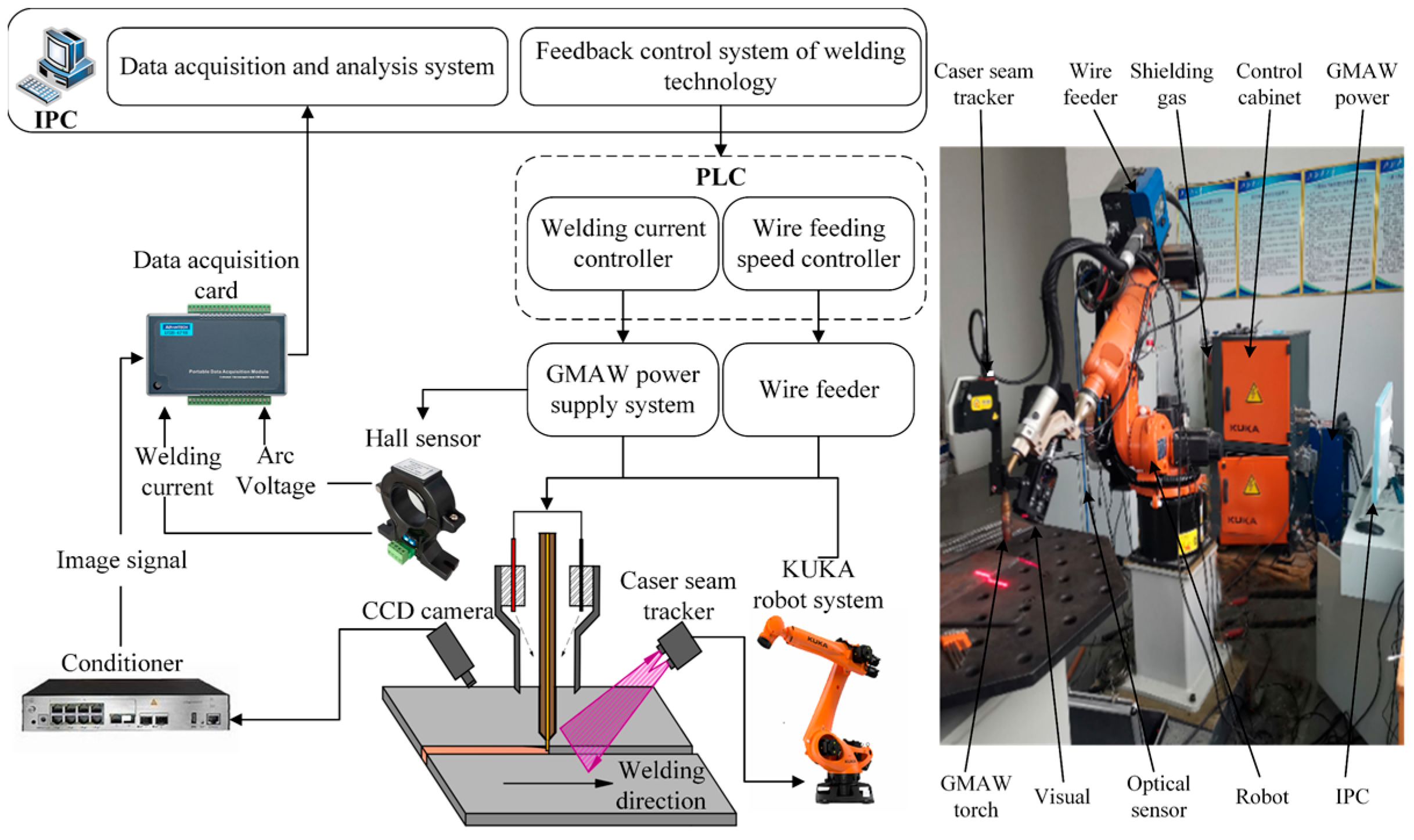In order to establish the relationship between welding depth Y and welding current X₁ and welding speed X₂, an experiment is used that employs the 85%Ar + 15%CO₂ mixed gas arc welding process that is widely used in metal connections [34]. The experimental equipment and conditions are shown in

Table 3. Experimental conditions of MAG welding.

Type	Value
Material for test	Q235 low carbon steel
Welding power	AOTAI Pulse-500RP
Welding position	Flat welding
Shielded gas	85%Ar + 15%CO2
Groove gap (mm)	2
Gas flow (L/min)	15
Welding wire diameter (mm)	1.2
Wire elongation (mm)	15
Welding wire material	H08Mn2SiA
Measuring tools	JGX-2 Tool microscope

and Figure 5, respectively.

Flat and fillet welds are commonly involved in the actual welding process, and in this paper, the experiment adopts commonly used butt-welding connection methods. The welded material is fixed on the welding workbench and the gap between the plates is adjusted to 2 mm before performing the welding operation, as shown in Figure 6.

Then, the welding experiment is performed according to the present welding parameters. Subsequently, the weld penetration measurement is carried out by selecting qualified specimens through welding the appearance and forming the specimens. Due to the inability to measure weld penetration directly, it is necessary to cut the welded specimen. After cutting the welded specimen, the weld penetration can be measured by a JGX-2 Tool microscope. The welding formation and welding penetration are shown in Figure 7. The experimental sample data can be obtained through measurement, as shown in

Table 4. Experimental sample data.

Sample	Current x1 (A)	Speed x2 (mm·min−1)	Depth of Weld y (mm)
1	100	390	3.01
2	100	500	2.62
3	110	375	3.3
4	110	485	2.87
5	120	360	3.6
6	120	470	3.23
7	170	500	4.31
8	170	390	4.77
9	180	375	5.01
10	180	485	4.68
11	190	360	5.23
12	190	470	5.07

.

Based on experimental sample data, the input domain of the welding current X₁ is set to [100, 120] and [170, 190], and the welding speed X₂ is set to [360, 390] and [470, 500]. Using fuzzy language to describe the input domain, fuzzy language variables are defined as small (S) and large (L), which are described by symmetric congruent triangular fuzzy sets, and the membership of welding current X₁ is shown in Figure 8a. The output domain of depth Y is set to [2.62, 3.6] and [4.31, 5.3], and fuzzy language variables defined as Small (S), Medium-small (MS), Medium-large (ML) and Large (L), which are described by symmetric congruent triangular fuzzy sets, and the membership of welding depth Y are shown in Figure 8b.

By defining the fuzzy language of input variables, four fuzzy rules between welding penetration, welding current and welding speed are summarized, as shown in

Table 5. Welding procedure rule.

Welding Current (A)	Welding Speed (mm·min−1)
	S (360–390)	L (470–500)
S (100–120)	MS	S
L (170–190)	L	ML

. Finally, a sparse rule base for the welding forming prediction model can be obtained.

The fuzzy language If–Then description of the sparse rule bases for welding forming prediction is as follows:

Rule 1: If Welding current X1 is S and Welding speed X2 is S, then Welding penetration Y is MS.

Rule 2: If Welding current X1 is S and Welding speed X2 is L, then Welding penetration Y is S.

Rule 3: If Welding current X1 is L and Welding speed X2 is S, then Welding penetration Y is L.

Rule 4: If Welding current X1 is L and Welding speed X2 is L, then Welding penetration Y is ML.

By following the above steps, a sparse rule base of the welding process with only four fuzzy rules can be obtained. Using sparse rule bases to construct inference models not only reduces the difficulty of acquiring modeling knowledge to a certain extent, but also reduces the complexity of fuzzy rule bases without losing generality. For welding, the process of obtaining specific data between welding parameters and welding geometric dimensions is cumbersome and not easy, while using a sparse rule library to describe this relationship is much easier.

4.2. Weld Formation Prediction

In this section, a welding formation prediction process based on a sparse rule base was designed using the method proposed in this article. The main steps of welding formation prediction based on fuzzy interpolation reasoning are as follows:

Step1 Fuzzification: The same triangular fuzzy set as the input variable antecedent is used for fuzzification. The real value of the input variable can be fuzzified by the same triangular membership function with base width b and height 1. Suppose that the input variable of the welding current is $x_1^{\ast }$; it can be fuzzified by the same triangular membership function whose base width is b and membership value at $x_1^{\ast }$ is 1.

Step2 Inference: First, calculate the distance between the input value and the antecedent of adjacent rule by (26) to (30), then construct intermediate rules. Then according to (33), $B_1^{\ast }$ and $B_2^{\ast }$ can be obtained. Finally, the inference consequence B* can be drawn according to the maximum similarity by (35).

Step3 Defuzzification: The result derived from the inference is a family of fuzzy sets, so it is necessary to determine a real value of the weld depth that corresponds to these fuzzy values. Here, the maximum membership principle is adopted for defuzzification. Let y* be a real value of the output B*, and y* can be obtained by

$$B^{\ast }(y^{\ast })=su{p}_{y\in Y}{B}^{\ast }(y)=1$$

(47)

By following the above steps, welding penetration prediction can be achieved by inputting welding parameter values. Figure 9 shows the model of the welding formation prediction algorithm, with input parameters including welding current and welding speed. The proposed algorithm is used to predict the output value of welding penetration depth.

In this example, five samples are employed to calculate the weld depth, as seen in

Table 6. Model reasoning verification results.

Sample	Current x1 (A)	Speed x2 (mm·min−1)	Depth of Weld y (mm)
			y*	y
1	130	474	3.28	3.4
2	137	395	3.69	3.71
3	128	432	3.82	3.74
4	145	432	3.92	4.03
5	175	444	4.37	4.45

, and the experimental results are obtained according to the sample parameters, where y* and y are respective outputs of the inference value and measured value, respectively. We find that the average error between the inference result and the measurement result is 2.14%, and the maximum error is 3.52%, respectively, which indicates that the inference values derived from the algorithm are in good agreement with the measured results, as seen in Figure 10.

5. Conclusions

This paper proposes a fuzzy interpolation inference method. From the results, we can see that this method can ensure the normality and convexity of the reasoning results and also have reasonable reasoning results under the polygonal fuzzy sets with multiple input variables. The proposed method differs from existing methods in that it uses normalized Euclidean distance to define the distance factor when constructing intermediate rules, the inference conclusion is obtained by distance and similarity, and two satisfactory distance and similarity conclusions are obtained. Therefore, the maximum similarity with the intermediate rule inference conclusion is ultimately used to determine the final conclusion.

Then, an engineering application example of this method is given. By establishing a sparse rule base for welding process parameters and welding formation, welding formation prediction can be achieved under a sparse rule base. According to the experimental results, the maximum error of the welding formation prediction model is 3.52%, which can satisfy the requirements of welding process specifications. For the industrial production process, it is necessary to spend much time and energy to build a complete rule base that completely covers the entire input domain. Because it is not easy to build a complete rule base because of incomplete knowledge mastery, using traditional reasoning methods will not be able to draw inference conclusions; however, the fuzzy interpolation reasoning method can counteract this situation and enhance the applicability of the fuzzy reasoning system.

In this paper, a prototype of the fuzzy interpolation inference method is presented, and simulation examples show that this method has comparable inference accuracy compared to the original HS method. At present, the method in the article only involves interpolation inference for adjacent rules. In the next work, we will continue to improve this method, such as how to adaptively find adjacent rules from numerous rules and other related work.