3D-GPR-RM: A Method for Underground Pipeline Recognition Using 3-Dimensional GPR Images

Abstract

Ground penetrating radar (GPR), as a non-destructive and rapid detection instrument, has been widely used for underground pipeline detection. However, as the interpretation of 3-dimensional GPR images is still manually performed, the process is inefficient. Aiming at solving the challenges of automatic recognition for underground pipelines, we propose a recognition method based on a deep learning algorithm, which uses 3-dimensional GPR images and the improved 3D depth-wise separable convolution block. In order to expand the number of samples in the dataset, we propose a data augmentation method based on three-dimensional matrix rotation and use a wavelet-based denoising method to filter out the direct wave interference. To prove the effectiveness and efficiency of our method, we compared the classification performance of the improved 3D depth-wise separable convolutional block with the traditional 3D convolutional block and the ordinary 3D depth-wise separable convolutional block under the same conditions. According to the experiment’s results, the number of parameters of the method we proposed is 66.9% less than that of the traditional 3D convolution method, while the classification performance is similar. Furthermore, compared with ordinary 3D depth-wise separable convolution, our method can significantly improve the classification and recognition ability of the neural network, while the number of calculations and the number of parameters remain almost the same. This study demonstrates the effectiveness of 3D-CNN in the field of GPR image interpretation. An improved 3D depth-wise separable convolutional block is also proposed. It greatly reduces the amount of calculation and parameters while ensuring classification performance. It is better than the existing algorithms in performance. At the same time, to obtain the position and direction of the pipeline, in this study, a conic fitting method using the Canny operator is proposed to locate the vertices of B-Scan images and record their horizontal and vertical coordinates. This method can estimate the direction of the pipeline and it lays the foundation for future work such as measuring the pipeline depth.

1. Introduction

With the expansion of the urban environment and the advancement of modern urban construction, the complexity of the underground environment is increasing. Limited by the integrity of the data or the change in the foundation over time, the location information of underground pipelines is not an accurate indication for maintenance workers. Therefore, in many municipal construction processes, especially in emergency repairs, the three-dimensional location of underground pipelines cannot be determined quickly and accurately, causing delays in the project’s progress. In municipal construction, accidents caused by cutting off various pipelines frequently occur, leading to water cuts, power outages, communications interruptions, and even gas explosion accidents in severe cases. They cause serious property damage and casualties [1]. To prevent such accidents, it is imperative to establish a complete monitoring and evaluation mechanism that can strengthen the supervision of the maintenance of underground facilities [2].

Compared with traditional detection methods, GPR technology has the advantages of non-destructive detection, no manual excavation is needed, and no damage to the ground occurs. Therefore, not only is GPR very flexible and convenient to deploy but is also very effective in underground detection. In addition, the detection accuracy of GPR is high, which can precisely distinguish the difference between underground objects and the medium and accurately detect the location and shape of the target. Because of its good performance, GPR is widely used to detect shallow underground objects in various fields, such as bridge deck detection, archaeology, and the detection of buried explosives [3,4,5]. Therefore, the application of GPR in underground pipeline detection is a direction with development prospects and practical application value.

However, due to the complex geometry of underground objects, the variation of water content in the underground medium, and the interference of other underground objects, the interpretation of GPR data is a very challenging issue. It is usually difficult to obtain reliable results by directly analyzing the original GPR images, so underground objects are usually identified by detecting hyperbola in GPR B-scan images [6]. However, it is still very difficult to interpret GPR data with human vision. An expert may only be able to analyze GPR data for a few kilometers of urban roads in a week, and due to various subjective reasons, these interpretations may not be reliable. To process GPR data and automatically extract hyperbolic feature information, researchers tried to use many signal transformation and processing methods, such as the Hough transform [7,8,9], Radon transforms [10], and the wavelet transform [11]. With the development of machine learning, many researchers have applied machine learning methods to GPR image recognition and achieved good results. Gader proposed and evaluated the method of introducing the Hidden Markov Model (HMM) into GPR data to detect mine features [12]. Pasolli used genetic algorithms to search for hyperbolic patterns in GPR images and then used a support vector machine (SVM) classifier to evaluate the target material [13]. Shao adopted an over-complete Gabor dictionary that can be dynamically refined in the process of sparse decomposition and used adaptive sparse decomposition to analyze and classify GPR data [14].

Traditional machine learning algorithms extract features through designed feature selection methods and then use classifiers to classify objects according to these features. Therefore, the key step of these algorithms is to extract feature information from images for further classification. It is very difficult to extract reliable and effective features from large quantities of complex GPR image data. With the development of machine learning technology, more and more algorithms have been proposed. Convolutional neural networks are one of the most popular algorithms. When the deep CNN trained by Krizhevsky and his team in ILSVRC-2012 [15] achieved record-breaking results, it attracted the attention of researchers in different fields. Since then, CNN has achieved superior results in many fields. In the medical field, Zhang, Y.D. et al. combined graph convolutional networks and convolutional neural networks for breast cancer classification. Superior results are achieved compared with fifteen state-of-the-art breast cancer detection methods [16]. In the medical field, Zhang, Y.D. et al. combined graph convolutional networks and convolutional neural networks for breast cancer classification. In the environmental field, Cao, H.Y. et al. used the CNN-LSTM model to predict the proliferation of harmful algae in Taihu Lake. It provided a new idea of scientific regulation of inland waters. Superior results were achieved compared with fifteen state-of-the-art breast cancer detection methods [17]. In the field of architecture, Yu, Y. et al. used a 2D CNN to evaluate the torsion ability of reinforced concrete beams and used the improved bird swarm algorithm to optimize the hyperparameters. High performance was achieved [18]. To overcome the disadvantages of manual feature extraction, deep learning networks were applied to GPR target recognition. Besaw and Stimac first used the deep learning network to process GPR data and achieved 91% identification accuracy by combining supervised learning with unsupervised learning [19]. Bralich used transfer learning to solve the problem of GPR data samples with a small number of markers [20]. To improve the detection accuracy of GPR data, Reichman tried a variety of CNN structures and used pre-training and data augmentation to effectively improve the detection performance [21]. Pham used the Faster RCNN to identify hyperbolic features of grayscale GPR B-scan images, which could not only judge whether B-scan images contain buried targets but also box out the region where candidate targets are located [22].

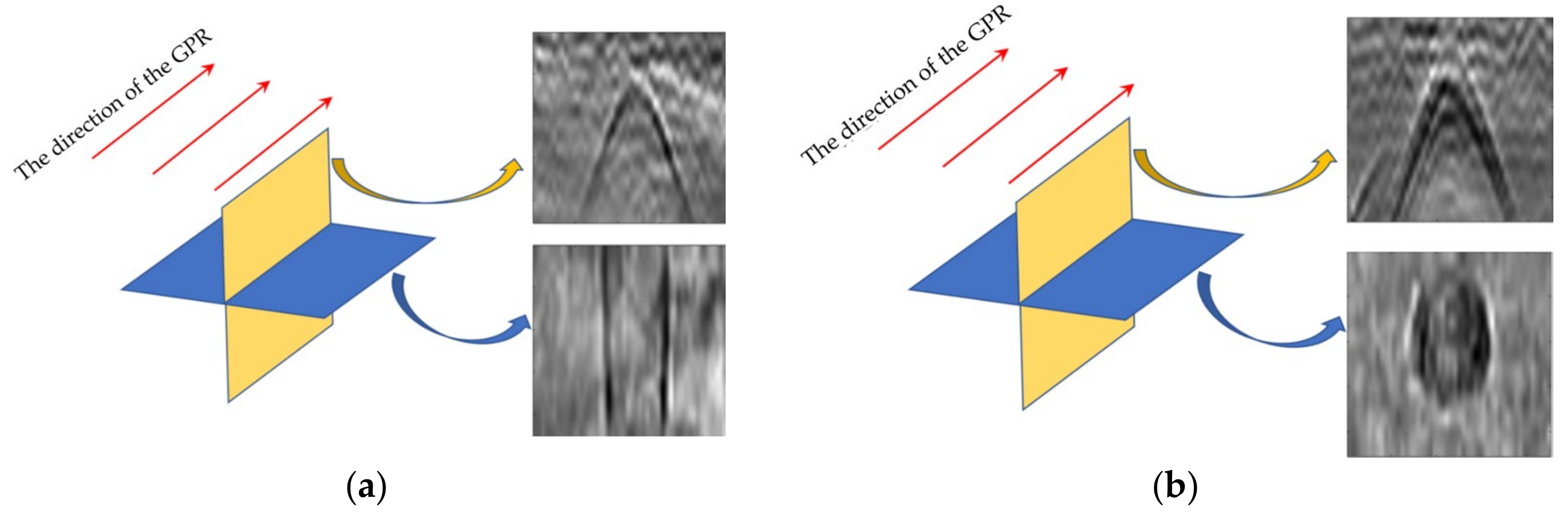
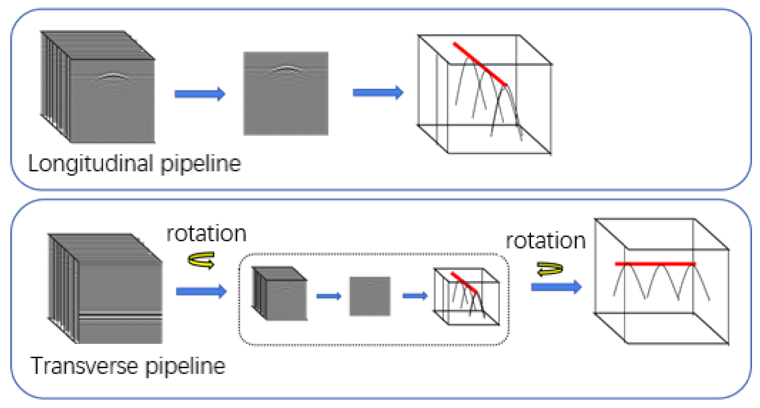
However, most of the algorithms for GPR target recognition are based on GPR B-scan images, which cannot fully reflect the characteristics of underground targets. For example, due to the influence of detection direction and image selection methods, the information in the two-dimensional B-scan image may not be recognized. As shown in Figure 1, when the surveying line direction of GPR is perpendicular to the direction of the pipeline, it is called a longitudinal pipeline (when the direction of the GPR surveying line is at an angle greater than 45° to the direction of the pipe, it is called a longitudinal line), and its B-Scan image shows a hyperbolic shape. When the surveying line direction of GPR is the same as that of the pipeline, it is called a transverse pipeline (when the direction of the GPR surveying line is at an angle less than 45° to the direction of the pipe, it is called a transverse line), and the B-Scan image of GPR does not show a hyperbolic shape but rather a straight-line shape. In addition, both underground pipelines and cavities show hyperbolic features on B-Scan images, which are difficult to distinguish, as shown in Figure 2. Therefore, to overcome the limitations of B-Scan images, it is necessary to use 3-dimensional GPR data, which can better reflect the underground structures to classify objects and obtain reliable classification results.

Deep learning has dominated the field of 2D computer vision, and its application to more complex problems, such as 3D data, is a hot trend. In recent years, researchers have made many attempts to identify 3D objects (such as RGB-D images, CAD models, 3D point cloud images, etc.). There are roughly two main directions for 3D image recognition.

One is to transform 3D to 2D by projection, multi-angle observation, image Mosaic, and other methods, in which the latest 2D target recognition method can be applied [23,24,25]. In 2019, Kang et al. [26] proposed a method for detecting underground caverns using 3-dimensional GPR data based on deep convolutional neural networks. They took advantage of a novel 2D grid image, which consists of several horizontal and longitudinal images from 3D data and conducted experimental verification by training a convolutional neural network and using real 3-dimensional GPR data obtained from urban roads in Seoul, Korea. Later, a deep learning model called UcNet was proposed in the paper [27]. Based on classification and recognition by CNN (Convolutional Neural Network) in the paper [26], UcNet selects images with detected cavities for pixel augmentation and further screening by phase analysis. The results showed that compared with traditional CNN, the misclassification of the underground cavity is significantly reduced. However, the research above did not directly deal with 3D data and instead only extracted multiple 2D images from 3D images to reflect their spatial characteristics. As a result, 3-dimensional GPR data could not be fully utilized, causing unsatisfactory classification results. Additionally, the method of 2D data input largely depends on the selection method that can represent the 2D data correlation, which is unstable.

The other is to directly take 3D data as input and directly use a 3D voxel input [28,29]. In 2020, Khudoyarov et al. proposed a method based on a 3D-CNN to directly use 3D data to classify underground targets [30]. The average accuracy of the four types of underground targets verified by real-world data was 97%. The 3D voxel image is taken as the input of the deep learning model, which can completely retain the spatial characteristics of 3D data. However, the subsequent problem is that the training of 3D-CNN is very expensive in terms of calculation, and its model size is also larger, so it is not suitable for final deployment to platforms with limited computing resources.

To make the neural network structure more lightweight, more convenient, and have less training costs in its deployment to mobile embedded devices, inspired by MobileNet [31], the neural network in this paper adopts the method of depth-wise separable convolution. Because the depth-wise separable convolution block separates the original convolution operation from the channel dimension and the space dimension, the disconnection of the information between the two dimensions will also lead to a decrease in model accuracy. Therefore, this paper increases the interaction between the channel dimension and the space dimension by integrating dimension information to improve the accuracy performance while reducing the number of parameters. Compared with the traditional 3D-CNN model, the proposed model has better advantages in terms of calculation and parameter quantity while ensuring classification performance. Meanwhile, the proposed network achieves good results with both simulated and real datasets.

This paper has four sections. In Section 1, the background and difficulties encountered in underground pipeline detection are first presented. Then we propose a deep learning network using depth-wise separable blocks with dimensional fusion to recognize 3D underground pipe targets automatically. In Section 2, the composition of a dataset is described, and then methods of data augmentation based on 3-dimensional GPR data are proposed. Section 3 shows the results of the experiment. Finally, we draw conclusions and discuss future research directions in Section 4.

2. Deep Learning Based Underground Pipeline Target Recognition Using 3-Dimensional GPR Data

In this chapter, the composition of the 3D GPR image dataset is first introduced, and then the methods of data augmentation based on the characteristics of the GPR images are proposed. Finally, the deep learning model for underground pipeline recognition is described, as well as the method to determine the position and direction of pipelines.

2.1. Real Data Acquisition and Simulation Data Generation

Due to the complexity of the collection and verification process of real 3D underground pipeline data, it is difficult to obtain a large amount of data for training. Therefore, this paper adopts the method of mixing real-world data and simulation data.

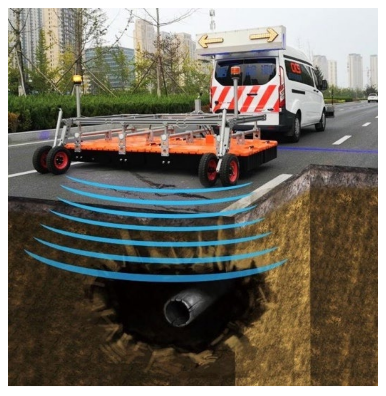
The real-world data in this paper come from the actual engineering project of Dalian Zoroy Company (Dalian, China), and the ZRY-100A vehicle-mounted 3-dimensional GPR equipment is used for data collection, whose principle is shown in Figure 3 and parameters are shown in

Table 1. The parameters of vehicle-mounted 3-dimensional GPR.

Parameters	Value
Antenna frequency	400 MHz
Pulse amplitude	50–100 V
The number of channels	36
Channel gap	0.1 m
Time window	50 ns
The number of samples	512
Measurement point interval	0.1 m

. We conduct field road detection in many cities and analyze targets such as cavities and pipelines in GPR images. The parameters of most roads are shown in

Table 2. The parameters of most roads.

Distance to the Ground Surface	Medium Type	Conductivity	Permittivity
<10 cm	Concrete	0.0005 S/m	6
>10 cm	Clay	0.001 S/m	6

. Then we intercept and classify the targets based on the experience of engineers. Finally, the accuracy of classification marks is verified by drilling and excavation on site.

In the field of GPR, GprMax is an open-source simulation software developed by a team from the University of Edinburgh in the UK, which has been updated to version 3.0. It uses the Finite Difference Time Domain (FDTD) to simulate electromagnetic wave propagation and solves Maxwell equations in three-dimensional space for forwarding simulation. It is widely used in the numerical modeling of GPR [32]. To improve the robustness of the deep learning model and expand the training set, this section uses GprMax software to generate 3-dimensional GPR echo images by setting different simulation parameters.

In the paper, a 1.2 m × 1.2 m × 1.2 m underground space is selected for simulation to generate 3-dimensional GPR images. In terms of pipelines, they can be divided into transverse and longitudinal pipelines in the general direction. For these two kinds of pipelines, the radius of the pipelines is taken as a random value in (0.02 m, 0.18 m), and the depth of the pipelines is also randomly generated as (0.3 m, 0.8 m). The medium of the pipelines can be selected as metal or PVC. In terms of cavities, spherical and cube-shaped cavities are generated randomly. The radius of spherical cavities is set as a random value in (0.05 m, 0.3 m), and their depth moves randomly within the range of (0.4 m, 0.7 m) in space. The cube void is set at the lower left of the cube starting position in (0.2 m, 0.6 m), whose length, width, and height are randomly within the range of (0.05 m, 0.3 m).

Using GprMax3.0 for 3D modeling takes more time than 2D modeling and requires higher computer performance. In view of the low efficiency of manual single simulation, there is no need to wait each time to see the completion of the simulation process, and this paper realizes the batch generation of simulation data with the help of python script combined with the original GprMax3.0 package. We entered the type and number of .in files to be generated in the python script, randomly generated the batch .in files and saved them in the corresponding folders, then called the script for batch simulation, searched for .in files in the corresponding files, and called the script for batch simulation. We then called the script of batch simulation, searched for .in files in the corresponding files, called GprMax3.0 software package module orthogonal simulation to generate the corresponding output files and images and saved them, and then stored the data in the format of a 3D matrix with the help of Numpy. In order to be close to the real data, we also randomly added a Gaussian white noise of 5 dB–30 dB; finally, the real data collected and the data generated by the simulation were tagged together to generate the .h5 dataset file, which can be used as the input of the neural network.

The simulation environment set up during the simulation is similar to the actual environment, where the medium type, conductivity, permittivity, and other parameters are the same as in Table 1. Therefore, the feature of the simulation data and real-world data are consistent. The simulation image and real-world image are shown in Figure 4.

2.2. Data Augmentation

Even though using GprMax3.0 software for genetic simulation data can obtain a large number of 3-dimensional GPR data images, only using simulation data to train the network will easily lead to poor performance in the classification of real-world data. This is in contrast to our original goal. At the same time, a convolutional neural network requires a large number of samples for training. If the training dataset is very small, it will cause many problems such as unstable network training, difficulty in reducing loss function, and overfitting of the network. Therefore, based on the simulation GPR image generated by GprMax3.0, it is necessary to further expand the real-world GPR image. Meanwhile, GprMax3.0 simulation modeling also takes a long time. To improve efficiency, the GPR images generated by simulation also need to be augmented.

The GPR image is a grayscale image, and the image is relatively monotone, so general data enhancement methods such as sharpening and brightness adjustment are not effective. In addition, the 3-dimensional GPR data format has integrity, so it is often difficult to implement 2D image augmentation. Considering the integrity of 3D data and the particularity of GPR data, we propose a method based on 3D matrix rotation to augment the data.

Three-dimensional GPR image data consist of a 3D matrix stored with a NumPy array. The point in the three-dimensional space can be represented by the normalized homogeneous coordinate [x, y, z, 1], and the transformation matrix can be used to transform the three-dimensional point into the new homogeneous coordinate system $[\widehat{x},\widehat{y},\widehat{z},1]$ during rotation transformation.

$$[x,y,z,1]\times S=[\widehat{x},\widehat{y},\widehat{z},1],$$

(1)

where S represents the transformation matrix.

When the three-dimensional matrix is rotated at a positive Angle θ around the Y-axis, there are:

$$\left\{\begin{array}{l}\widehat{x}=x\cos \theta +z\sin \theta \hfill \\ \widehat{y}=y\hfill \\ \widehat{z}=-x\sin \theta +z\cos \theta \hfill \end{array}\right.,$$

(2)

Then, S is as follows:

$$S=\left[\begin{array}{cccc}\cos \theta & 0& -\sin \theta & 0\\ 0& 1& 0& 0\\ \sin \theta & 0& \cos \theta & 0\\ 0& 0& 0& 1\end{array}\right],$$

(3)

To make the matrix rotate around the center of the image, translating the center of rotation is also required. Assuming K, M, and N are the three-dimensional dimensions of the image, respectively, then the translation matrix can be expressed as:

$$T_1=\left[\begin{array}{cccc}1& 0& 0& 0\\ 0& 1& 0& 0\\ 0& 0& 1& 0\\ -K/2& -M/2& -N/2& 1\end{array}\right],$$

(4)

We transform the coordinates back using T₂ after the rotation.

$$T_2=\left[\begin{array}{cccc}1& 0& 0& 0\\ 0& 1& 0& 0\\ 0& 0& 1& 0\\ K/2& M/2& N/2& 1\end{array}\right],$$

(5)

Finally, we can obtain:

$$[x,y,z,1]\times T_1\times S\times T_2=[\widehat{x},\widehat{y},\widehat{z},1],$$

(6)

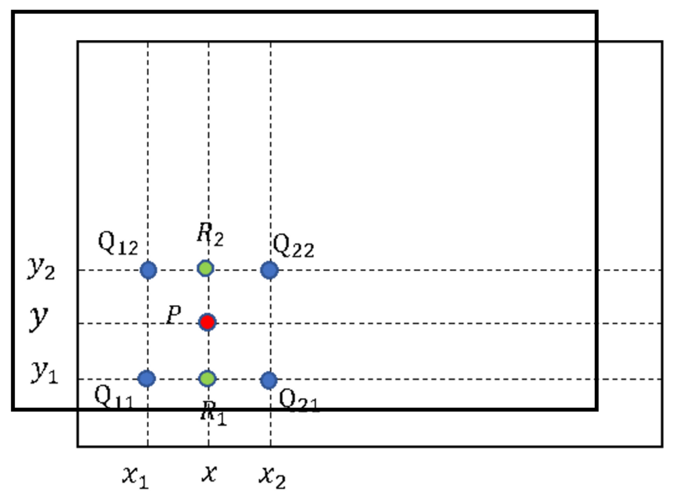
In this way, the three-dimensional image can be rotated directionally around the central position. However, because the three-dimensional dimensions K, M, and N are not equal, point mismatch will occur after directional rotation, so it is necessary to interpolate and fill the vacant positions after rotation. In this paper, we use bilinear interpolation, as shown in Figure 5, to solve this problem. First, we construct the rotated matrix, and then the corresponding value of the original matrix is found to fill in the blank by bilinear interpolation. The rotated point P can be determined using the four points Q₁₁, Q₁₂, Q₂₁, and Q₂₂ at the original position. Finally, we can obtain the pixel value of point P using Equations (7)–(9).

$$f(R_1)\approx \frac{x_2-x}{x_2-x_1}f(Q_{11})+\frac{x-x_1}{x_2-x_1}f(Q_{21}),$$

(7)

$$f(R_2)\approx \frac{x_2-x}{x_2-x_1}f(Q_{12})+\frac{x-x_1}{x_2-x_1}f(Q_{22}),$$

(8)

$$f(P)\approx \frac{y_2-y}{y_2-y_1}f(R_1)+\frac{y-y_1}{y_2-y_1}f(R_2),$$

(9)

where R₁ = (x, y₁), R₂ = (x, y₂), and f (•) is the pixel value of the point.

In addition, considering that none of the four reference points in the original position exist, to avoid introducing error features, we replace the point whose value is zero after bilinear interpolation with the GPR data value without a target. Therefore, data augmentation can be realized by rotating 3D data generated by simulation at a certain angle. It should be noted that, during the simulation of the pipeline, the augmented object selected is absolutely transverse or longitudinal in direction, and the angle range of random rotation is 0–20 degrees, which can ensure that there will be no change in transverse or longitudinal direction after rotation and no confusion in classification.

2.3. Data Preprocessing

The pre-processing of GPR data can be divided into two steps: Direct wave suppression and denoising.

For direct wave suppression, there are many methods, such as a mean filter, SVD, time threshold interception, and so on.

The mean filter method effectively suppresses the direct wave by subtracting the pixel value of each row from the mean value of that row, and the results are shown in Figure 6b,f. For the echo of the longitudinal pipeline, the hyperbolic curve is more obvious after suppressing the direct wave, but for the transverse pipeline, because its echo signal shows a horizontal straight line, the signal characteristics of the transverse pipeline are also filtered out while suppressing the direct wave. Therefore, it is inefficient to use the mean filter method to suppress the direct wave for the transverse pipeline.

The SVD method is often used to process the coherent signal, and the direct wave in the GPR B-Scan data has the largest energy and strong correlation, so the direct wave can be suppressed by the SVD method, and the results are shown in Figure 6c,g. However, while suppressing the direct waves in the transverse pipeline echo signal, it will also weaken the signal characteristics of the transverse pipeline. Therefore, the effect of suppressing the direct waves by the SVD method is also unsatisfactory.

The time threshold interception method cuts off the part of the echo data containing the direct wave directly, which does not weaken the signal characteristics of the transverse line pipeline and retains the characteristics of the hyperbola well. The results are shown in Figure 6d,h. Therefore, we choose the time threshold interception method to suppress the direct wave in this paper.

After suppressing the direct waves, there is still noise in the data, so the denoising process is still needed. In this paper, we adopt a simple and effective method based on wavelet decomposition, called the WTD method. Its specific process is shown in Figure 7. In this paper, we choose the wavelet transform using the db4 wavelet base, and the threshold value is determined according to the specific situation. Its denoising result is shown in Figure 8.

After data preprocessing, the dataset, including the transverse pipeline, the longitudinal pipeline, the underground cavity, and no target, is shown in

Table 3. Composition of the dataset after data preprocessing.

Classification Categories	Simulation Data	Real-World Data
Longitudinal pipeline	370	111
Transverse pipeline Cavity	557 315	127 97
No target	423	83

.

2.4. Deep Learning Model

2.4.1. 2.5D-CNN

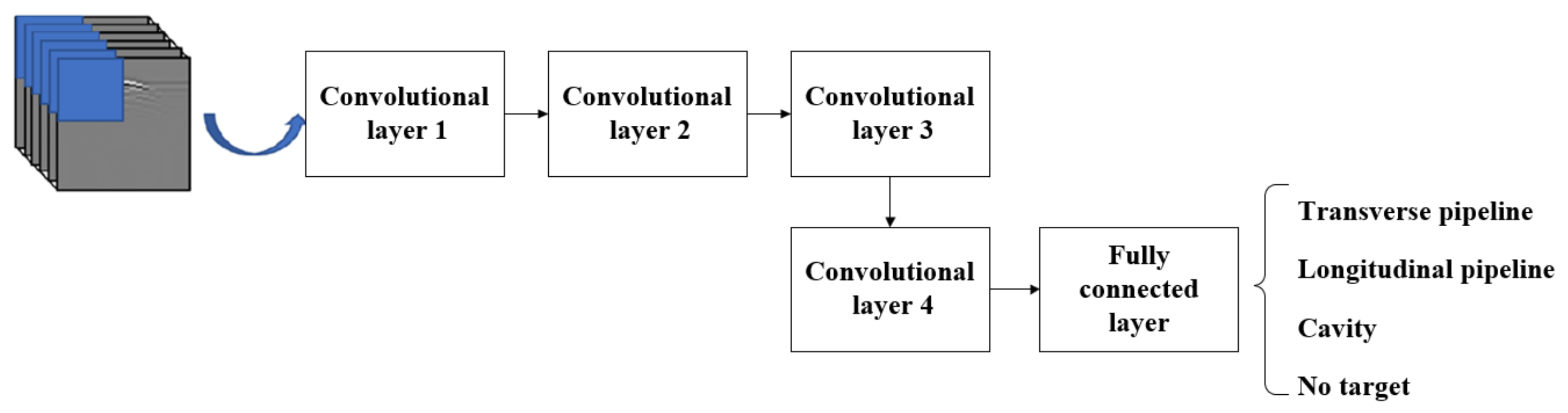
Nowadays, deep learning is developing rapidly, and various neural network structures are emerging one after another, but these structures often take 2D images as input. For three-dimensional images, in order to effectively use the mature deep learning neural network structures, the three-dimensional ground-penetrating radar data of multiple acquisition channels in parallel can be equated into multiple color channels as in the case of RGB three-channel color images, and the convolution kernels with the same depth as the channels are used for feature extraction and then accumulated in each layer, as shown in Figure 9. Since this approach still follows the pattern of 2D images for feature extraction, this approach is denoted as 2.5D-CNN to distinguish it from 2D-CNN and 3D-CNN.

In this paper, we refer to the multilayer network structure of AlexNet, which is widely used in image classification and recognition, and improve it by adapting the 2.5D-CNN neural network structure as shown in Figure 10.

A single 3D dataset with a size of (20, 40, 45) is used as the input, and the first layer of 8 (3, 3) convolution kernels is used to perform the 2D convolution operation. Then batch normalization is applied to normalize each batch of training data, and then the ReLU activation function is used to complete the nonlinear transformation of the data. The second layer is a two-dimensional convolution operation with 16 (3, 3) convolution kernels, also using batch normalization and the ReLU activation function and a (2, 2) maximum pooling operation. The third layer is a 2-D convolution operation with 32 (3, 3) convolution kernels, and the rest of the parameters and steps are the same as in the first layer. The fourth layer is a 2-D convolution operation with 64 (3, 3) convolution kernels, using the same batch normalization, ReLU activation function, and pooling as in the second layer, and a 0.2 Dropout, which randomly removes some of the hidden neurons during training to reduce training time and overfitting. The extracted features are then flattened by the Flatten layer and fed into the next layer of the fully connected network, which is output by Softmax classification.

After validation, the training hyperparameters are adjusted to a Batch Size of 10, with 10 training iterations and a learning rate of 0.0001. The previously generated dataset is used, with four classifications: A longitudinal pipeline, a transverse pipeline, an underground cavity, and no target. The training and validation sets were assigned in the ratio of 4:1, and the recognition accuracy and loss curves obtained from the iterations are shown in Figure 11. It can be seen that the accuracy and loss function gradually stabilize after four training iterations, and the training and validation results are basically consistent without any obvious overfitting.

The model parameters of 2.5D-CNN iterations of up to 10 cycles are taken to test the recognition of real data, as shown in Figure 12. For visualization, the confusion matrix of real and predicted labels is represented in the form of a heat map, and the four classifications (longitudinal pipeline, transverse pipeline, void, and no target) are replaced by labels 0 to 3, respectively. It can be seen that there are 18 misclassifications among 416 data samples. Four samples of classification 0 (longitudinal pipeline) are misidentified as classification 1 (transverse pipeline) and one sample is misidentified as classification 3 (void); six samples of classification 3 (void) are misidentified as classification 0 (longitudinal pipeline) and seven samples are misidentified as classification 1 (transverse pipeline).

2.4.2. 3D-CNN

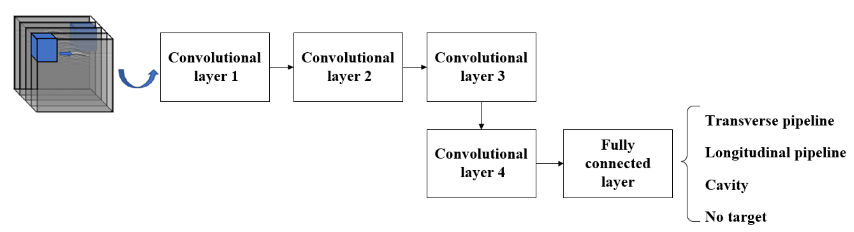
Three-dimensional convolutional neural networks (3D-CNN) are primarily used in the video field for classification and action recognition at the beginning, and feature extraction of inter-frame motion information in the temporal dimension can be performed with the help of 3D convolutional kernels. The 3D data structure of the array ground-penetrating radar is actually similar to that of video frames, except that it corresponds from temporal to spatial information. In this subsection, 3D-CNN is applied to the 3D image pipeline recognition of array ground-penetrating radar to overcome the disadvantage that a 2D convolutional neural network is not sensitive enough to spatial information.

To facilitate a comparison with 2.5D-CNN and subsequent neural network structures, the convolutional neural network structure used in this paper is not changed and still includes four convolutional layers and one fully connected layer, as shown in Figure 13. In the 3D-CNN, the single input format is (20, 40, 45, 1), the 3D convolutional operation is performed by the 3D convolutional kernels of (3, 3, 3), and the pooling operation is performed by the maximum pooling of (2, 2, 2) on the 3D scale. Other structural parameters such as the number of convolutional kernels in each layer and the distribution of processing units in each layer are the same as in the 2.5DCNN. The accuracy curves and convergence curves of the training and validation obtained by 3D-CNN without changing the training hyperparameters are shown in Figure 14. By using Dropout and batch normalization during training and keeping more parameters during validation, it can be seen that the recognition accuracy of the validation set is close to 100% by the third cycle of iteration, and the loss function is basically stable in the following cycles. With the current dataset, the 3D-CNN can complete the training of the model after approximately three iterations.

Using real data as the test, we can obtain the heat map of classification recognition, and as shown in Figure 15, we can see that all four real samples are basically classified correctly, and only one sample is classified incorrectly. The convergence ability and recognition accuracy of the 3D-CNN model are better than 2.5D-CNN with the same network structure, which shows the advantage of 3D-CNN in processing and analyzing 3D data. However, the 3D-CNN, which introduces one more dimension, also requires more neural network parameters and a longer training duration than the 2.5D-CNN. The 3D-CNN used in this section contains 102,068 parameters, of which 101,828 are trainable, while the 2.5D-CNN contains 31,620 parameters, of which 31,380 are trainable. It can be seen that the neural network parameters of the 3D-CNN are more than three times those of the 2.5D-CNN, and the difference in network parameters between the 3D-CNN and the 2.5D-CNN is even greater when the network contains more fully connected layers.

2.4.3. CNN + RNN

Both the 2.5D-CNN and the 3D-CNN used above directly input the 3D data image as a whole into the neural network. The 2.5D-CNN does not perform well due to the lack of accuracy in spatial information extraction, while the 3D-CNN requires a large number of parameters and increases in complexity in order to extract more spatial features.

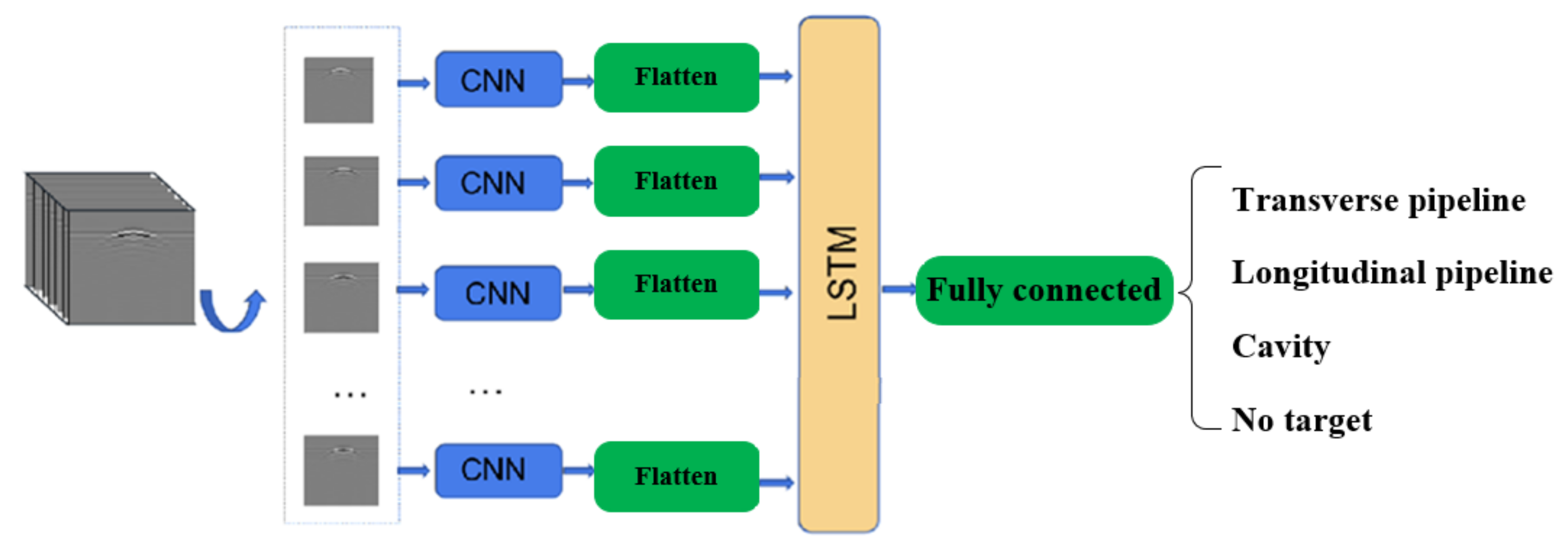
In this subsection, we adopt another way of thinking and consider using the correlation between 2D images in 3D data images to classify and recognize 3D data images, for which the combination of a convolutional neural network and a recurrent neural network, i.e., CNN + RNN, is used. The network structure is shown in Figure 16. The CNN is first used to extract features from each 2D image of the 3D image, and then these features are integrated and fed into the RNN network to process these features, and finally, the target object is classified and recognized. In the RNN part, a single-layer LSTM network is used. Since the number of LSTM parameters is four times higher than the number of CNN parameters with the same number of inputs and outputs, the output of the CNN network structure in the last two subsections is directly spanned by the Flatten layer and fed into the LSTM network, which generates a large number of parameters that are not worth the loss. The dimension of the hidden unit of the RNN part of the LSTM network is taken as 36, which corresponds to the output of the fully connected part of the Softmax classification connected to four nodes.

The accuracy curves and convergence curves of the training and validation obtained by the CNN + RNN approach without changing the hyperparameters are shown in Figure 17. The confusion matrix heat map obtained from the test set is shown in Figure 18.

2.4.4. Analysis of Performance

In order to comprehensively test the classification ability of neural networks, considering the different number of samples for each classification, this subsection will compare three neural network algorithms with accuracy, precision, recall, and F1 value as evaluation indexes, and also add the number of parameters as evaluation indexes to measure the complexity of each algorithm. The results are shown in

Table 4. Evaluation index values for each algorithm classification test.

Evaluation Indicators	2.5D-CNN	3D-CNN	CNN + RNN
Accuracy	0.9567	0.9976	0.9735
Precision	0.9636	0.9975	0.9719
Recall	0.9561	0.9977	0.9702
F1	0.9585	0.9976	0.9702
Number of parameters	40,572	102,068	56,880
Training time	20.338 s	104.797 s	37.416 s

.

We can see that 3D-CNN has better performance in terms of accuracy, precision, recall, and F1 value, but it requires the most parameters, and the number of parameters is more than twice that of 2.5D-CNN, so determining how to reduce the number of parameters in the 3D-CNN is a direction worth studying. However, in embedded devices such as FPGAs, it is difficult to achieve parallel acceleration and optimization because the RNN part needs to rely on before and after information. While the 2.5D-CNN is not very good at classification, the number of parameters is small and can be accelerated and optimized by FPGAs. It can be considered when resources are tight and speed is required.

2.5. Improved 3D-CNN Model

When using the 3D-CNN model to directly process 3D data, if a 3D voxel image is taken as the input of the deep learning model, the spatial characteristics of 3D data can be completely retained. However, the subsequent problem is that the training cost is very expensive in terms of calculation, and the model size is also large, so it is not suitable for final deployment to platforms with limited computing resources.

The depth-wise separable convolution block includes the depth-wise part and the point-wise part. The depth-wise convolution block is mostly used in the lightweight improvement of two-dimensional neural networks. Similarly, the 3D convolution kernel will significantly increase the amount of calculation, which requires an effective method to reduce the amount of calculation. Therefore, this paper extends the depth-separable convolution block to the lightweight improvement of the 3D neural network.

For the 3D-CNN, W, H, L, and C are used to represent the three-dimensional dimensions and the channel number of the input feature tensor, respectively, and K represents the size of the convolution kernel. Then, for a 3D convolution operation, the input feature is W × H × L × C_in and the output feature is W × H × L × C_out. The traditional convolution operation can be divided into C_in depth-wise processes of K × K × K × 1 and C_out point-wise processes of 1 × 1 × 1 × C_in by using a depth-wise separable convolution block. The number of network parameters is used to represent the amount of calculation, so the amount of calculation of traditional convolution is C_out × K × K × K × Cin × W × H × L, that of the depth-wise part is K × K × K × C_in × W × H × L, and that of the point-wise part is 1 × 1 × 1 × C_in ×C_out ×W × H × L. The relationship between the amount of calculation is as follows:

$$\frac{(K\times K\times K\times C_{in}\times W\times H\times L)+(C_{in}\times C_{out}\times W\times H\times L)}{K\times K\times K\times C_{in}\times C_{out}\times W\times H\times L}=\frac{1}{C_{out}}+\frac{1}{K\times K\times K},$$

(10)

Therefore, with the help of the 3D depth-separable convolution block, the parameters and calculation of 3D convolution operation are reduced.

However, the depth-wise separable convolution block separates the traditional convolution operation from the channel dimension and the space dimension. While reducing the number of parameters, it also reduces the connection of the dimension information, which will lead to a decline in classification accuracy. Therefore, by integrating dimension information, we can increase the interaction between the channel dimension and the space dimension to improve the accuracy of performance.

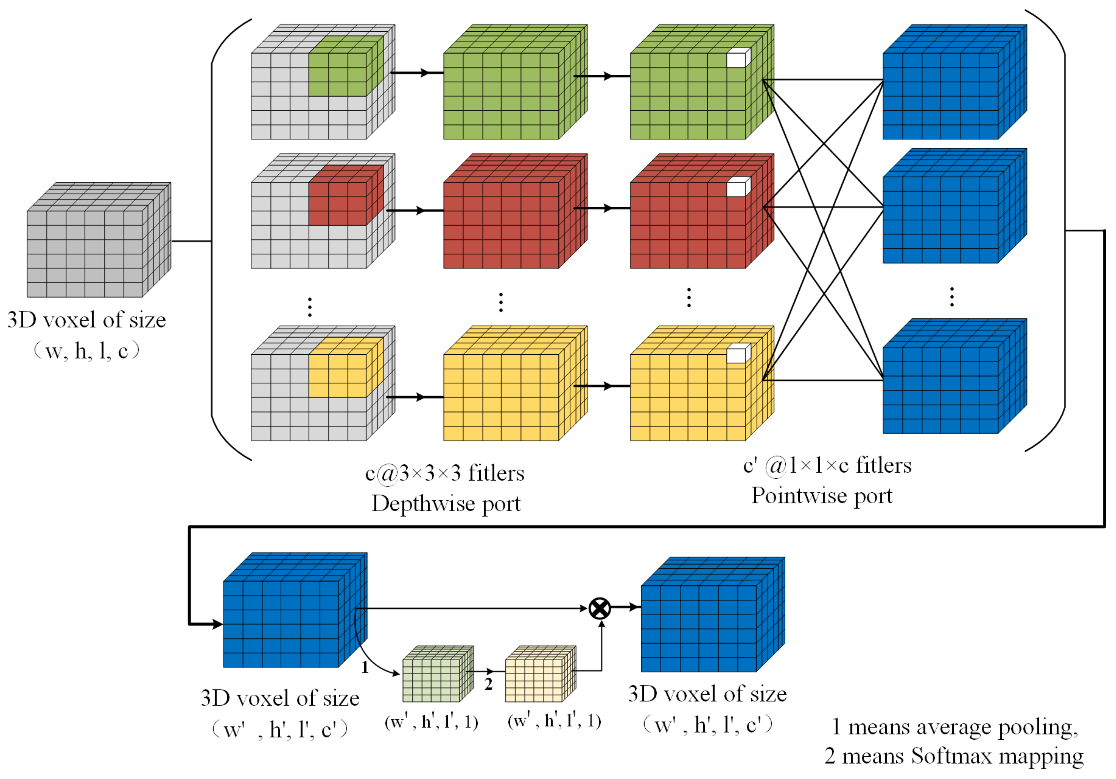
This paper proposes an improved depth-wise separable convolution block whose structure is shown in Figure 19, shows the number of channels before @ and the size of the convolution kernel after @. First, on the original basis, a dimension fusion module is added before Batch Normalization. Second, in the dimension fusion module, the pooling layer is used to average the corresponding positions of data for different channels, and then using SoftMax to process the data, it maps the data in the interval of (0, 1) and multiplies the data from different channels to obtain the data after dimension fusion. Finally, the steps following the original depth-wise separable convolution block are performed successively.

$${\mathrm{U}}_{DF}=\alpha \ast U_i,$$

(11)

$$\alpha =Softmax\left(\frac{1}{C_{in}}{\displaystyle \sum _{i=1}^{C_{in}}{f}_{WHL}(i)}\right),$$

(12)

where C_in is the number of channels and f_WHL (i) and U_i are the data of the i^th channel.

The paper refers to and adjusts AlexNet’s multi-layer network structure [12], which is widely used in image classification and recognition. We apply the improved depth-wise separable convolution block to the AlexNet network model. The whole network structure model is shown in Figure 20. Figure 20 shows the number of channels before @ and the data size after @.

2.6. Determination of Pipeline Position and Direction

In practical applications, it is often necessary not only to know whether there is a pipeline target in the GPR image but also to know the specific position and direction of the pipeline. Therefore, we propose a pipeline-positioning scheme.

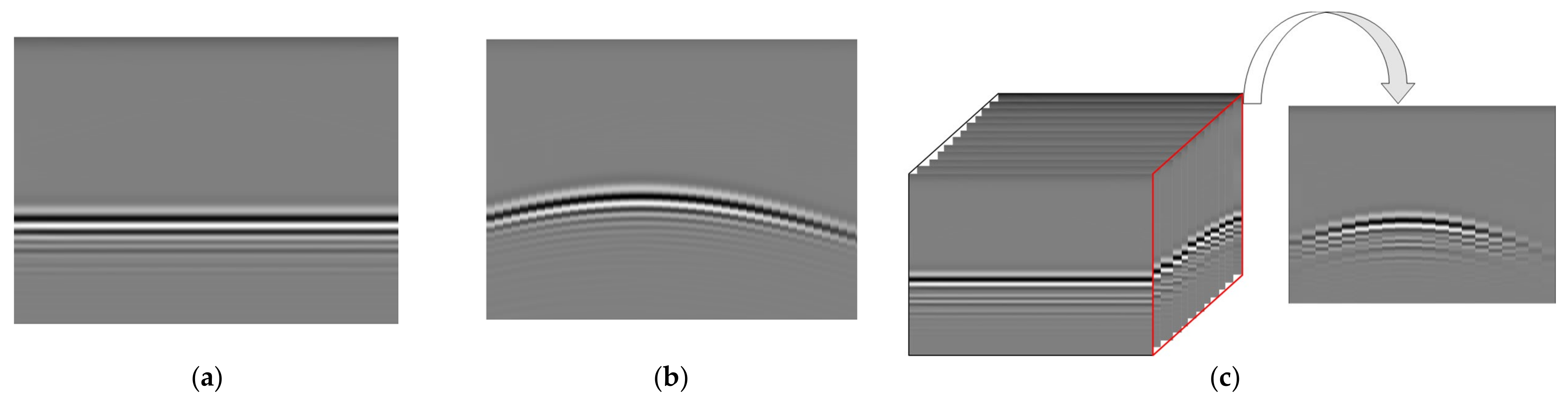
In the paper, the pipeline target is divided into two types: A transverse pipeline and a longitudinal pipeline. Three-dimensional GPR data can be regarded as the combination of B-Scans of multiple channels. Therefore, during pipeline positioning, a B-Scan can be used for positioning, and the pipeline positioning can be realized by extracting the vertices of the hyperbola, and then the position and direction of the pipeline in 3D space can be obtained by connecting the positions of vertices in multiple B-Scans. It should be noted that for the horizontal pipeline because the hyperbola is on the 2D B-Scan in the direction of the GPR array, it needs to be rotated before processing, as shown in Figure 21. The red line in Figure 21 shows the line at the apex of the hyperbola.

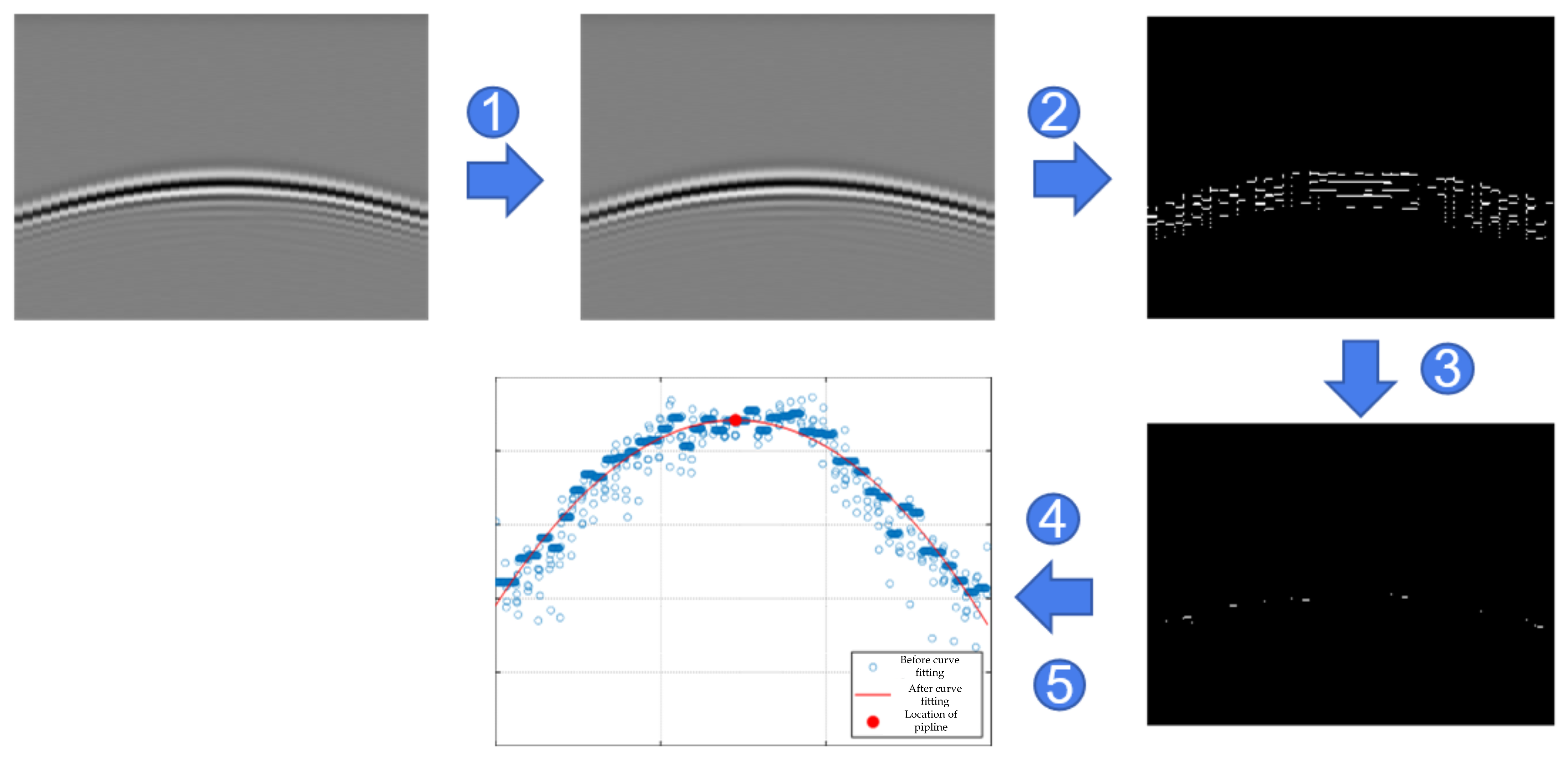
The extraction of hyperbolic vertices in B-Scan images is the most important step to determine the pipeline location and direction in 3D space. Therefore, we propose a pipeline location scheme based on the Canny operator conic curve fitting method. Figure 22 shows the processing of the simulated B-Scan, and the specific steps corresponding to the numbers in the figure are as follows:

• The B-Scan image is processed by median filtering to remove the impulse noise and protect the signal edge from being blurred.
• The canny operator is used for edge detection. The canny operator is a very effective and adaptable algorithm in the field of edge detection. It can adjust parameters to identify different edges according to different application requirements and has the advantages of a low error rate and accurate edge positioning. A Gaussian filter is first used for smoothing and filtering. Then the gradient and gradient direction is found, and non-maximal value suppression is used to refine the edges. Finally, isolated low-threshold points are suppressed, and edges are connected using double-threshold detection and connectivity detection.
• Trade-offs are made based on edge cases. In the case of multiple edge points in the same column, coordinate averaging is used to calculate the average. In addition, the edge points obtained by the Canny operator may be discontinuous, so the points whose height difference exceeds the threshold are discarded and replaced by a row of edge points.
• Regarding curve fitting, each pixel is scanned line by line, and we record the coordinates and number of white points (value 1) and use the quadratic function to perform curve-fitting on the edge points after processing.
• For vertex determination, the derivative of the fitted quadratic curve is obtained, and the points where the derivative is 0 are marked and the horizontal and vertical coordinates are recorded.

3. Results

3.1. Dataset Setup and Experimental Setup

We use the data generated in Section 2.2 as the experimental dataset, which consists of the longitudinal pipeline, the transverse pipeline, the underground cavity, and no target, as shown in Table 3. Three-dimensional GPR image data are trimmed to 20 × 40 × 45 (channel, height, and width). The proportion of the training set and verification set is 4:1.

In order to evaluate the performance of the proposed CNN model, this paper uses multiple control groups and compares the classification results with those of each control group with the same network structure and training method.

The first control group is the 2D-CNN. AlexNet has been developed for the general classification of RGB images. Therefore, for 3-dimensional GPR images, the data of multiple acquisition channels can be equivalent to multiple color channels and sent into a 2D-CNN network, similar to processing RGB three-channel color images. The second control group is a CNN using the traditional 3D convolution kernel, denoted as 3D-CNN. The third control group is a CNN using the 3D depth-wise separable convolution block, denoted as DS-3D-CNN. The last group is a CNN with 3D depth-separable convolution blocks with dimension fusion proposed in this paper, denoted as DF-DS-3D-CNN.

3.2. Classification Results

The classification performance of the proposed method and the other three control algorithms is compared using the generated training set. Under the condition that the hyperparameters remain the same, the comparison figure of the accuracy curve and loss function curve obtained by iteration is shown in Figure 23. The evaluation indexes of each model obtained through the test set are shown in

Table 5. Training set and test set of convolutional neural network.

Classification Category	Longitudinal Pipeline		Transverse Pipeline		Cavity		No Target
	Training	Testing	Training	Testing	Training	Testing	Training	Testing
number of 3D GPR images	371	110	558	126	332	80	406	100

. For an intuitive representation, the confusion matrix of true and predicted labels is represented as a heat map, and the four classifications (vertical pipeline, horizontal pipeline, void, and no target) are replaced by labels 0 to 3, respectively, as shown in Figure 24.

In Figure 24a, the classification performance of the traditional 2D-CNN is the weakest, and 18 of the 416 data samples are misclassified, while the 3D-CNN has the strongest classification performance, and only 1 sample is assigned to the wrong category. Therefore, the 3D-CNN has great strength in processing and analyzing 3-dimensional GPR data. However, compared with the 2D-CNN, the 3D-CNN requires more neural network parameters and a longer training time because of an extra dimension. In

Table 6. Evaluation index values for the classification performance of each algorithm.

Evaluation Indicators	2.5D-CNN	3D-CNN	DS-3D-CNN	DF-DS-3D-CNN
Accuracy	0.9567	0.9976	0.9756	0.9880
Precision	0.9636	0.9975	0.9768	0.9898
Recall	0.9561	0.9561	0.9769	0.9886
F1-Measure	0.9585	0.9585	0.9767	0.9890
parameters	40,572	102,068	33,804	33,804
Training time	20.338 s	104.797 s	195.189 s	254.886 s

, the neural network parameters of the 3D-CNN are three times more than those of the 2D-CNN. When the network contains more fully connected layers, the difference in network parameters between the 3D-CNN and the 2D-CNN will be more significant.

In Figure 23, the DS-3D-CNN has worse convergence performance and accuracy than the 3D-CNN. However, the DS-3D-CNN has 33,804 parameters, which are significantly fewer than those of the 3D-CNN with 102,068 parameters by 66.9%. Although the reduction of the calculation amount also leads to a decline in accuracy, compared with the 2D-CNN, which has 40,572 parameters, the DS-3D-CNN has better accuracy performance and convergence performance with fewer parameters. The experimental results demonstrate the feasibility of replacing the original 2D neural network and 3D neural network with depth-wise separable convolution.

The dimensional information will be separated while the DS-3D-CNN reduces the parameters. In contrast, the DF-DS-3D-CNN proposed in this paper increases the interactivity of channel dimension and space dimension using dimensional information fusion. Though the DF-DS-3D-CNN has the same number of parameters as the DS-3D-CNN and only increases the small amount of calculation brought by average pooling and SoftMax operation, it can efficiently improve the classification and recognition ability of the network model. The classification results illustrate that the algorithm can not only reduce the number of parameters by 66.9% compared with the 3D-CNN but can also maintain a recognition accuracy that differs from the 3D-CNN by less than 1%. Furthermore, although the training time of the DF-DS-3D-CNN network is longer, since the network trained in advance can be used for detection, the training time is not particularly important.

4. Discussion and Conclusions

In this paper, we proposed a method based on deep learning for underground pipe detection using 3-dimensional GPR images. First, this paper proposes a three-dimensional matrix rotation to augment the 3-dimensional GPR data and constructs the dataset, which may be the first dataset in the field of GPR, after data preprocessing. Second, this paper illustrates the advantages of the 3D-CNN compared with the 2D-CNN in underground pipe recognition. Furthermore, to solve the problems of excessive calculation and parameters in the 3D-CNN, this paper proposes a structure of depth-separable convolutional blocks with the dimensional fusion module. By adding this structure, the number of network parameters is reduced by 66.9% while its performance is similar to that of the 3D-CNN in the underground pipeline classification task, which provides a foundation for the future deployment of the model to mobile platforms with limited computing resources. Finally, this paper proposes a curve-fitting method based on the Canny operator to find the position of the pipe by detecting hyperbolic vertices in B-Scan and then finding the direction of the pipe in 3D space.

There are still some shortcomings in the present study. For example, the real data are limited, and the simulation data cannot represent the real measurement results well. Different cities may have different image characteristics when the difference in local media is large. For future work, we will acquire more real-world data and build a more complete dataset where we can more accurately verify the performance of the network proposed in this paper. We will also acquire data from more cities to improve the generalization ability of the network. We also plan to find a suitable semi-supervised method to decrease the difficulty of manual annotation of 3-dimensional GPR images. In order to better prevent possible hazards and identify changes in the underground environment, we will try to propose an algorithm to compare the similarity of the data of the same section of highway detected at different times and obtain the difference between them. Meanwhile, we will try to deploy the network to mobile platforms such as FPGA in the future to achieve real-time detection of underground targets.