
Overview on Intrusion Detection Systems Design Exploiting Machine Learning for Networking Cybersecurity

 ,
,  ,
, 

 and
and
Abstract
:1. Introduction
1.1. Overview
1.2. Motivations
1.3. Machine Learning in Network Security
- Threat detection: Machine learning can be used to develop predictive models capable of identifying and detecting suspicious behavior or cyber attacks in communication networks. These models can analyze large amounts of data in real time from various sources, such as network logs, packet traffic and user behavior, in order to identify anomalies and patterns associated with malicious activity.
- Automation of attack responses: Automation is a key aspect in the security of communication networks. Using machine learning algorithms can help automate an attack response, allowing you to react quickly and effectively to threats. For example, a machine learning system can be trained to recognize certain types of attacks and automatically trigger appropriate countermeasures, such as isolating compromised devices or changing security rules.
- Detect new types of attacks: As cyberthreats evolve, new types of attacks are constantly emerging. The traditional signature-based approach may not be enough to detect these new threats. The use of machine learning algorithms can help recognize anomalous patterns or behavior that could indicate the emergence of new types of attacks, even in the absence of specific signatures.
- Reduce False Positives: Traditional security systems often generate large numbers of false positives, that is, they falsely report normal activity as an attack. This can lead to wasted time and valuable resources in dealing with non-relevant reports. Using machine learning models can help reduce false positives, increasing the efficiency of security operations and enabling more accurate identification of real threats.
- Adaptation and continuous learning: Machine learning models can be adapted and updated in real time to address new threats and changing conditions of communication networks. With continuous learning, models can improve over time, gaining greater knowledge of threats and their variants.
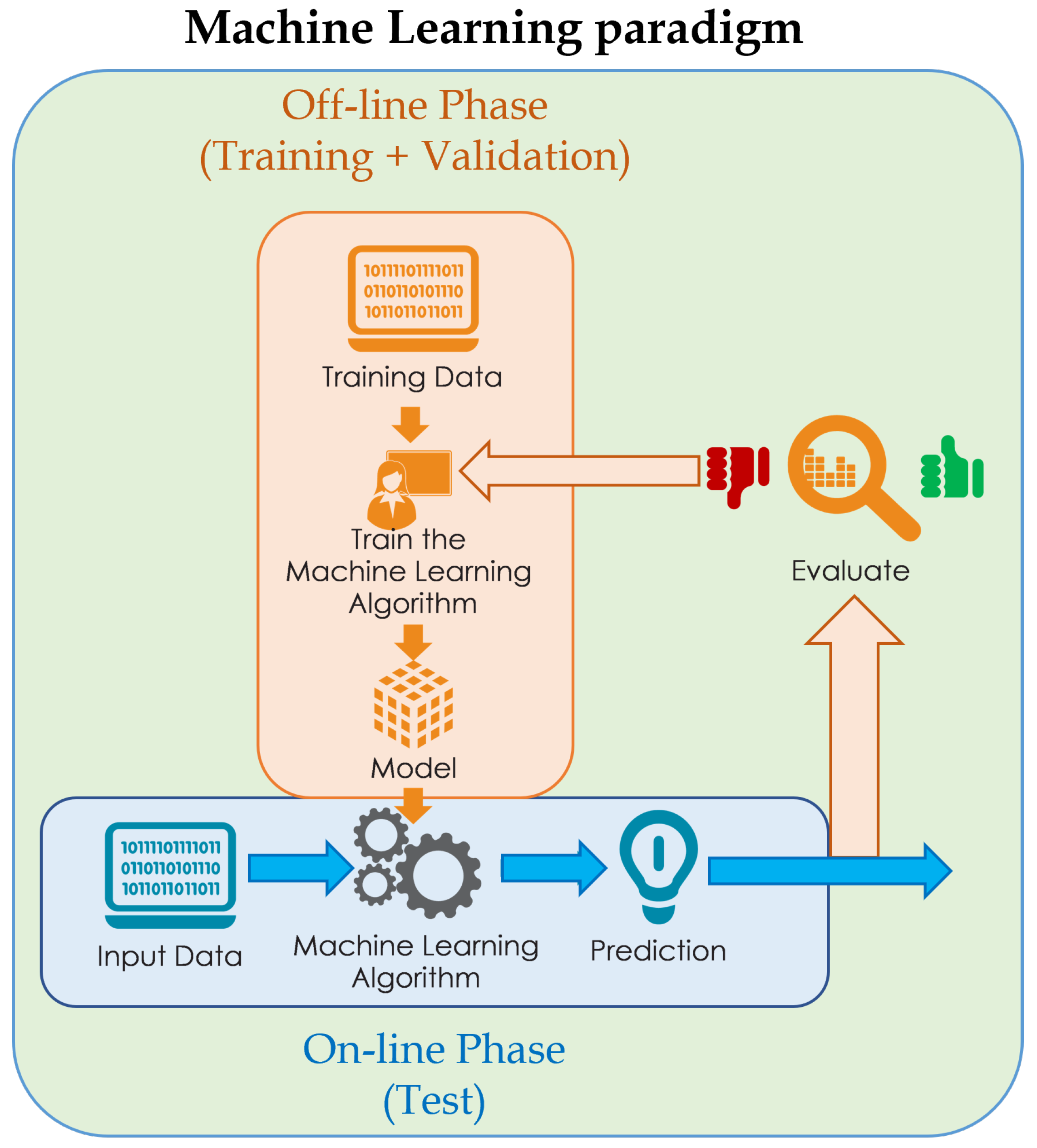
- Data Collection: The initial phase involves the collection of training data. This data consists of labeled examples, i.e., pairs of matching inputs and outputs. For example, if we are trying to build a model to recognize images of cats, the data will contain images of cats labeled “cat” and different images labeled “not cat”.
- Data preparation: This phase involves cleaning, normalizing, and transforming the training data to make it suitable for processing by the machine learning model. This can include eliminating missing data, handling categorical characteristics, and normalizing numeric values.
- Model selection and training: In this phase, you select the appropriate machine learning model for the problem at hand. The model is then trained on the training data, which consists of making the model learn the patterns and relationships present in the data. During training, the model is iteratively adjusted to minimize the error between its predictions and the corresponding output labels in the training data.
- Model Evaluation: After training, the model is evaluated using separate test data, which was not used during the training. This allows you to evaluate the effectiveness of the model in generalizing patterns to new data. Several metrics, such as accuracy, precision, and area under the ROC curve, are used to evaluate model performance.
- Model Usage: Once the model has been trained and evaluated, it can be used to make predictions on new input data. The model applies the relationships learned during training to make predictions about new input instances.
1.4. Contribution
- A thorough analysis of multiple machine learning algorithms has been conducted to effectively handle the processing of large volumes of network traffic data. These algorithms can be scaled to accommodate the expanding sizes of networks, resulting in the development of a robust and efficient intrusion detection system.
- The impact of dataset selection on the performance of intrusion detection systems has been explored in this study. By comparing the performance of intrusion detection systems across three distinct datasets (KDD 99, UNSW-NB15, and CSE-CIC-IDS 2018), a better understanding of the influence of dataset choice on system performance has been achieved.
- This research has made significant contributions to the advancement of effective feature engineering techniques, which are essential for constructing successful machine learning models. These techniques encompass feature selection, feature scaling, and feature normalization, enhancing the overall effectiveness of the models.
- Additionally, this study proposes an analysis of the computational time required by different models, a factor often overlooked in existing literature. This inclusion enriches the performance analysis of the models across the selected datasets.
2. Related Works
2.1. Support Vector Machine
2.2. Decision Tree
2.3. Random Forest
- 1
- Bootstrapped Sampling: Random Forest starts by creating multiple subsets of the original training data through bootstrapped sampling. This sampling technique involves randomly selecting data points from the original dataset with replacement. Each subset is called a bootstrap sample and is used to train a separate decision tree;
- 2
- Random Feature Selection: For each decision tree in the Random Forest, a random subset of features is selected. This process introduces randomness and reduces the correlation between trees. The number of features in the subset is typically determined by a hyper-parameter called “max_features”.
- 3
- Decision Tree Construction: Using the bootstrapped sample and the randomly selected feature subset, a decision tree is constructed for each subset. The construction follows the same steps as in the standalone decision tree learning process, including attribute selection, splitting, and recursive construction;
- 4
- Voting or Averaging: Once all the decision trees are constructed, predictions are made by either voting (for classification tasks) or averaging (for regression tasks) the predictions of individual trees. In classification tasks, the class with the highest number of votes is chosen as the final prediction. In regression tasks, the mean or median value of the predictions is taken as the final prediction.
2.4. Linear Discriminant Analysis
- Data Preprocessing: LDA requires a training dataset with predefined classes. The training dataset consists of feature vectors X and their corresponding class labels y;
- Class-wise Summary Statistics: For each class in the training dataset, LDA computes class-specific summary statistics. These statistics include the mean vector and the covariance matrix of the features within each class;
- Between-class Scatter Matrix: LDA computes the between-class scatter matrix (), which measures the separation between different classes. It is defined as the sum of the outer products of the difference between class means and the overall mean, weighted by the number of samples in each class.where is the number of samples in class i, is the mean vector of class i, mu is the overall mean vector.
- Within-class Scatter Matrix: LDA computes the within-class scatter matrix (SW), which measures the spread of the samples within each class. It is defined as the sum of the covariance matrices of each class, weighted by the number of samples in each class.where is the covariance matrix of class i.
- Fisher’s Criterion: LDA aims to find a projection that maximizes the separation between classes while minimizing the scatter within each class. This is achieved by computing Fisher’s criterion, which is the ratio of the determinant of SB to the determinant of SW.where w is the projection vector.
- Projection Vector: To find the optimal projection vector w, LDA solves the generalized eigenvalue problem:where is the eigenvalue corresponding to w.
- Dimensional Reduction: LDA selects the top k eigenvectors corresponding to the largest eigenvalues as the projection vectors. These projection vectors form a lower-dimensional subspace that preserves the most discriminating information between classes.
- Classification: To classify a new observation, LDA projects it onto the subspace spanned by the projection vectors and assigns it to the class with the closest mean in the projected space.
2.5. K-Nearest Neighbors
- Data Preparation: The training dataset consists of labeled examples, where each example is represented by a feature vector X and its corresponding class label y.
- Choosing the Value of k: The value of k, representing the number of nearest neighbors to consider, needs to be determined. Typically, k is chosen based on domain knowledge or through cross-validation.
- Computing Distance: KNN utilizes a distance metric, such as Euclidean distance or Manhattan distance, to measure the similarity between feature vectors. Lets denote the distance metric as , where and are two feature vectors.
- Finding K Nearest Neighbors: Given an input data point x, the distances between x and all data points in the training set are computed. The k nearest neighbors of x are selected based on the smallest computed distances. Lets denote the set of k nearest neighbors as .
- Voting or Averaging: For classification tasks, KNN employs majority voting to determine the class label of the input data point. It assigns the class label that is most frequent among the class labels of the k nearest neighbors in . Mathematically, the predicted class label for x, denoted as , is given by:where represents the class label of the ith neighbor in , is the indicator function, and returns the class label with the highest count. For regression tasks, KNN takes the average of the target values of the k nearest neighbors to make a prediction. Mathematically, the predicted value for x, denoted as , is given by:where represents the target value of the ith neighbor in .
- Handling Ties: In cases where there is a tie in the number of votes for different classes during majority voting, various strategies can be employed. For example, KNN may select the class label of the nearest neighbor among the ties or use weighted voting based on the distances.
- Predicting with the Trained Model: Once the KNN model is trained on the training dataset, it can be used to make predictions on new, unseen data points by following the steps mentioned above.
2.6. Artificial Neural Network
3. Selected Datasets
3.1. KDD 99
3.2. UNSW-NB15
3.3. CSE-CIC-IDS 2018
4. ML Performance Evaluation
4.1. Binary Classification Metric
- TP (true positive): if the model predicts Norm, it is also the correct answer.
- FP (false positive): if the model predicts Norm, the correct answer is Att.
- TN (true negative): if the model predicts Att, and it is also the correct answer
- FN (false negative): if the model predicts Att, the correct answer is Norm.
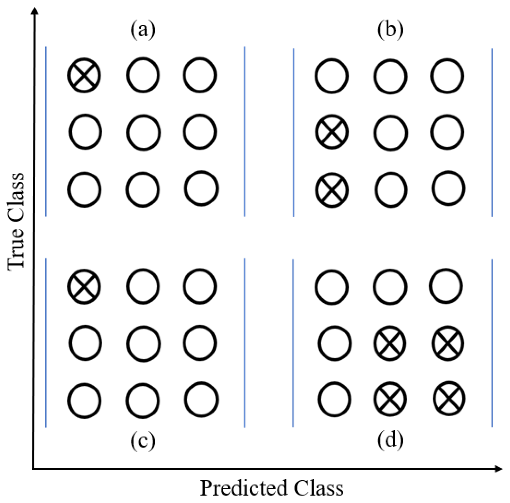
4.2. Multi-Class Classification Metric
- Macro-average: This method simply calculates the average of the binary metrics, assigning equal weight to each class. It can be particularly useful when infrequent classes hold significance, as it highlights their performance. With the Macro-average, the effect of the most frequent classes is considered equally important as that of the least frequent ones.
- Micro-average: In this approach, each sample-class pair contributes equally to the overall metric. Instead of summing the metrics by class, it sums the numerators and denominators that constitute the metrics by class to calculate an overall quotient. The Micro-average is often preferred in multi-label or multi-class classification settings, where the majority class must not dominate the evaluation.
5. Dataset Manipulation
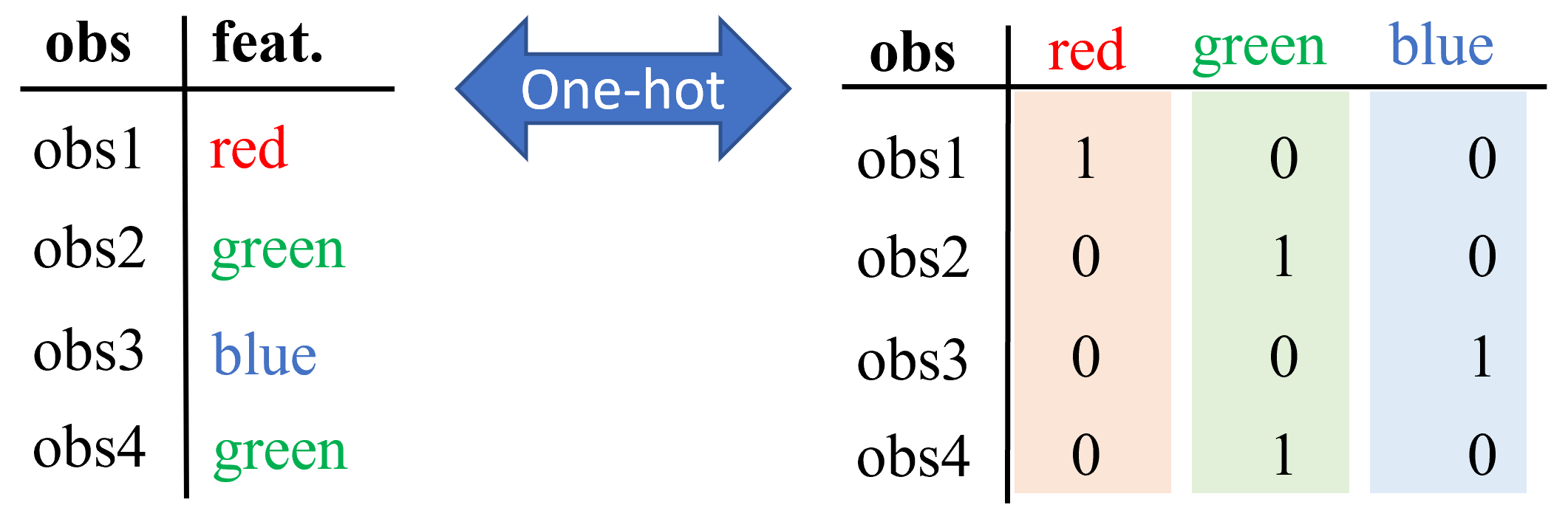
5.1. Variable Encoding
5.2. Data Scaling
5.3. Dataset Balancing
6. Experimental Design and Results
7. Final Discussion
8. Conclusions and Future Work
Author Contributions
Funding
Institutional Review Board Statement
Informed Consent Statement
Data Availability Statement
Conflicts of Interest
References
- Musa, U.S.; Chhabra, M.; Ali, A.; Kaur, M. Intrusion Detection System using Machine Learning Techniques: A Review. In Proceedings of the 2020 International Conference on Smart Electronics and Communication (ICOSEC), Trichy, India, 10–12 September 2020; pp. 149–155. [Google Scholar]
- Aljabri, M.; Altamimi, H.S.; Albelali, S.A.; Maimunah, A.H.; Alhuraib, H.T.; Alotaibi, N.K.; Alahmadi, A.A.; Alhaidari, F.; Mohammad, R.M.A.; Salah, K. Detecting malicious URLs using machine learning techniques: Review and research directions. IEEE Access 2022, 10, 121395–121417. [Google Scholar] [CrossRef]
- Okey, O.D.; Maidin, S.S.; Adasme, P.; Lopes Rosa, R.; Saadi, M.; Carrillo Melgarejo, D.; Zegarra Rodríguez, D. BoostedEnML: Efficient technique for detecting cyberattacks in IoT systems using boosted ensemble machine learning. Sensors 2022, 22, 7409. [Google Scholar] [CrossRef] [PubMed]
- Htun, H.H.; Biehl, M.; Petkov, N. Survey of feature selection and extraction techniques for stock market prediction. Financ. Innov. 2023, 9, 26. [Google Scholar] [CrossRef] [PubMed]
- Bhuyan, M.H.; Bhattacharyya, D.K.; Kalita, J.K. Network Traffic Anomaly Detection and Prevention: Concepts, Techniques, and Tools; Springer: Berlin/Heidelberg, Germany, 2017. [Google Scholar]
- Liu, J.; Dong, Y.; Zha, L.; Tian, E.; Xie, X. Event-based security tracking control for networked control systems against stochastic cyber-attacks. Inf. Sci. 2022, 612, 306–321. [Google Scholar] [CrossRef]
- Zha, L.; Liao, R.; Liu, J.; Xie, X.; Tian, E.; Cao, J. Dynamic event-triggered output feedback control for networked systems subject to multiple cyber attacks. IEEE Trans. Cybern. 2021, 52, 13800–13808. [Google Scholar] [CrossRef] [PubMed]
- Qu, F.; Tian, E.; Zhao, X. Chance-Constrained H-infinity State Estimation for Recursive Neural Networks Under Deception Attacks and Energy Constraints: The Finite-Horizon Case. IEEE Trans. Neural Netw. Learn. Syst. 2022. [Google Scholar] [CrossRef]
- Chen, H.; Jiang, B.; Ding, S.X.; Huang, B. Data-driven fault diagnosis for traction systems in high-speed trains: A survey, challenges, and perspectives. IEEE Trans. Intell. Transp. Syst. 2020, 23, 1700–1716. [Google Scholar] [CrossRef]
- Elhanashi, A.; Lowe Sr, D.; Saponara, S.; Moshfeghi, Y. Deep learning techniques to identify and classify COVID-19 abnormalities on chest X-ray images. In Proceedings of the Real-Time Image Processing and Deep Learning 2022; SPIE: Bellingham, WA, USA, 2022; Volume 12102, pp. 15–24. [Google Scholar]
- Zheng, Q.; Zhao, P.; Wang, H.; Elhanashi, A.; Saponara, S. Fine-grained modulation classification using multi-scale radio transformer with dual-channel representation. IEEE Commun. Lett. 2022, 26, 1298–1302. [Google Scholar] [CrossRef]
- Elhanashi, A.; Gasmi, K.; Begni, A.; Dini, P.; Zheng, Q.; Saponara, S. Machine Learning Techniques for Anomaly-Based Detection System on CSE-CIC-IDS2018 Dataset. In Applications in Electronics Pervading Industry, Environment and Society: APPLEPIES 2022; Springer: Berlin/Heidelberg, Germany, 2023; pp. 131–140. [Google Scholar]
- Pisner, D.A.; Schnyer, D.M. Support vector machine. In Machine Learning; Elsevier: Amsterdam, The Netherlands, 2020; pp. 101–121. [Google Scholar]
- Widodo, A.; Yang, B.S. Support vector machine in machine condition monitoring and fault diagnosis. Mech. Syst. Signal Process. 2007, 21, 2560–2574. [Google Scholar] [CrossRef]
- Pervez, M.S.; Farid, D.M. Feature selection and intrusion classification in NSL-KDD cup 99 dataset employing SVMs. In Proceedings of the 8th International Conference on Software, Knowledge, Information Management and Applications (SKIMA 2014), Dhaka, Bangladesh, 18–20 December 2014; pp. 1–6. [Google Scholar]
- Al Mehedi Hasan, M.; Nasser, M.; Pal, B. On the KDD’99 dataset: Support vector machine based intrusion detection system (ids) with different kernels. Int. J. Electron. Commun. Comput. Eng 2013, 4, 1164–1170. [Google Scholar]
- Jing, D.; Chen, H.B. SVM based network intrusion detection for the UNSW-NB15 dataset. In Proceedings of the 2019 IEEE 13th international conference on ASIC (ASICON), Chongqing, China, 29 October–1 November 2019; pp. 1–4. [Google Scholar]
- Kasongo, S.M.; Sun, Y. Performance analysis of intrusion detection systems using a feature selection method on the UNSW-NB15 dataset. J. Big Data 2020, 7, 1–20. [Google Scholar] [CrossRef]
- Kanimozhi, V.; Jacob, T.P. Calibration of various optimized machine learning classifiers in network intrusion detection system on the realistic cyber dataset CSE-CIC-IDS2018 using cloud computing. Int. J. Eng. Appl. Sci. Technol. 2019, 4, 209–213. [Google Scholar] [CrossRef]
- Liu, L.; Wang, P.; Lin, J.; Liu, L. Intrusion detection of imbalanced network traffic based on machine learning and deep learning. IEEE Access 2020, 9, 7550–7563. [Google Scholar] [CrossRef]
- Raj, A. An Exhaustive Guide to Decision Tree Classification in Python 3.x. 2021. Available online: https://towardsdatascience.com/an-exhaustive-guide-to-classification-using-decision-trees-8d472e77223f (accessed on 30 January 2023).
- Patel Brijain, R.; Rana, K.K. A Survey on Decision Tree Algorithm for Classification. Int. J. Eng. Dev. Res. 2014, 2, 1–5. [Google Scholar]
- Lee, J.H.; Lee, J.H.; Sohn, S.G.; Ryu, J.H.; Chung, T.M. Effective value of decision tree with KDD 99 intrusion detection datasets for intrusion detection system. In Proceedings of the 2008 10th International Conference on Advanced Communication Technology, Gangwon, Republic of Korea, 17–20 February 2008; Volume 2, pp. 1170–1175. [Google Scholar]
- Amor, N.B.; Benferhat, S.; Elouedi, Z. Naive bayes vs decision trees in intrusion detection systems. In Proceedings of the 2004 ACM Symposium on Applied Computing, Nicosia, Cyprus, 14–17 March 2004; pp. 420–424. [Google Scholar]
- Bagui, S.; Kalaimannan, E.; Bagui, S.; Nandi, D.; Pinto, A. Using machine learning techniques to identify rare cyber-attacks on the UNSW-NB15 dataset. Secur. Priv. 2019, 2, e91. [Google Scholar] [CrossRef]
- Zuech, R.; Hancock, J.; Khoshgoftaar, T.M. Detecting web attacks using random undersampling and ensemble learners. J. Big Data 2021, 8, 75. [Google Scholar] [CrossRef]
- Education, I.C. Random Forest. 2020. Available online: https://www.ibm.com/cloud/learn/random-forest (accessed on 30 January 2023).
- Hasan, M.A.M.; Nasser, M.; Ahmad, S.; Molla, K.I. Feature Selection for Intrusion Detection Using Random Forest. J. Inf. Secur. 2016, 7, 129–140. [Google Scholar] [CrossRef] [Green Version]
- Pal, M.M.B.; Ahmad, S. Support Vector Machine and Random Forest Modeling for Intrusion Detection System (IDS). J. Intell. Learn. Syst. Appl. 2014, 6, 42869. [Google Scholar]
- Hassine, K.; Erbad, A.; Hamila, R. Important complexity reduction of random forest in multi-classification problem. In Proceedings of the 2019 15th International Wireless Communications & Mobile Computing Conference (IWCMC), Tangier, Morocco, 24–28 June 2019; pp. 226–231. [Google Scholar]
- Primartha, R.; Tama, B.A. Anomaly detection using random forest: A performance revisited. In Proceedings of the 2017 International Conference on Data and Software Engineering (ICoDSE), Palembang, Indonesia, 1–2 November 2017; pp. 1–6. [Google Scholar]
- Mishra, S.; Datta-Gupta, A. Chapter 5—Multivariate Data Analysis. In Applied Statistical Modeling and Data Analytics; Mishra, S., Datta-Gupta, A., Eds.; Elsevier: Amsterdam, The Netherlands, 2018; pp. 97–118. [Google Scholar] [CrossRef]
- Adams, M. CHEMOMETRICS AND STATISTICS | Multivariate Classification Techniques. In Encyclopedia of Analytical Science, 2nd ed.; Worsfold, P., Townshend, A., Poole, C., Eds.; Elsevier: Oxford, UK, 2005; pp. 21–27. [Google Scholar] [CrossRef]
- Sathya, S.S.; Ramani, R.G.; Sivaselvi, K. Discriminant analysis based feature selection in kdd intrusion dataset. Int. J. Comput. Appl. 2011, 31, 1–7. [Google Scholar]
- Katos, V. Network intrusion detection: Evaluating cluster, discriminant, and logit analysis. Inf. Sci. 2007, 177, 3060–3073. [Google Scholar] [CrossRef]
- Solani, S.; Jadav, N.K. A Novel Approach to Reduce False-Negative Alarm Rate in Network-Based Intrusion Detection System Using Linear Discriminant Analysis. In Inventive Communication and Computational Technologies; Springer: Berlin/Heidelberg, Germany, 2021; pp. 911–921. [Google Scholar]
- Karatas, G.; Demir, O.; Sahingoz, O.K. Increasing the performance of machine learning-based IDSs on an imbalanced and up-to-date dataset. IEEE Access 2020, 8, 32150–32162. [Google Scholar] [CrossRef]
- Benaddi, H.; Ibrahimi, K.; Benslimane, A. Improving the Intrusion Detection System for NSL-KDD Dataset based on PCA-Fuzzy Clustering-KNN. In Proceedings of the 2018 6th International Conference on Wireless Networks and Mobile Communications (WINCOM), Marrakesh, Morocco, 16–19 October 2018; pp. 1–6. [Google Scholar] [CrossRef]
- Kuang, L.; Zulkernine, M. An anomaly intrusion detection method using the CSI-KNN algorithm. In Proceedings of the 2008 ACM Symposium on Applied Computing, Ceara, Brazil, 16–20 March 2008; pp. 921–926. [Google Scholar]
- Kocher, G.; Kumar, G. Performance Analysis of Machine Learning Classifiers for Intrusion Detection Using Unsw-Nb15 Dataset. Comput. Sci. Inf. Technol. (CSIT) 2020, 10, 31–40. [Google Scholar]
- Dini, P.; Saponara, S. Analysis, design, and comparison of machine-learning techniques for networking intrusion detection. Designs 2021, 5, 9. [Google Scholar] [CrossRef]
- Leevy, J.L.; Khoshgoftaar, T.M. A survey and analysis of intrusion detection models based on cse-cic-ids2018 big data. J. Big Data 2020, 7, 1–19. [Google Scholar] [CrossRef]
- Schmidhuber, J. Deep learning in neural networks: An overview. Neural Netw. 2015, 61, 85–117. [Google Scholar] [CrossRef] [PubMed] [Green Version]
- Al-Janabi, S.T.F.; Saeed, H.A. A Neural Network Based Anomaly Intrusion Detection System. In Proceedings of the 2011 Developments in E-Systems Engineering, Dubai, United Arab Emirates, 6–8 December 2011; pp. 221–226. [Google Scholar] [CrossRef]
- Jia, Y.; Wang, M.; Wang, Y. Network intrusion detection algorithm based on deep neural network. IET Inf. Secur. 2019, 13, 48–53. [Google Scholar] [CrossRef]
- Hanif, S.; Ilyas, T.; Zeeshan, M. Intrusion Detection In IoT Using Artificial Neural Networks On UNSW-15 Dataset. In Proceedings of the 2019 IEEE 16th International Conference on Smart Cities: Improving Quality of Life Using ICT IoT and AI (HONET-ICT), Charlotte, NC, USA, 6–9 October 2019; pp. 152–156. [Google Scholar] [CrossRef]
- Rajagopal, S.; Hareesha, K.S.; Kundapur, P.P. Feature relevance analysis and feature reduction of UNSW NB-15 using neural networks on MAMLS. In Advanced Computing and Intelligent Engineering; Springer: Berlin/Heidelberg, Germany, 2020; pp. 321–332. [Google Scholar]
- Kim, J.; Shin, Y.; Choi, E. An intrusion detection model based on a convolutional neural network. J. Multimed. Inf. Syst. 2019, 6, 165–172. [Google Scholar] [CrossRef] [Green Version]
- Kanimozhi, V.; Jacob, T.P. Artificial Intelligence based Network Intrusion Detection with Hyper-Parameter Optimization Tuning on the Realistic Cyber Dataset CSE-CIC-IDS2018 using Cloud Computing. In Proceedings of the 2019 International Conference on Communication and Signal Processing (ICCSP), Chennai, India, 4–6 April 2019; pp. 33–36. [Google Scholar] [CrossRef]
- Moustafa, N.; Slay, J. UNSW-NB15: A comprehensive data set for network intrusion detection systems (UNSW-NB15 network data set). In Proceedings of the 2015 Military Communications and Information Systems Conference (MilCIS), Canberra, ACT, Australia, 10–12 November 2015; pp. 1–6. [Google Scholar]
- University of New Brunswick, Canadian Institute for Cybersecurity. CSE-CIC-IDS2018 on AWS. 2021. Available online: https://www.unb.ca/cic/datasets/ids-2018.html (accessed on 30 January 2023).
- Grandini, M.; Bagli, E.; Visani, G. Metrics for multi-class classification: An overview. arXiv 2020, arXiv:2008.05756. [Google Scholar]
- Dini, P.; Begni, A.; Ciavarella, S.; De Paoli, E.; Fiorelli, G.; Silvestro, C.; Saponara, S. Design and Testing Novel One-Class Classifier Based on Polynomial Interpolation With Application to Networking Security. IEEE Access 2022, 10, 67910–67924. [Google Scholar] [CrossRef]
- Scikit-Learn Developers. Metrics and Scoring: Quantifying the Quality of Predictions. 2022. Available online: https://scikit-learn.org/stable/modules/model_evaluation.html#metrics-and-scoring-quantifying-the-quality-of-predictions (accessed on 30 January 2023).
- Devarakonda, A.; Sharma, N.; Saha, P.; Ramya, S. Network intrusion detection: A comparative study of four classifiers using the NSL-KDD and KDD’99 datasets. In Journal of Physics: Conference Series; IOP Publishing: Bristol, UK, 2022; Volume 2161, p. 012043. [Google Scholar]
- Jie, L.; Jiahao, C.; Xueqin, Z.; Yue, Z.; Jiajun, L. One-hot encoding and convolutional neural network based anomaly detection. J. Tsinghua Univ. Sci. Technol. 2019, 59, 523–529. [Google Scholar]
- Moualla, S.; Khorzom, K.; Jafar, A. Improving the performance of machine learning-based network intrusion detection systems on the UNSW-NB15 dataset. Comput. Intell. Neurosci. 2021, 2021, 5557577. [Google Scholar] [CrossRef]
- Roy, A.; Singh, K.J. Multi-classification of UNSW-NB15 dataset for network anomaly detection system. In Proceedings of the International Conference on Communication and Computational Technologies; Springer: Singapore, 2021; pp. 429–451. [Google Scholar]
- Kannari, P.R.; Shariff, N.C.; Biradar, R.L. Network intrusion detection using sparse autoencoder with swish-PReLU activation model. J. Ambient. Intell. Humaniz. Comput. 2021, 1–13. [Google Scholar] [CrossRef]
- Brownlee, J. A gentle introduction to imbalanced classification. Mach. Learn. Mastery 2019, 22. Available online: https://machinelearningmastery.com/what-is-imbalanced-classification/ (accessed on 30 January 2023).
- Lopez-Martin, M.; Sanchez-Esguevillas, A.; Arribas, J.I.; Carro, B. Contrastive Learning Over Random Fourier Features for IoT Network Intrusion Detection. IEEE Internet Things J. 2023, 10, 8505–8513. [Google Scholar] [CrossRef]
- Lopez-Martin, M.; Sanchez-Esguevillas, A.; Arribas, J.I.; Carro, B. Network Intrusion Detection Based on Extended RBF Neural Network With Offline Reinforcement Learning. IEEE Access 2021, 9, 153153–153170. [Google Scholar] [CrossRef]
- Lopez-Martin, M.; Sanchez-Esguevillas, A.; Arribas, J.I.; Carro, B. Supervised contrastive learning over prototype-label embeddings for network intrusion detection. Inf. Fusion 2022, 79, 200–228. [Google Scholar] [CrossRef]
- Lopez-Martin, M.; Carro, B.; Arribas, J.I.; Sanchez-Esguevillas, A. Network intrusion detection with a novel hierarchy of distances between embeddings of hash IP addresses. Knowl.-Based Syst. 2021, 219, 106887. [Google Scholar] [CrossRef]
- Lopez-Martin, M.; Carro, B.; Sanchez-Esguevillas, A. Application of deep reinforcement learning to intrusion detection for supervised problems. Expert Syst. Appl. 2020, 141, 112963. [Google Scholar] [CrossRef]
- Caminero, G.; Lopez-Martin, M.; Carro, B. Adversarial environment reinforcement learning algorithm for intrusion detection. Comput. Netw. 2019, 159, 96–109. [Google Scholar] [CrossRef]
- Lopez-Martin, M.; Carro, B.; Sanchez-Esguevillas, A. Variational data generative model for intrusion detection. Knowl. Inf. Syst. 2019, 60, 569–590. [Google Scholar] [CrossRef]
- Lopez-Martin, M.; Carro, B.; Sanchez-Esguevillas, A.; Lloret, J. Conditional variational autoencoder for prediction and feature recovery applied to intrusion detection in iot. Sensors 2017, 17, 1967. [Google Scholar] [CrossRef] [Green Version]
- Benedetti, D.; Agnelli, J.; Gagliardi, A.; Dini, P.; Saponara, S. Design of a digital dashboard on low-cost embedded platform in a fully electric vehicle. In Proceedings of the 2020 IEEE International Conference on Environment and Electrical Engineering and 2020 IEEE Industrial and Commercial Power Systems Europe (EEEIC/I&CPS Europe), Madrid, Spain, 9–12 June 2020; pp. 1–5. [Google Scholar]
- Dini, P.; Saponara, S. Processor-in-the-loop validation of a gradient descent-based model predictive control for assisted driving and obstacles avoidance applications. IEEE Access 2022, 10, 67958–67975. [Google Scholar] [CrossRef]
- Dini, P.; Saponara, S. Model-Based Design of an Improved Electric Drive Controller for High-Precision Applications Based on Feedback Linearization Technique. Electronics 2021, 10, 2954. [Google Scholar] [CrossRef]
- Cosimi, F.; Dini, P.; Giannetti, S.; Petrelli, M.; Saponara, S. Analysis and design of a non-linear MPC algorithm for vehicle trajectory tracking and obstacle avoidance. In Proceedings of the Applications in Electronics Pervading Industry, Environment and Society: APPLEPIES 2020 8; Springer: Berlin/Heidelberg, Germany, 2021; pp. 229–234. [Google Scholar]
- Bernardeschi, C.; Dini, P.; Domenici, A.; Mouhagir, A.; Palmieri, M.; Saponara, S.; Sassolas, T.; Zaourar, L. Co-simulation of a Model Predictive Control System for Automotive Applications. In Software Engineering and Formal Methods, Proceedings of the SEFM 2021 Collocated Workshops: CIFMA, CoSim-CPS, OpenCERT, ASYDE, Virtual Event, 6–10 December 2021; Revised Selected Papers; Springer: Berlin/Heidelberg, Germany, 2022; pp. 204–220. [Google Scholar]
- Begni, A.; Dini, P.; Saponara, S. Design and Test of an LSTM-Based Algorithm for Li-Ion Batteries Remaining Useful Life Estimation. In Applications in Electronics Pervading Industry, Environment and Society: APPLEPIES 2022; Springer: Berlin/Heidelberg, Germany, 2023; pp. 373–379. [Google Scholar]
- Bernardeschi, C.; Dini, P.; Domenici, A.; Palmieri, M.; Saponara, S. Do-it-Yourself FMU Generation. In Software Engineering and Formal Methods, Proceedings of the SEFM 2022 Collocated Workshops: AI4EA, F-IDE, CoSim-CPS, CIFMA, Berlin, Germany, 26–30 September 2022; Revised Selected Papers; Springer: Berlin/Heidelberg, Germany, 2023; pp. 210–227. [Google Scholar]
- Dini, P.; Saponara, S. Cogging torque reduction in brushless motors by a nonlinear control technique. Energies 2019, 12, 2224. [Google Scholar] [CrossRef] [Green Version]
- Dini, P.; Saponara, S. Electro-thermal model-based design of bidirectional on-board chargers in hybrid and full electric vehicles. Electronics 2022, 11, 112. [Google Scholar] [CrossRef]
- Dini, P.; Saponara, S. Design of adaptive controller exploiting learning concepts applied to a BLDC-based drive system. Energies 2020, 13, 2512. [Google Scholar] [CrossRef]
- Dini, P.; Saponara, S. Design of an observer-based architecture and non-linear control algorithm for cogging torque reduction in synchronous motors. Energies 2020, 13, 2077. [Google Scholar] [CrossRef]
- Benedetti, D.; Agnelli, J.; Gagliardi, A.; Dini, P.; Saponara, S. Design of an Off-Grid Photovoltaic Carport for a Full Electric Vehicle Recharging. In Proceedings of the 2020 IEEE International Conference on Environment and Electrical Engineering and 2020 IEEE Industrial and Commercial Power Systems Europe (EEEIC/I&CPS Europe), Madrid, Spain, 9–12 June 2020; pp. 1–6. [Google Scholar] [CrossRef]
- Bernardeschi, C.; Dini, P.; Domenici, A.; Palmieri, M.; Saponara, S. Formal verification and co-simulation in the design of a synchronous motor control algorithm. Energies 2020, 13, 4057. [Google Scholar] [CrossRef]
- Dini, P.; Ariaudo, G.; Botto, G.; Greca, F.L.; Saponara, S. Real-time electro-thermal modelling & predictive control design of resonant power converter in full electric vehicle applications. IET Power Electron. 2023. [Google Scholar] [CrossRef]


| Feature Name | Type | Description |
|---|---|---|
| Basic Features | ||
| Duration | C | Length of the connection |
| Protocol-type | D | Type of protocol |
| Service | D | Network service at the dest. |
| Flag | D | Normal or error status of the connection |
| Src-bytes | C | N. of data bytes from source to destination |
| Dst-bytes | C | N. of data bytes from destination to source |
| Land | D | 1 if connection is from/to the same host/port; 0 otherwise |
| Wrong fragment | C | N. of “wrong” fragments |
| Urgen | C | N. of urgent packets |
| Content-based Features | ||
| Hot | C | N. of “hot” indicators |
| Num-failed-logins | C | N. of failed login attempts |
| Logged-in | D | 1 if successfully logged-in; 0 otherwise |
| Num-compromised | C | N. of compromised conditions |
| Root-shell | D | 1 if root-shell is obtained; 0 otherwise |
| Su-attempted | D | 1 if “su root” command |
| Num-root | C | N.of “root” accesses |
| Num-file-creations | C | N. of file creation operations |
| Num-shells | C | N. of shell prompt |
| Num-access-files | C | N. of operations on access control files |
| Num-outbound-cmds | C | N. of outbound commands in an FTP session |
| Is-host-login | D | 1 if login belongs to the “hot” list; 0 otherwise |
| Is-guest-login | D | 1 if the login is a “guest” login; 0 otherwise |
| Feature Name | Type | Description |
|---|---|---|
| Time-based Features | ||
| Count | C | N. of connect. to the same host as the current connect. in the past 2 s |
| Srv-count | C | N. of connect. to the same service as the current connection. in past 2 s. |
| Serror-rate | C | % of connect. that have SYN errors (same-host connect.) |
| Srv-error-rate | C | % of connect. that have SYN errors (same-service connect.) |
| Rerror-rate | C | % of connect. that have REJ errors (same-host connect.) |
| Srv-error-rate | C | % of connect. that have REJ errors (same-service connect.) |
| Same-srv-rate | C | % of connect. to the same service (same-host connect.) |
| Diff-srv-rate | C | % of connect. to different services (same-host connect.) |
| Srv-diff-host-rate | C | % of connect. to different hosts (same-service connect.) |
| Connection-based features | ||
| Dst-host-count | C | Count of dest. hosts |
| Dst-host-srv-count | C | Srv-count for dest. host |
| Dst-host-same-srv-rate | C | Same-srv-rate for dest. host |
| Dst-host-diff-srv-rate | C | Diff-srv-rate for dest. host |
| Dst-host-same-src-port-rate | C | Same-src-port-rate for dest. host |
| Dst-host-srv-diff-host-rate | C | Diff-host-rate for dest. host |
| Dst-host-error-rate | C | Serror-rate for dest. host |
| Dst-host-srv-error-rate | C | Srv-error-rate for dest. host |
| Dst-host-rerror-rate | C | Rerror-rate for dest. host |
| Dst-host-srv-rerror-rate | C | Srv-rerror-rate for dest. host |
| Feature Name | Type | Description |
|---|---|---|
| Flow Features | ||
| srcip | N | Source IP address |
| sport | I | Source port number |
| dstip | N | Dest. IP address |
| dsport | I | Dest. port number |
| proto | N | Transaction protocol |
| Basic Features | ||
| state | N | State and its dependent protocol |
| dur | F | Record total duration |
| sbyte | I | Source to dest. bytes |
| dbytes | I | Dest. to source bytes |
| state | I | Source to dest. time to live |
| dttl | I | Dest. to source time to live |
| sloss | I | Source packets retransmitted or dropped |
| dloss | I | Dest. packets retransmitted or dropped |
| service | N | http, ftp, ssh, dns…, else (-) |
| load | F | Source bits per second |
| load | F | Dest. bits per second |
| spkts | I | Source to dest. packet count |
| dpkts | I | Dest. to source packet count |
| Content-based Features | ||
| swin | I | Source TCP window advert. |
| dwin | I | Dest. TCP window advert. |
| step | I | 1 Source TCP sequence num. |
| dtcpb | I | Dest. TCP sequence num. |
| means | I | Mean of the flow packet size transmitted by the src |
| means | I | Mean of the flow packet size transmitted by the dst |
| trans_depth | I | Depth into the connection of http request/response transaction |
| res_bdy_len | I | Size of the data transferred from the server’s http service |
| Time-based Features | ||
| sjit | F | Source jitter |
| djit | F | Dest. jitter |
| stime | T | Record start time |
| ltime | T | Record last time |
| sintpkt | F | Source inter-packet arrival time |
| dintpkt | F | Dest. inter-packet arrival time |
| tcprtt | F | The sum of “synack” and “ackdat” of the TCP |
| synack | F | Time between the SYN and the SYN_ACK packets of the TCP |
| ackdat | F | Time between the SYN_ACK and the ACK packets of the TCP |
| General purpose Features | ||
| is_sm_ips_ports | B | If source equals to dest. IP addresses and port n. are equal, it is 1 |
| ct_state_ttl | I | N. for each state according to specific range of values |
| ct_flw_http_mthd | I | N. of flows that has methods such as Get and Post in HTTP service |
| is_ftp_login | B | If the ftp session is accessed by user and password then 1 else 0 |
| ct_ftp_cmd | I | N. of flows that has a command in ftp session |
| Feature Name | Type | Description |
|---|---|---|
| Connection-based Features | ||
| ct_srv_src | I | N. of connect. that contain the same service and dest. |
| in address 100 connect. according to the last time | ||
| ct_srv_dst | I | N. of connect. of the same dest. address in 100 connect. |
| according to the last time | ||
| ct_dst_ltm | I | N. of connect. of the same source address in 100 connect. |
| according to the last time | ||
| ct_src_dport_ltm | I | N. of connect. of the same source address |
| and the dest. port in 100 connect. according to the last time | ||
| ct_dst_sport_ltm | I | N. of connect. of the same dest. address |
| and the source port in 100 connect according to the last time | ||
| ct_dst_src_ltm | I | N. of connect. of the same source and the dest. |
| address in 100 connect. |
| Feature Name | Description |
|---|---|
| fw_blk_rate_avg | Average number of bulk rates in the forward direction |
| bw_byt_blk_avg | Average number of bytes bulk rate in the backward direction |
| bw_pkt_blk_avg | Average number of packets bulk rate in the backward direction |
| bw_blk_rate_avg | Average number of bulk rate in the backward direction |
| subfl_fw_pk | The average number of packets in a sub-flow in the forward direction |
| subfl_fw_byt | The average number of bytes in a sub-flow in the forward direction |
| subfl_bw_pkt | The average number of packets in a sub-flow in the backward direction |
| subfl_bw_byt | The average number of bytes in a sub-flow in the backward direction |
| fw_win_byt | Number of bytes sent in initial window in the forward direction |
| bw_win_byt | Number of bytes sent in initial window in the backward direction |
| Fw_act_pkt | Number of packets with at least 1 byte of TCP data payload in the forward direction |
| fw_seg_min | Minimum segment size observed in the forward direction |
| atv_avg | Meantime, a flow was active before becoming idle |
| atv_std | Standard deviation time a flow was active before becoming idle |
| atv_max | Maximum time a flow was active before becoming idle |
| atv_min | Minimum time a flow was active before becoming idle |
| idl_avg | Meantime, a flow was idle before becoming active |
| idl_std | Standard deviation time a flow was idle before becoming active |
| idl_max | Maximum time a flow was idle before becoming active |
| idl_min | Minimum time a flow was idle before becoming active |
| dstPort | Dest. address |
| Protocol | Type of protocol |
| Timestmap | Date, and time of the event |
| Feature Name | Description |
|---|---|
| dst_port | Destination Port proto N. of protocol |
| time_stmp | Timestamp of the event |
| fl_dur | Flow duration |
| fl_pkt_s | Flow packets rate that is the number of packets |
| transferred per second | |
| fl_iat_avg | Average time between two flows |
| fl_iat_std | Standard deviation time two flows |
| fl_iat_max | Maximum time between two flows |
| fl_iat_min | Minimum time between two flows |
| fw_iat_tot | Total time between two packets sent in the forward direction |
| fw_iat_avg | Mean time between two packets sent in the forward direction |
| fw_iat_std | Standard deviation time between two packets sent in the forward direction |
| fw_iat_max | Maximum time between two packets sent in the forward direction |
| fw_iat_min | Minimum time between two packets sent in the forward direction |
| bw_iat_tot | Total time between two packets sent in the backward direction |
| bw_iat_avg | Mean time between two packets sent in the backward direction |
| bw_iat_std | Standard deviation time between two packets sent in the backward direction |
| bw_iat_max | Maximum time between two packets sent in the backward direction |
| bw_iat_min | Minimum time between two packets sent in the backward direction |
| fw_psh_flag | Number of times the PSH flag was set in packets traveling in the forward direction (0 for UDP) |
| bw_psh_flag | Number of times the PSH flag was set in packets traveling in the backward direction (0 for UDP) |
| fw_urg_flag | Number of times the URG flag was set in packets traveling in the forward direction (0 for UDP) |
| bw_urg_flag | Number of times the URG flag was set in packets traveling in the backward direction (0 for UDP) |
| fw_hdr_len | Total bytes used for headers in the forward direction |
| bw_hdr_len | Total bytes used for headers in the forward direction |
| fw_pkt_s | Number of forwarding packets per second |
| bw_pkt_s | Number of backward packets per second |
| pkt_len_min | Minimum length of a flow |
| pkt_len_max | Maximum length of a flow |
| pkt_len_avg | Mean length of a flow |
| pkt_len_std | Standard deviation length of a flow |
| pkt_len_va | Minimum inter-arrival time of packet |
| fin_cnt | Number of packets with FIN |
| syn_cnt | Number of packets with SYN |
| rst_cnt | Number of packets with RST |
| pst_cnt | Number of packets with PUSH |
| ack_cnt | Number of packets with ACK |
| urg_cnt | Number of packets with URG |
| cwe_cnt | Number of packets with CWE |
| ece_cnt | Number of packets with ECE |
| down_up_ratio | Download and upload ratio |
| pkt_size_avg | Average size of packet |
| fw_seg_avg | Average size observed in the forward direction |
| bw_seg_avg | Average size observed in the backward direction |
| fw_byt_blk_avg | Average number of bytes bulk rate in the forward direction |
| fw_pkt_blk_avg | Average number of packets bulk rate in the forward direction |
| KDD 99 | UNSW-NB15 | CSE-CIC-IDS 2018 | |||
|---|---|---|---|---|---|
| Normal | Attack | Normal | Attack | Normal | Attack |
| 54.4% | 46.6% | 87.4% | 12.6% | 83.1% | 16.9% |
| UNSW-NB15 | |
|---|---|
| Attack Type | Percent |
| Analysis | 0.83% |
| Backdoors | 0.17% |
| DoS | 5.10% |
| Exploits | 13.86% |
| Fuzzers | 7.55% |
| Generic | 67.07% |
| Reconnaissance | 4.35% |
| Shellcode | 0.47% |
| Worms | 0.05% |
| Total | 100% |
| CSE-CIC-IDS 2018 | |
|---|---|
| Attack Type | Percent |
| Bot | 10.413% |
| Brute Force Web | 0.022% |
| Brute Force XSS | 0.008% |
| DDoS attack HOIC | 24.961% |
| DDoS attack LOIC HTTP | 20.965% |
| DDoS attack LOIC UDP | 0.063% |
| DoS attack GoldenEye | 1.510% |
| DoS attack Hulk | 16.807% |
| DoS attack SlowHTTP Test | 5.090% |
| DoS attack Slowloris | 0.400% |
| FTP Brute Force | 7.036% |
| Infiltration | 5.891% |
| SQL Injection | 0.003% |
| SSH Brute Force | 6.825% |
| Total | 100% |
| UNSW-NB15 | |
|---|---|
| Attack Type | Percent |
| DoS | 20% |
| Exploits | 20% |
| Fuzzer | 20% |
| Generic | 20% |
| Reconnaissance | 20% |
| Total | 100% |
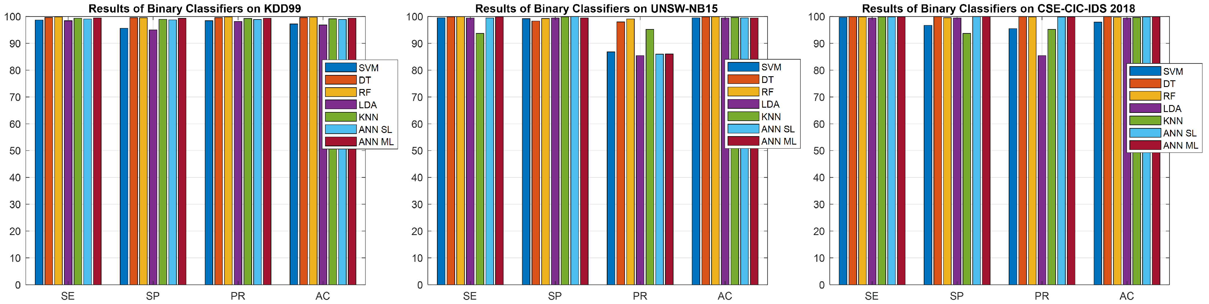
| KDD 99 | UNSW-NB15 | CSE-CIC-IDS 2018 | ||||||||||
|---|---|---|---|---|---|---|---|---|---|---|---|---|
| SE | SP | PR | AC | SE | SP | PR | AC | SE | SP | PR | AC | |
| SVM | 98.69% | 95.60% | 98.45% | 97.25% | 99.50% | 99.22% | 86.80% | 99.49% | 99.71% | 96.72% | 95.51% | 97.95% |
| DT | 99.65% | 99.60% | 99.60% | 99.63% | 99.93% | 98.30% | 98.0% | 99.88% | 99.99% | 99.99% | 99.99% | 99.99% |
| RF | 99.90% | 99.57% | 99.89% | 99.75% | 99.97% | 99.25% | 99.08% | 99.95% | 99.90% | 99.57% | 99.89% | 99.75% |
| LDA | 98.44% | 95.04% | 98.15% | 96.85% | 99.45% | 99.46% | 85.43% | 99.45% | 99.45% | 99.46% | 85.43% | 99.45% |
| KNN | 99.36% | 98.97% | 99.26% | 99.18% | 93.71% | 99.85% | 95.23% | 99.65% | 99.85% | 93.71% | 95.23% | 99.65% |
| ANN SL | 99.07% | 98.72% | 98.90% | 98.92% | 99.46% | 100% | 85.97% | 99.48% | 99.86% | 99.99% | 99.81% | 99.92% |
| ANN ML | 99.46% | 99.30% | 99.36% | 99.39% | 99.94% | 99.46% | 86.01% | 99.45% | 99.93% | 100% | 99.91% | 99.96% |
| UNSW-NB15 | CSE-CIC-IDS 2018 | |||||||
|---|---|---|---|---|---|---|---|---|
| M-SE | M-SP | M-PR | M-AC | M-SE | M-SP | M-PR | M-AC | |
| SVM | 75.52% | 93.88% | 77.44% | 75.52% | 86.67% | 98.52% | 90.17% | 86.68% |
| DT | 79.74% | 94.93% | 82.10% | 79.74% | 94.99% | 99.44% | 96.20% | 94.99% |
| RF | 80.20% | 95.05% | 83.08% | 80.20% | 94.17% | 99.35% | 95.08% | 94.20% |
| LDA | 71.34% | 92.83% | 73.07% | 71.34% | 85.36% | 98.37% | 86.80% | 85.34% |
| KNN | 69.03% | 92.26% | 69.80% | 69.04% | 90.21% | 98.92% | 90.43% | 90.20% |
| ANN ML | 79.85% | 94.97% | 82.20% | 79.90% | 89.62% | 98.84% | 91.31% | 89.60% |
| KDD 99 | UNSW-NB15 | CSE-CIC-IDS 2018 | |||
|---|---|---|---|---|---|
| Binary | Binary | Multiclass | Binary | Multiclass | |
| SVM | 24.08 ms | 26.70 ms | 29.72 ms | 44.40 ms | 383.51 ms |
| DT | 07.54 ms | 10.59 ms | 17.31 ms | 04.44 ms | 07.78 ms |
| RF | 77.82 ms | 85.67 ms | 105.82 ms | 80.30 ms | 136.84 ms |
| LDA | 10.48 ms | 20.62 ms | 33.23 ms | 07.38 ms | 11.30 ms |
| KNN | 453.12 ms | 2806 ms | 30,902 ms | 878 ms | 1354 ms |
| ANN SL | 20.74 ms | 31.67 ms | \ | 17.25 ms | \ |
| ANN ML | 40.56 ms | 68.78 ms | 75.39 ms | 35.20 ms | 54.73 ms |
| CSE-CIC-IDS 2018 | |
|---|---|
| Attack Type | Percent |
| Bot | 10% |
| DDoS attack HOIC | 10% |
| DDoS attack LOIC HTTP | 10% |
| DoS attack GoldenEye | 10% |
| DoS attack Hulk | 10% |
| DoS attack SlowHTTP Test | 10% |
| DoS attack Slowloris | 10% |
| FTP Brute Force | 10% |
| Infiltration | 10% |
| SSH Brute Force | 10% |
| Total | 100% |
| Dataset | “Best” ML Models | Dataset Management | Performance | |
|---|---|---|---|---|
| KDD99 (only binary) | RF, DT and KNN | DT and KNN perform better with preliminary feature transformation, reduction and scaling. RF require less preliminary dataset manipulation. | Comparable performance with very high accuracy (>99%) and very low FPR (<0.5%) | [23,38,41] |
| UNSW-NB15 (both binary and multiclass) | RF and ANN | RF require feature reduction. ANN perform also without preliminary manipulation. | Comparable performance with very high accuracy and very low FPR in binary classification. RF perform better for multiclass IDS with medium accuracy (<85%) and low FPR (<1%) | [30,31] |
| CSE-CIC-IDS 2018 (both binary and multiclass) | DT, RF and KNN | Required complete dataset manipulation Workflow. | Comparable performance with very high accuracy and very low FPR in binary classification. RF perform better for multiclass IDS with medium-high accuracy (<90%) and low FPR (<1%) | [19,41] |
Disclaimer/Publisher’s Note: The statements, opinions and data contained in all publications are solely those of the individual author(s) and contributor(s) and not of MDPI and/or the editor(s). MDPI and/or the editor(s) disclaim responsibility for any injury to people or property resulting from any ideas, methods, instructions or products referred to in the content. |
© 2023 by the authors. Licensee MDPI, Basel, Switzerland. This article is an open access article distributed under the terms and conditions of the Creative Commons Attribution (CC BY) license (https://creativecommons.org/licenses/by/4.0/).
Share and Cite
Dini, P.; Elhanashi, A.; Begni, A.; Saponara, S.; Zheng, Q.; Gasmi, K. Overview on Intrusion Detection Systems Design Exploiting Machine Learning for Networking Cybersecurity. Appl. Sci. 2023, 13, 7507. https://doi.org/10.3390/app13137507
Dini P, Elhanashi A, Begni A, Saponara S, Zheng Q, Gasmi K. Overview on Intrusion Detection Systems Design Exploiting Machine Learning for Networking Cybersecurity. Applied Sciences. 2023; 13(13):7507. https://doi.org/10.3390/app13137507
Chicago/Turabian StyleDini, Pierpaolo, Abdussalam Elhanashi, Andrea Begni, Sergio Saponara, Qinghe Zheng, and Kaouther Gasmi. 2023. "Overview on Intrusion Detection Systems Design Exploiting Machine Learning for Networking Cybersecurity" Applied Sciences 13, no. 13: 7507. https://doi.org/10.3390/app13137507
APA StyleDini, P., Elhanashi, A., Begni, A., Saponara, S., Zheng, Q., & Gasmi, K. (2023). Overview on Intrusion Detection Systems Design Exploiting Machine Learning for Networking Cybersecurity. Applied Sciences, 13(13), 7507. https://doi.org/10.3390/app13137507