Experimental and Numerical Study on the Slug Characteristics and Flow-Induced Vibration of a Subsea Rigid M-Shaped Jumper

Abstract

The subsea jumper has become an essential part of subsea production systems as a gas–liquid mixing pipeline connecting the pipeline end manifold (PLEM) to the Christmas tree. During oil and gas transportation, as a common flow pattern, the alternating flow characteristics of the slug flow easily cause pipeline vibration, resulting in pipeline instability or fatigue damage. The present study investigates experimentally and numerically the slug flow characteristics in the subsea M-shaped jumper and its induced vibrations of the jumper. The flow pattern evolution and slug characteristics of the inner slug flow under different gas–liquid velocities are obtained: the slug frequency and slug velocity, as well as the pressure fluctuation and vibration characteristics caused by the slug flow. The results show that the pressure fluctuations in the front and rear parts of the M-type jumper are obviously different. With the increase in the air–water mixing, the two characteristics, the slug frequency, and the slug velocity also increase. The gas velocity has a greater influence on the slug frequency than the liquid velocity. The slug length decreases as the slug frequency increases. Furthermore, numerical simulations under various experimental conditions are carried out. The results show that the simulation results of the pressure data, the slug characteristics, and the induced vibration amplitude are in good agreement with the experimental data.

1. Introduction

In recent years, the safety of submarine oil and gas transportation pipelines has become a key priority due to the gradual expansion of oil and gas exploitation in the deep sea, and pipeline vibration is the primary source of fatigue damage. According to a study by the UK Health and Safety Executive (HSE), 21% of pipeline damage in the UK’s offshore industry in the North Sea is due to vibration-induced pipeline fatigue failure [1]. Subsea jumpers play a vital role in oil and gas production systems, connecting elements of subsea structures, such as pipe manifolds, Christmas trees, risers, and pipeline terminals. As shown in Figure 1, compared to ordinary subsea pipelines, the subsea jumper has a unique multi-bending structure and long overhanging sections, which leads to a greater impact on the pipeline in the process of oil and gas transportation due to a slug flow formed inside the pipeline.

Slug flow is a transient flow. In the classification method of multiphase flow patterns, based on the flow medium’s continuity, the state of the medium is diffuse, intermittent, and continuous. Based on this concept, slug flow can be defined as an intermittent flow state. Since the subsea jumper has several elbows and straight pipes, some of the methods and conclusions obtained by studying the flow inside the elbows and straight pipes and their vibration patterns can still be applied to the subsea jumper. For the characteristics of the internal slug flow of straight pipes and the vibration induced by the slug flow of straight pipes, many researchers have carried out investigations by theoretical analysis, experiments, and numerical simulations. To determine the relationships among two-phase flow parameters, including the slug length, slip ratio, void ratio, and pipe vibration, Bamidele et al. [3] conducted an experimental investigation of the slug flow-induced vibration characteristics of a horizontal pipe with a throttle aperture. Mohmmed [4] used unidirectional fluid–structure interaction simulations and experimental methods to analyze how horizontal pipes and slug flow interacted. The simulation and experimental results were in good agreement. Cabrera-Miranda J.M. [5] studied the nonlinear planar vibration of risers excited by a two-phase flow using a model of a steady-state slug flow and provided guidance for the design of a riser considering the slug frequency and slug length. Al-Hashimy et al. [6] conducted an experimental investigation of slug flow in a horizontal pipe and found that the vibration displacement of the pipe increased with the increasing liquid velocity at a specific air velocity. Zhu et al. [7] conducted an experimental study on a free-hanging flexible riser with three slug flow patterns at specific flow rates. Dinaryanto et al. [8] conducted an experimental investigation on a gas–liquid two-phase slug flow inside a horizontal pipe with an inner diameter of 26 mm. The mechanism of slug formation and the pressure fluctuations were investigated by visual observation. It was found that the slug was caused by Kelvin–Helmholtz instability. In addition, the slugs were formed at high gas velocities by merged multiple wave-like flows. Moh Yaseen et al. [9] used numerical simulations to explore the Marangoni boundary condition to explore the MHD nonlinear convective nanofluid and hybrid nanofluid flow and heat transport over a vertical flat plate with the Marangoni boundary condition. Cao et al. [10] used a combination of experimental and numerical simulations to study the slug flow characteristics in horizontal bends and summarized a law governing the fluid distribution, void fraction, pressure, and liquid film velocity in the pipe under slug flow conditions. Moh Yaseen et al. [11] used numerical simulations to deal with a bioconvective 2D THNF flow containing a microbial suspension toward three different geometries (a flat plate, a wedge, and a cone) with the suction/injection effect. Shi et al. [12] and Zahedi et al. [13] both researched slug flow patterns in curved pipes with different radii of the curvature and used dynamic slug flow models to simulate completions and throttling under site conditions. Wang et al. [14] simulated a slug flow in a 90-degree bend by fluid–structure interaction and obtained the flow pattern distribution and structural response in the pipe. A higher superficial gas velocity of the slug flows had a more severe periodic effect on the pipeline. Liu et al. [15] carried out an experimental study using a 90-degree bend with an inner diameter of 52.5 mm to investigate the pulsation forces induced by internal two-phase flow over the bend and showed that the dominant frequency of the pulsation forces peaked in the slug flow region and increased monotonically with the superficial gas velocity. Bamidele et al. [16] analyzed the vibrations caused by bubble flow, slug flow, wave flow, and annular flow in U-shaped tubes and proposed a mathematical model to predict the impact force of the U-tubes.

The geometry of the jumper is more complex than that of the elbow, which consists of multiple bends and a long overhanging section. Slug flow exhibits a more complex behavior as it flows through the jumper, where successive elbows cause the transition of the slug characteristics. To the authors’ knowledge, the investigations on the two-phase flow in the subsea jumper have mostly been conducted by numerical simulations. Chica et al. [17] analyzed the vibration induced by the slug flow using a combination of CFD and computational structural dynamics (CSD) simulations in a subsea rigid jumper and obtained the frequency of the slug flow by tracking the slug in the pipe using the VOF model. Van der Heijden et al. [18] used a three-beam model to analyze the vibration displacement response of the jumper at different slug velocities and found that the fatigue damage degree of the jumper correlated with the flow rate of the slug. Voronkov et al. [19] analyzed the flow-induced vibrations in a subsea jumper using bi-directional fluid–structure interaction (FSI) simulations, evaluated the impact on the fatigue life of the jumper, and finally concluded that the FSI can be captured using a one-way fluid–structure coupling. Jia et al. [20] set the length and frequency of the slug by numerical simulation to study the interaction characteristics of the two gas–liquid phases in the jumper interior. Nair et al. [21] carried out numerical simulations on the slug in a multi-plane jumper and used a finite element model (FEM) to analyze the fatigue damage of the jumper. Pontaza et al. [22] conducted a three-dimensional numerical simulation of the vibration process caused by the slug flow in the jumper, estimated the structural response of the jumper, including the fatigue life, and found that the main frequency of the pipe vibration was related to modes 1–4, and the stress is highest when the gas volume fraction was 55%. Later, Pontaza et al. [23] evaluated the vibration fatigue caused by a flow of water injection across a pipe using a thermoplastic composite pipe (TCP) and used a three-layer screening method to evaluate the degree of vibration fatigue damage expected in this TCP jumper application. Kim et al. [24] evaluated the dynamic response of a jumper through a one-way fluid–structure interaction method and discussed the potential resonance through modal analysis. Le Prin et al. [25] analyzed the flow-induced vibrations caused by the slug flow in a jumper through numerical simulations and compared the results with current examples in subsea pipeline design to ensure the accuracy of the simulations.

In summary, the current research on slug flow in the literature has mainly focused on simple pipelines, such as horizontal straight pipes and 90-degree bend pipes, and the slug flow in a subsea jumper has rarely been involved. Meanwhile, for subsea jumpers with complex geometric structures, a few studies have been carried out using numerical simulations, but the research conditions have been singular, and the corresponding data support and experimental verification are lacking. Therefore, in the present study, to obtain a good understanding of the development of the slug flow inside subsea jumpers, a combination of a numerical simulation and an experimental study was used to investigate the slug characteristics, such as the slug length, slug frequency, and slug velocity, inside a subsea jumper and the slug flow-induced vibration characteristics of the jumper. The corresponding experimental data can verify the employed numerical model, and they also provide a certain reference for subsea jumpers’ design, safe operation, and vibration control. In the present study, an experimental circuit was established. A visualization of the two-phase flow was conducted using a high-speed camera to analyze the flow characteristics and slug characteristics of the internal gas–liquid slug flow. Pressure sensors and accelerometers recorded the pressure and vibration data to investigate the relationship between the slug characteristics and the pressure and the induced vibration. The VOF model and the unidirectional fluid–structure coupling method were used in the numerical simulations to investigate the interaction between the slug flow and the jumper at various mixing gas–liquid velocities. The organization of the article’s structure is as follows: The multiphase flow experimental device used in this work is briefly introduced in Section 2. The multiphase flow model for the numerical simulations and the mesh convergence studies are introduced in Section 3. The analysis of the slug characteristics and the induced flow vibration characteristics under the experimental conditions, the analysis of the numerical simulation results, and a comparison with the experimental results are given in Section 4. Finally, the conclusion is provided in Section 5.

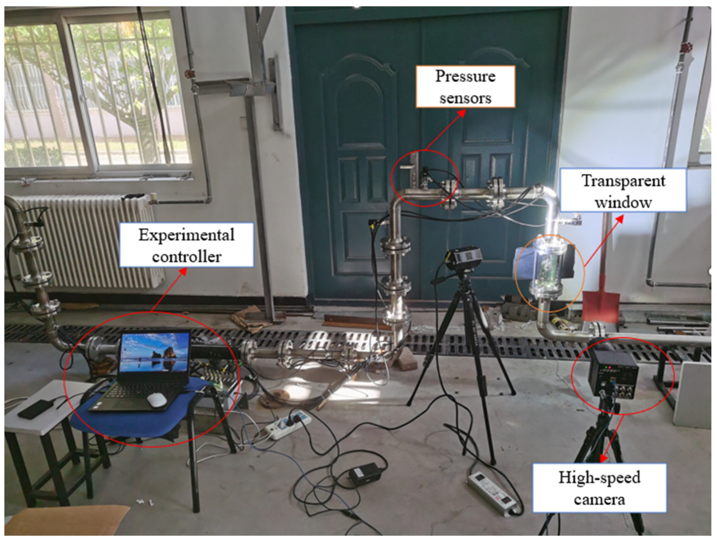
2. Experimental Work

As illustrated in Figure 2, an experimental investigation into the slug characteristics of a subsea M-shaped jumper’s inner slug flow and the flow-induced vibration was conducted with the support of Dalian Maritime University’s multiphase flow experimental platform. The experimental circuit is mainly composed of one three-phase separator, two pumps (oil pump and water pump), a flow-regulating valve, air compressors, an air bottle, a freeze dryer, mixing pipelines, and various experimental circuits (including jumpers). Two air compressors with a combined rated volume flow rate of 1020 m³/h and a maximum exhaust pressure of 20 bar are available in the lab to deliver compressed air for the experimental gas phase. The air compressor compresses the air and then enters the air bottle with a volume of 2 m³ and a 3 MPa maximum operating pressure. The laboratory is equipped with two vertical multistage centrifugal pumps to provide water for the liquid phase in the experiment, for one single pump with a maximum flow rate of 100 m³/h. Proportional–integral–derivative (PID) control was utilized during the investigation to precisely control the gas flow-regulating valve and the pump variable frequency. Through the regulation of the ball valve opening after air and water have been combined in the gas–liquid mixing part, the gas–liquid flows into the experimental pipelines for experimental research, flows out from the outlet of the experimental section, and finally, the mixture enters the three-phase separator through the pipeline. After passing through the three-phase separator, the two vertical centrifugal pumps are used to pump the bottom water into the experimental pipe to create a circulating flow, and the separated air enters the atmosphere or is used to maintain a specific back-pressure.

The jumper consists of two ascending portions, three horizontal portions, and two descending portions, as depicted in Figure 3. The gas–liquid mixture flow in the jumper passes through six elbows, not including the inlet and outlet connection pipelines. The jumper parts of S1–S7 are flanged connections and are swapped out for transparent windows of the same size to visualize the slug flow inside the jumper. The transparent window is made of Plexiglas material to ensure that it is transparent to meet observational standards and can sustain a fluid pressure of up to 2 MPa. Additionally, reinforced support is used to guarantee the security of the piping connections and transparent windows.

Table 1. The subsea jumper model’s parameters.

Parameter	Values	Dimension
Total length	3.6	m
Inner diameter	0.048	m
Wall thickness	0.004	m
Curvature radius	1.5 D
Transparent section length	0.23	m
Density	7850	kg/m3
Poisson’s ratio	0.3
Young’s modulus	2.06 × 105	MPa

displays the jumper’s physical properties. The experimental jumper has a diameter of 52 mm, an inner diameter of 48 mm, and a wall thickness of 4 mm.

The physical properties of the two experiment-related media are listed in

Table 2. The physical properties of the fluids.

${\mathbf{\rho }}_{\mathbf{g}}$	${\mathbf{\rho }}_1$	${\mathbf{\mu }}_{\mathbf{g}}$	${\mathbf{\mu }}_1$	Surface Tension Coefficient
(kg/m3)	(kg/m3)	(kg/m·s)	(kg/m·s)	(N/m)
1.29	998.2	1.8 × 10−5	1.0 × 10−3	0.072

. Given their low flow rates and flow pressures, the compressibility of the fluids was not considered.

A high-speed camera was positioned to capture the slug characteristics of the slug flow in the jumper. The actual piping diagram of the subsea jumper is depicted in Figure 4. The high-speed camera required high accuracy, and the Mini UX100 system developed by Japan’s FASTCAM company was chosen. Its capture speed (full frame) was up to 4000 fps. The high-speed camera had to shoot when the light intake was low. To ensure there was enough light intensity for the high-speed camera to catch the rigid jumper inner gas–liquid flow, an LED fill light was installed on the side of the pipeline.

Eight pressure sensors were inserted into the elbow portion of the jumper, as can be seen in Figure 4, to track pressure changes in various locations. The S-20.0-2.5 series pressure sensor developed by Germany’s Wika company was adopted. It has an accuracy of 0.1% and a working range from 0 to 2.5 MPa. The pressure sensor was threaded to the rigid jumper via NPT. It emitted a voltage signal of 0–5 V, and the sampling rate was set to 1000 Hz. An NI-USB-6210 series acquisition card developed by America was used, and the upper computer was equipped with an NI data acquisition system for data acquisition, storage, and export.

As Figure 5 shows the jumper section slug flow-induced vibration experimental system. To prevent the flanges and transparent windows on the jumper from affecting the vibration characteristics of the pipe, the same-size rigid jumper was selected for the vibration experiments, and fixed constraints were set on both ends. The LC0103 has a built-in IC piezoelectric accelerometer to measure vibration, and the accelerometer was installed in different positions to obtain the vibration characteristics of the pipeline. The sensor sensitivity was 50 mV/g, and the frequency range was 0.35–10,000 Hz. The LC3101 data-collecting device developed by SANYO was used to enable multi-channel sampling, and the obtained data were then transmitted via a USB interface to the host computer for monitoring in real time as well as saving.

3. Numerical Models

Computational fluid dynamics (CFD) techniques have been extensively applied to investigate the evolution characteristics of gas–liquid two-phase flow in pipelines. The volume of fluid (VOF) model is a Eulerian–Eulerian approach to capture crucial interfacial properties. The gas–liquid interface in slug flow was tracked using the VOF model.

3.1. The VOF Model

Hirt and Nichols [26] were the ones who first put forth the VOF model to solve the flow of two or more immiscible fluids. The tracking of the gas–liquid interface in this model is carried out by solving the continuity equation. The gas phase and the liquid phase share a momentum equation [27]. The governing equations of the VOF model are listed here:

The continuity equation [28]:

$$\frac{\partial \rho }{\partial t}+\nabla ·(\rho \mathsf{u})=0$$

(1)

where $\rho$ and $t$ are the density of the fluids and the time, respectively, and $\mathsf{u}$ stands for the velocity vector.

The momentum equation [26]:

$$\frac{\partial (\rho \mathsf{u})}{\partial t}+\nabla ·\left(\rho \mathsf{u}\mathsf{u}\right)=-\nabla P+\nabla \mu \left(\nabla \mathsf{u}+\nabla {\mathsf{u}}^T\right)+\mathit{F}$$

(2)

where $\mu$, $P$ and $\mathit{F}$ are the viscosity of the fluids, the pressure, and the surface tension force of the fluids, respectively.

The continuity equation for one phase (which generally refers to the liquid phase) can be solved to determine the location of the interface between the gas phase and the liquid phase [14]. The following equation is displayed:

$$\frac{\partial {\alpha }_i}{\partial t}+\mathsf{u}·\nabla {\alpha }_i=0$$

(3)

The continuous surface force (CSF) model is used to obtain the surface tension between the gas and liquid. The momentum equation of Equation (2) includes the surface tension as a source term:

$$\mathit{F}={\sigma }_{ij}\left[\frac{\rho k_i\nabla {\alpha }_i}{\raisebox{1ex}{$\left({\rho }_i+{\rho }_j\right)$}\!\left/ \!\raisebox{-1ex}{$2$}\right.}\right]$$

(4)

where $\sigma$ represents the surface tension coefficient, and $k_i$ represents the surface curvature.

3.2. Turbulence Model

In the present study, the realizable turbulence model was used to resolve the complicated turbulence of the two-phase flow inside the jumper [29]. The governing equations of turbulent kinetic energy $k$ and the turbulent energy dissipation rate $\epsilon$ are given below:

$$\frac{\partial }{\partial t}\left(\rho k\right)+\frac{\partial }{\partial x_j}\left(\rho k{u}_j\right)=\frac{\partial }{\partial x_j}\left[\left(\mu +\frac{{\mu }_t}{{\sigma }_k}\right)\frac{\partial k}{\partial x_j}\right]+G_k+G_b-\rho \epsilon -Y_M+S_k$$

(5)

$$\begin{array}{l}\frac{\partial }{\partial t}\left(\rho \epsilon \right)+\frac{\partial }{\partial x_j}\left(\rho \epsilon u_j\right)=\frac{\partial }{\partial x_j}\left[\frac{\partial \epsilon }{\partial x_j}\left(\mu +\frac{{\mu }_t}{{\sigma }_k}\right)\right]+\\ \rho C_{1}S\epsilon -\rho C_2\frac{{\epsilon }^2}{k+\sqrt{\nu \epsilon }}+C_1{}_{\omega }\frac{\epsilon }{k}{C}_{3\epsilon }{G}_b+S_{\epsilon }\end{array}$$

(6)

where $G_k$ indicates the kinetic energy of turbulence generation. $Y_M$ represents the dissipation rate’s overall contribution from changing dilatation in compressible turbulence [30]. $G_b$ denotes the buoyancy-induced turbulence kinetic energy. The constants of the turbulent model are given below:

$$C_{1\omega }=1.44,{\sigma }_k=1.0,C_2=1.9,{\sigma }_{\epsilon }=1.2$$

3.3. FSI Model

Based on the principle of unidirectional coupling, the FSI coupling between the flow of the fluids and the transient structure solver was established on the ANSYS Workbench platform. The solid transient structure model received the pressure output from Fluent, which was then applied to the pipe wall as an excitation load. The transient pressure variations induced by the two-phase flow field caused the experimental jumper to display specific structural dynamic responses. The equations of motion based on Newton’s second law are given as:

$$\mathsf{M}\ddot{\mathsf{u}}\left(\mathsf{t}\right)+\mathsf{C}\dot{\mathsf{u}}\left(\mathsf{t}\right)+\mathsf{K}\mathrm{u}\left(\mathrm{t}\right)=\mathsf{f}\left(\mathsf{t}\right)$$

(7)

where $\mathsf{M}$ represents the matrix of the structural mass, $\mathsf{C}$ stands for the damping, and $\mathsf{K}$ is the donated stiffness matrix. $\ddot{\mathsf{u}}\left(\mathsf{t}\right)$ is the acceleration vector of the jumper, and $\dot{\mathsf{u}}\left(\mathsf{t}\right)$ represents the velocity vector of the jumper. $\mathrm{u}\left(\mathrm{t}\right)$ is the displacement vector of the jumper. $\mathsf{f}\left(\mathsf{t}\right)$ represents the vector of the load from the fluid domain [31].

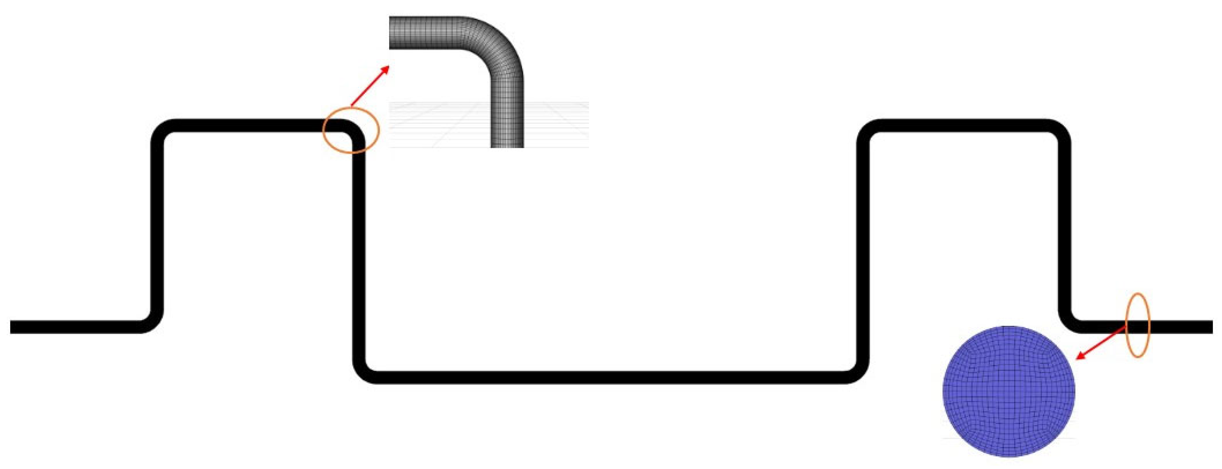
3.4. Boundary Conditions and Mesh Convergence Studies

In this numerical simulation, air and water were utilized as the first and second phases, respectively. The numerical model described above was solved using ANSYS Fluent software developed by America, and the surface tension coefficient between the two media remained constant at 0.072 N/m. The turbulence effect was resolved via the model. A standard wall function was set to solve the boundary layer of the experimental jumper. The velocity input and pressure outlet were specified, and the wall was given a non-slip wall boundary condition.

The momentum equation was solved using the QUICK format, the pressure equation was solved using the PRESTO scheme, and the relaxation factor was set at 0.7 for the pressure and 0.3 for the momentum. To ensure the stability of the simulations, the CFL (Courant–Friedrichs–Lewy) number was kept below 1 during the simulations. As described in Figure 6, structured meshes generated using the ICEM tool were used to discretize the computational domain of the fluid.

A mesh convergence study was performed to determine the optimal number of grids. Generally, a larger number of grids leads to more accurate simulation results while significantly increasing the computing cost. An appropriate number of meshes should be selected to balance the computational accuracy and resources. Three different meshes with grids numbers of M₁: 663,022, M₂: 883,268, and M₃: 1,109,088 were used to carry out the simulations under the working condition of a mixing velocity of 2 m/s and a gas content of 50% as the representative case. The maximum pressure was monitored at P1, and the time-averaged value of the pressure difference between P1 and P2 was used to evaluate the grid resolutions. The results using the three meshes are compared in Figure 7. The relative discrepancy among the results of the three grids was within 5%. Considering the computational accuracy, cost, and efficiency, the mesh with a total grid number of 883,268 was chosen for the simulations.

4. Results and Discussion

In the experiment, it should be noted that when collecting the data for each experimental condition, it was necessary to ensure that the data collection time for each condition was sufficiently long to facilitate statistics to ensure that the time-averaged pressure and the root mean square value of the vibration amplitude did not change with the increasing time. The pressure fluctuation at P1 was measured twice at a gas–liquid mixing speed of 1 m/s with a gas content of 50%. By using fast Fourier transform, the measured data were transformed from the time domain to the frequency domain, and the results obtained twice were compared. The distribution patterns of the two power spectral densities (PSDs) were similar, and their dominant frequencies and amplitudes were generally the same, as shown in Figure 8, demonstrating the consistency and independence of the experimental measurements.

Before starting the studies involving two-phase flow, modal analysis was performed for the jumper structure using the hammering method to determine the natural frequencies of the jumper under two states—the empty jumper and the jumper filled with water. The hammering method was conducted by utilizing several points of excitation and three-point responses. Fast Fourier transform was performed on the acceleration signal acquired at two points on the jumper to obtain the first six orders of the natural structural frequency of the rigid M-shaped jumper, as displayed in

Table 3. The first six natural frequencies with empty and water-filled jumpers.

Mode	${\mathit{f}}_{\mathit{i}\mathit{e}}$ (Hz)	${\mathit{f}}_{\mathit{i}\mathit{f}}$ (Hz)
1	7.44	5.89
2	10.39	7.56
3	12.58	9.42
4	16.68	13.67
5	16.97	14.78
6	19.11	18.23

. It can be seen that with the jumpers filled with water, the natural frequency of each order was reduced.

To characterize the slug flow, all the conditions used in the experiment are represented in the flow diagram shown in Figure 9. All of the experimental conditions of the present investigation belonged to the slug flow condition.

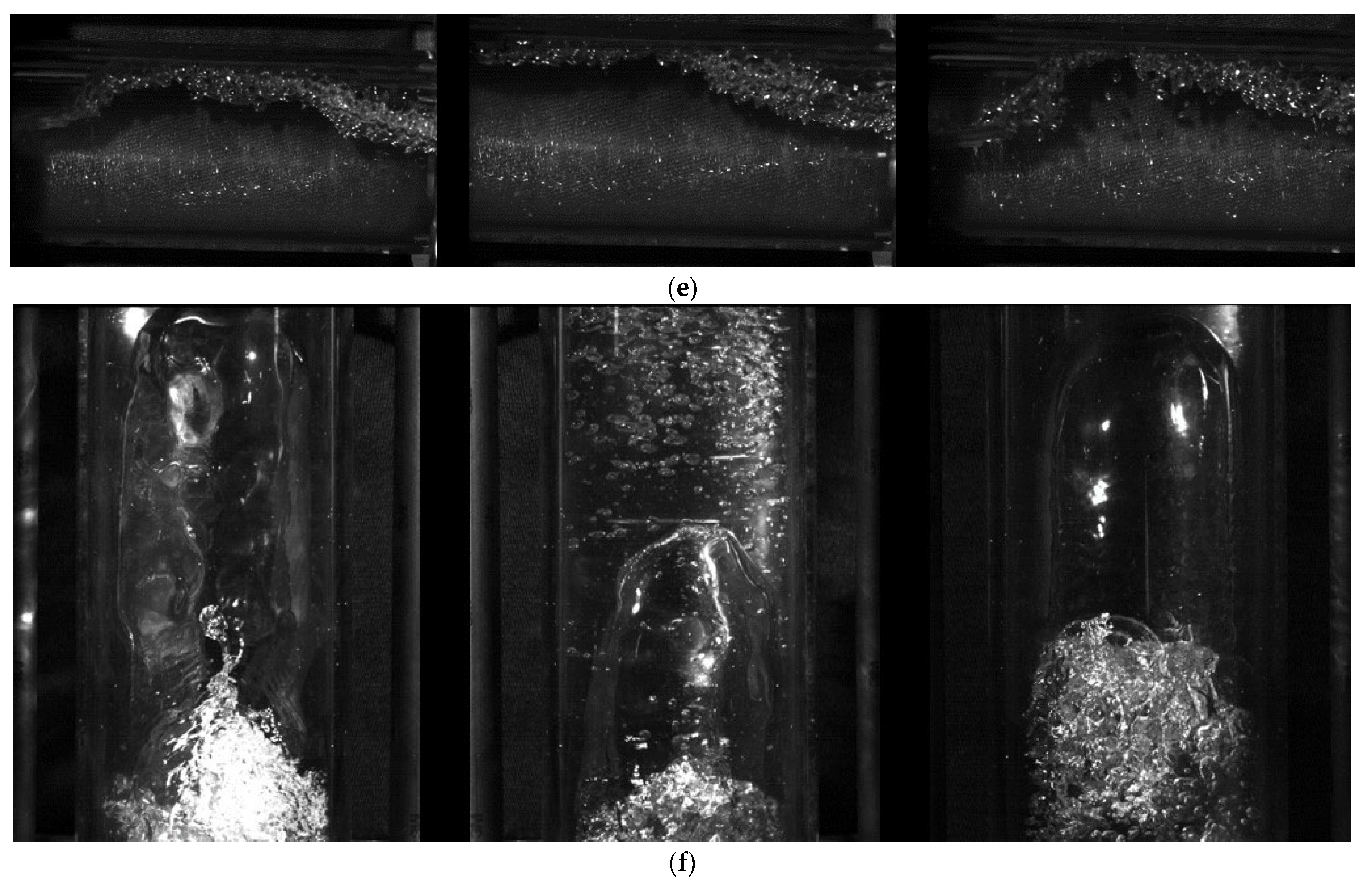
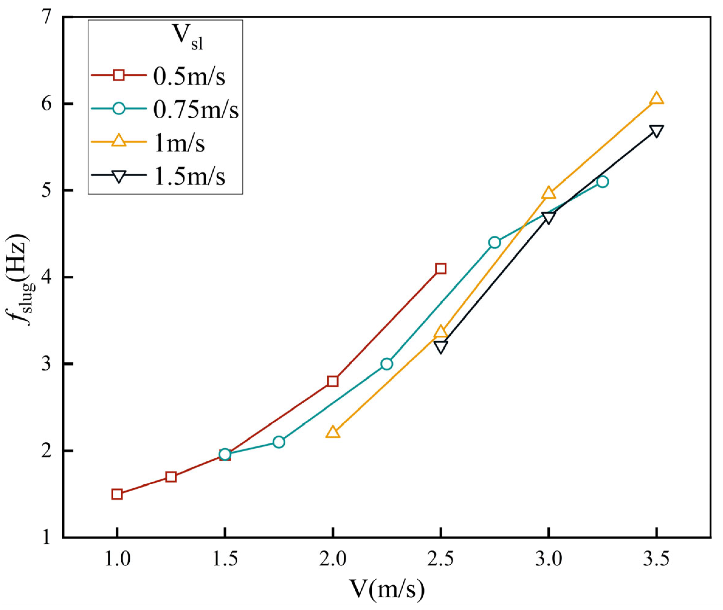
4.1. Visualization of the Slug Flow

Before collecting the pressure and vibration data, a visualization of the slug flow within the subsea jumper was performed to qualitatively understand the evolution of the flow patterns of the slug flow through the jumper and the associated flow characteristics. Images of a typical slug flow are illustrated in Figure 10. As shown in Figure 10, the flow was dominated by a slug flow in the rising section (S1 section) of the jumper. As shown in Figure 10a, a bullet-shaped bubble characterizing a Taylor bubble appeared in the jumper, with a spherical head and a flattened tail. As can be seen in Figure 10b, when the liquid continued to flow upward and reached the horizontal section S2 after the elbow, the liquid phase accumulated at the elbow and occupied a large part of the volume due to the steering effect of the elbow. The subsequent bubbles continued to be pushed upward, causing the instability of the gas–liquid flow. An alternating gas–liquid flow was observed at the S2 pipe section, which is an obvious characteristic of a segment plug flow between the states of a wave flow and a slug flow, but a small amount of gas was still observed at the top of the liquid slug. The gas–liquid continued to flow under the effect of gravity when it reached S3 because the S3 pipe section was located in the descending pipe section, as shown in Figure 10c. In this section, the flow pattern changed to the churn flow, and the pipe was filled with small-scale broken bubbles in irregular shapes scattered throughout the liquid phase. The gas–liquid continued to be pushed forward, and when it reached the longer overhanging horizontal section S4 after the elbow, the gas–liquid flow gradually stabilized and showed a stratified flow pattern, as shown in Figure 10d. After an elbow, the flow entered the S5 rising portion after the gas and liquid flow passed through the overhanging area, and the flow pattern redisplayed a slug flow pattern, as shown in Figure 10e. However, different from the flow pattern in S1, the length of the Taylor bubble was smaller than that through S1. The flow pattern in section S6 of the pipeline was similar to that in section S2. However, since the rising section of S5 was longer than the rising section of S1, less liquid was accumulated at the elbow, as shown in Figure 10f, compared to Figure 10b, and the flow pattern resembled a wave flow. In the falling section of S7, the gas–liquid flow rate decreased due to energy loss, as can be seen in Figure 10g. A liquid film formed on both sides of the jumper wall and the flow pattern was an annular flow.

4.2. Pressure Fluctuations and Vibration Characteristics Caused by the Slug Flow

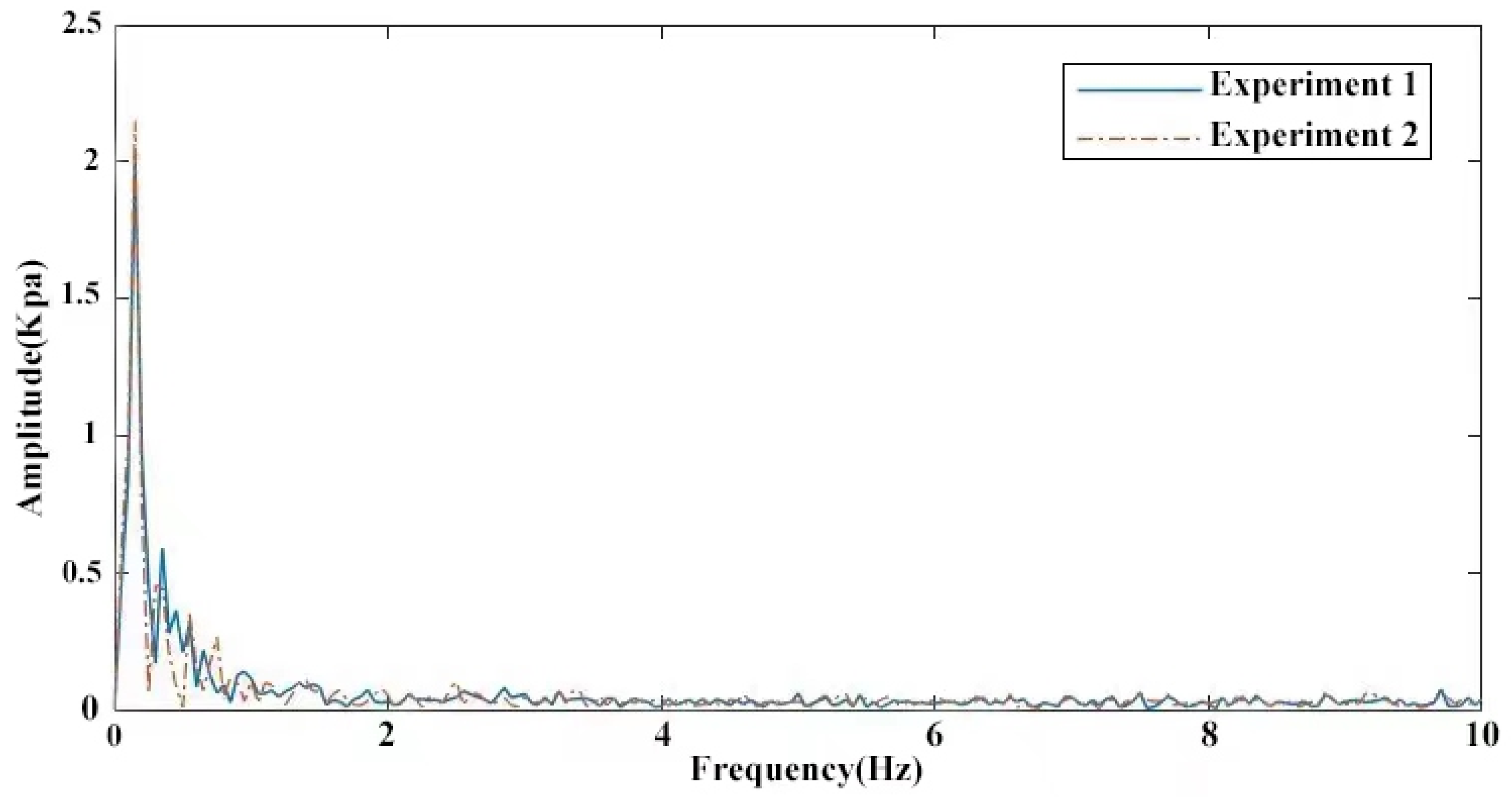
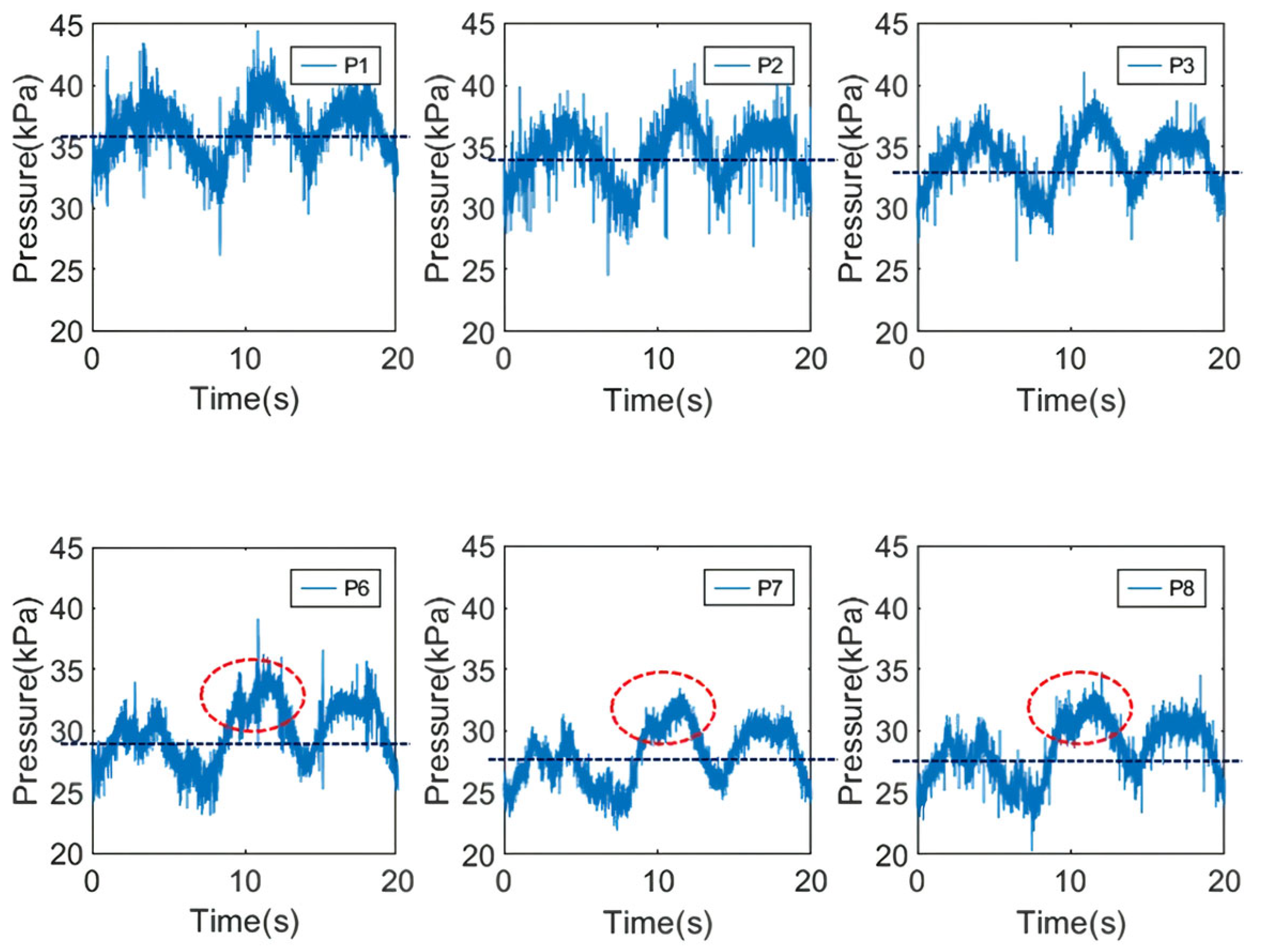
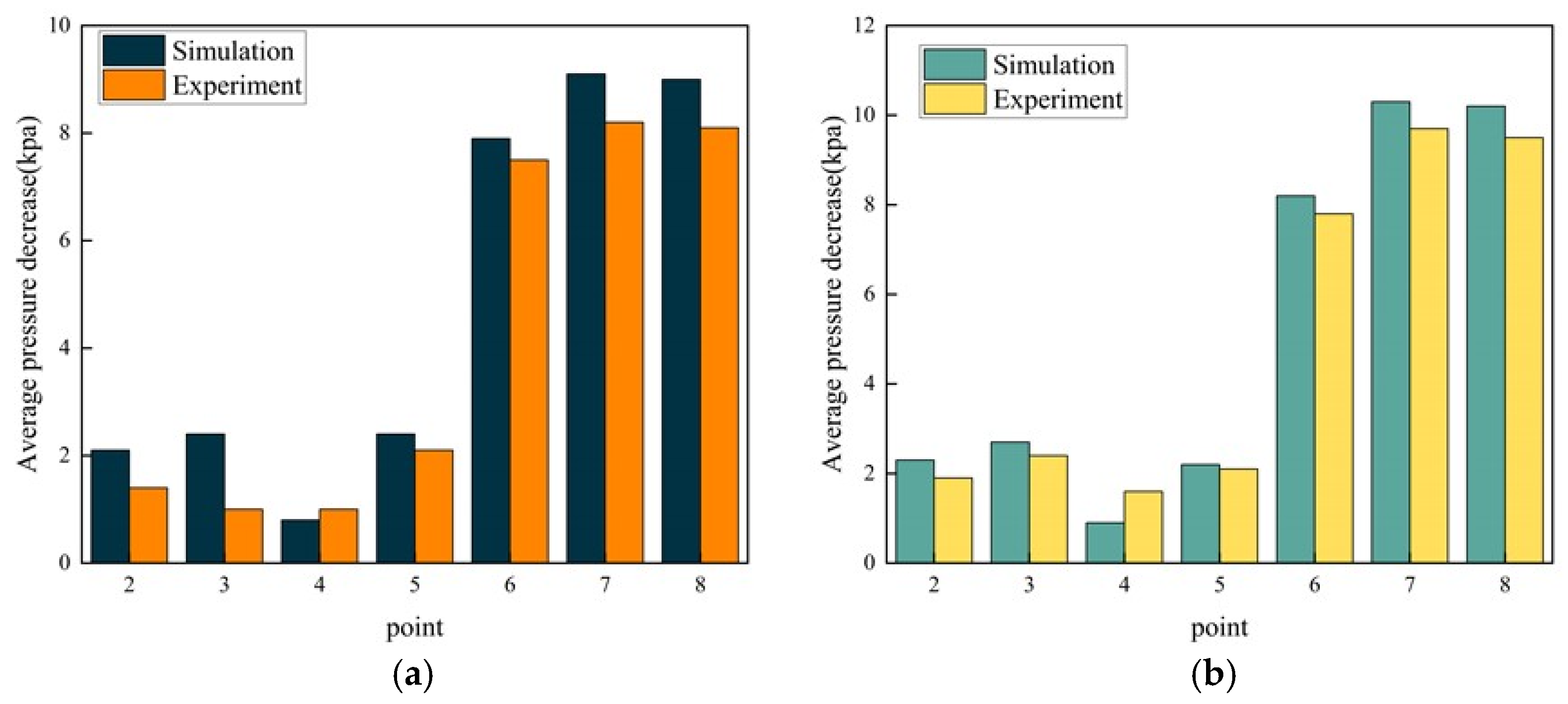
4.2.1. Pressure Fluctuations and Comparisons

The internal pressure fluctuation across the jumper caused by the slug flow was analyzed by selecting a typical slug flow condition of V_sl = 0.5 m/s and V_sg = 0.5 m/s. The temporal evolutions of the pressure measured by the pressure sensors P1, P2, P3, P6, P7, and P8 in the experiment are shown in Figure 11. P1, P2, and P3 represent the pressure fluctuations across the three sections of jumper S1, S2, and S3. The time-averaged flow pressure of the fluid gradually decreased after the gas–liquid two-phase entered from the inlet and flowed through several elbows as a result of the pressure loss caused by the friction between the gas–liquid flow and the pipe wall, as well as by the local pressure loss through the elbow.

The figure shows strong spikes in the time histories of the pressure at P1, P2, and P3, indicating a clear phase separation of the two-phase flow. The gas phase in section S1 merged in the form of a large gas bubble. When it flowed through the pressure measurement point, a gradual pressure drop was detected, followed by a gradual rise in the pressure when the liquid plug passed through, showing an obvious periodic change. At P6-P8, a bimodal structure with obvious pressure fluctuations was observed (denoted by the red dashed circles in Figure 11) because there was more gas–liquid mixture in this section of flow. As in section S6, the flow pattern was similar to the wavy flow of the segment plugs, and the flow in section S5 led to less gas phase buildup at the elbow, causing a relatively large disturbance to the liquid phase. Thus, inside the red dashed circles in Figure 11, a secondary fluctuation in the pressure extremum was observed in a short period of time.

The PSDs of the pressure in the frequency domain were obtained by using fast Fourier transformation for the pressure fluctuations, as illustrated in Figure 12. It can be seen that the dominant frequency of the pressure variation was 0.15 Hz. The overall dominant pressure fluctuation frequency was low. The alternating gas–liquid flow mainly caused the pressure fluctuation. The M-shaped jumper used in the experiment was a symmetrical structure; the first and second halves were composed of a rising section, a horizontal section, and a falling section. From the pressure time domain fluctuations, it can be seen that the first half of the pressure measurement points (P1, P2, P3) and the second half of the pressure measurement points (P6, P7, P8) show generally similar spectra distributions, which was due to the similarity of the flow trend caused by the structural similarity of the first and second sections. However, the second half of the section was influenced by the flow of the first half and exhibited different pressure variation characteristics from the first section. There was an obvious second harmonic frequency at 0.3 Hz in addition to the primary frequencies at P6, P7, and P8.

In the one-way fluid–structure coupling analysis, the pressure measured in Fluent needed to be transferred to the structural response model. Therefore, the pressure data obtained from the numerical simulations using Fluent needed to be compared with the pressure data obtained from the experiments to validate the numerical model and to ensure the accuracy of the structural calculation model. A numerical simulation was carried out for the slug flow conditions of V_sl = 0.5 m/s, V_sg = 0.5 m/s and V_sl = 1 m/s, V_sg = 1 m/s, and the data of the two cases were compared and analyzed. Eight pressure-monitoring points were set at the same positions in the fluid domain as the eight pressure sensors on the experimental pipeline, and the pressure fluctuations within the flow field were monitored during the simulations. The pressure data at the initial time were unstable and transient. Therefore, the last 5 s of the simulated time data was used for comparative analysis when the pressure data at each monitoring point became stable. In Figure 13, a comparison of the time-averaged pressure drop between the numerical simulation data and experimental data at each point is shown. The results show that the pressure data collected during the simulation match well with the experimental data. The relative discrepancy between the simulations and the experiments is within 15%. A similar distribution among the detection points between the simulations and experiments can be observed, indicating the feasibility of the employed numerical model.

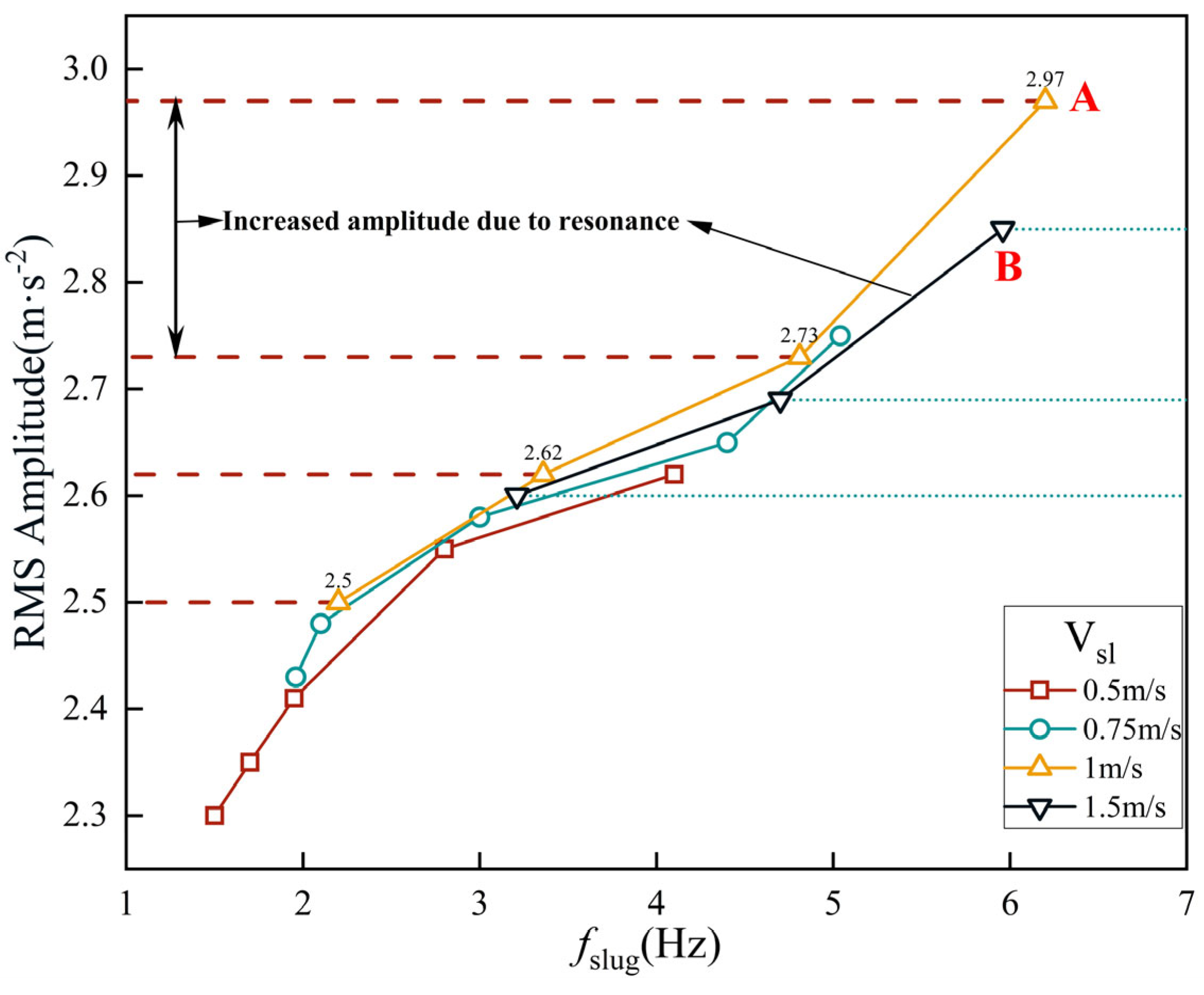
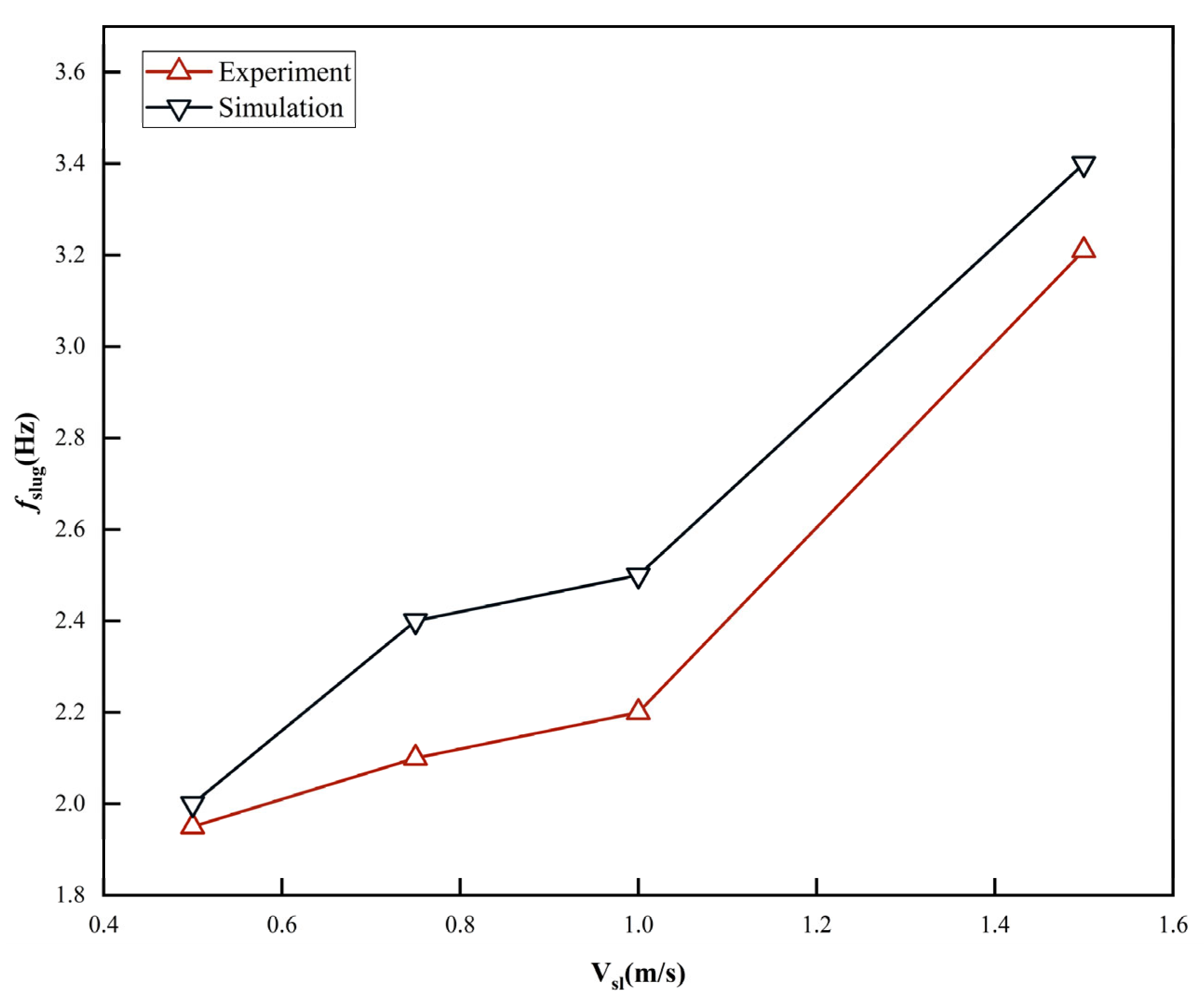
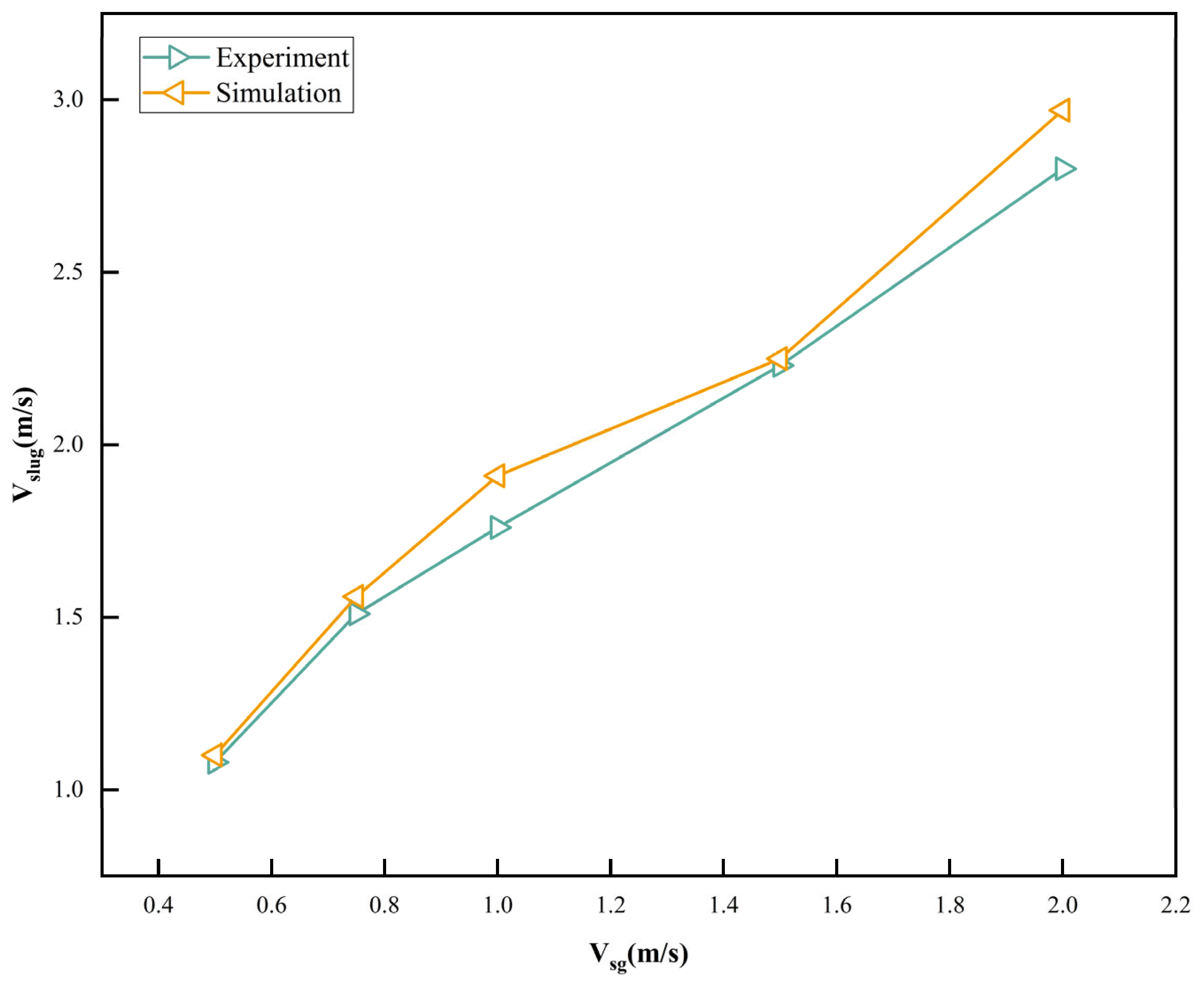
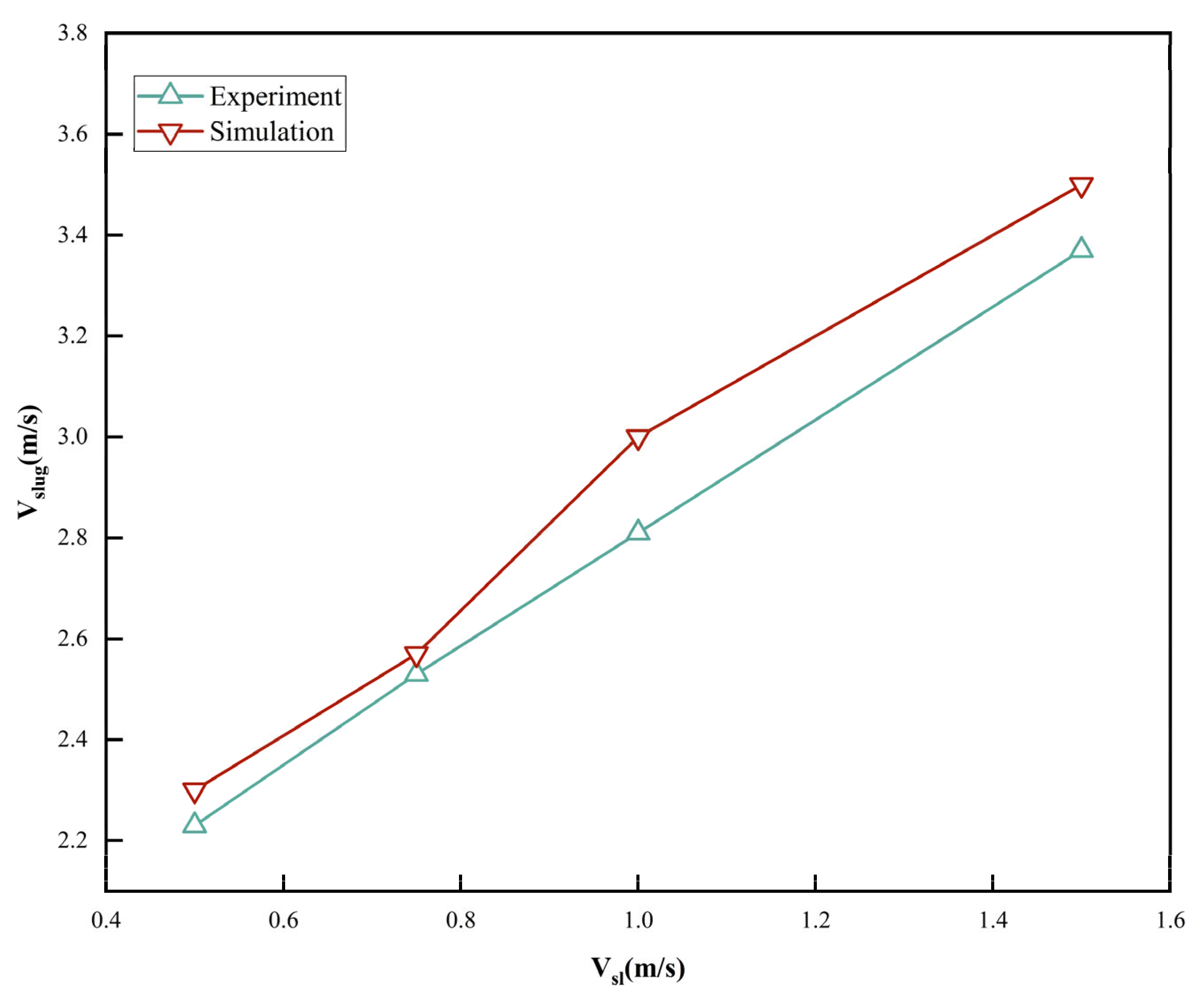
4.2.2. Effect on Vibration of Slug Flow Characteristics and Comparative Analysis

In the present study, 17 slug flow conditions were studied, where the liquid superficial velocity and superficial gas velocity were between 0.5~1.5 m/s and 0.5~2.5 m/s, as shown in

Table 4. Experimental cases and their corresponding parameters.

Case No.	${\mathit{V}}_{\mathit{s}\mathit{l}}$ (m/s)	${\mathit{V}}_{\mathit{s}\mathit{g}}$ (m/s)	$\mathit{\beta }$	${\mathit{Q}}_{\mathit{m}\mathit{l}}$ (t/h)	${\mathit{Q}}_{\mathit{m}\mathit{g}}$ (kg/h)
1	0.5	0.5	0.5	3.25	4.2
2	0.5	0.75	0.6	3.25	6.3
3	0.5	1	0.67	3.25	8.4
4	0.5	1.5	0.75	3.25	12.6
5	0.5	2	0.8	3.25	16.8
6	0.75	0.75	0.5	4.9	6.3
7	0.75	1	0.6	4.9	8.4
8	0.75	1.5	0.67	4.9	12.6
9	0.75	2	0.75	4.9	16.8
10	0.75	2.5	0.8	4.9	21
11	1	1	0.5	6.5	8.4
12	1	1.5	0.6	6.5	12.6
13	1	2	0.67	6.5	16.8
14	1	2.5	0.7	6.5	21
15	1.5	1	0.4	9.75	8.4
16	1.5	1.5	0.5	9.75	12.6
17	1.5	2	0.6	9.75	16.8

. The characteristics of the slug flow were investigated at various gas–liquid superficial velocities. The effects of the slug flow characteristics quantities, such as the slug velocity and the slug frequency, on the vibration characteristics of the jumper, were investigated by combining the flow pattern characteristics captured by a high-speed camera. The process of slug formation can be described as a consequence of the growth of unsteady waves on the layered film and their interactions with the passing gas. The average number of slugs traveling through a specific segment per unit of time can be used to estimate the slug frequency. The slug formation process variation tended to be more regular and periodic at lower mass fluxes and flow rates with lower liquid superficial velocities. With the increasing liquid superficial velocity, the slugs became gradually blurred and more chaotic.

Figure 14 shows the relationship between the gas–liquid mixing velocity and the slug frequency. The figure shows that the frequency of slugs increased with the gas–liquid mixing velocity. In particular, when the two-phase mixing velocity was larger than 2 m/s, the slug frequency increased significantly. As the liquid superficial velocity was fixed, an increase in the gas velocity caused a faster increase in the slug frequency. While in another case, with a fixed gas superficial velocity and an increasing liquid velocity, the slug frequency also became larger, but the trend was slower than in the previous case. This indicates that the gas velocity had a more significant effect on the frequency of the slug. The increase in the gas velocity accelerated the gas–liquid alternation in the pipeline, and the frequency of the slug also increased.

The impact of the slug frequency on the vibration amplitude is depicted in Figure 15. The vibration amplitude is expressed as the root mean square of the acceleration of the experimental vibration data. From the figure, it can be observed that the vibration amplitude increased with the increasing slug frequency. Combined with the natural frequency of the jumper given earlier, when the slug frequency was nearly equal to the structural natural frequency, the alternating gas–liquid flow characteristics of the slug caused the jumper to resonate, thus significantly increasing the vibration amplitudes. It can be obtained from the figure that the frequencies of the slug at points A and B were 6.2 Hz and 5.96 Hz respectively. Table 3 gives the natural frequency of the first six orders, and the frequencies of the slug at points A and B were very close to the first-order natural frequency of the structure. This caused resonance in the pipeline so that the amplitudes at points A and B increased significantly, as marked by the arrow in the figure.

Figure 16 shows the relationship between the slug velocity and the vibration amplitude at increasing air velocities of V_sl = 0.5 m/s, 0.75 m/s, 1 m/s, and 1.5 m/s. In the figure, it can be seen that increases in the slug velocity also caused the amplitude to increase. Under low liquid superficial velocity conditions, when the superficial velocity of the mixed gas–liquid increased, while the gas velocity remained unchanged, the superficial velocity of the liquid phase gradually increased. As the liquid phase velocity gradually increased to close to the gas velocity, it combined with the slow-flowing liquid in the liquid film in front of it. In this process, the combination of gas and liquid made the fluid inside the pipe become less stable, which also increased the pipe vibration amplitudes, as shown by the increasing RMS values. According to the definition of the process of slug formation given at the beginning of this section, since the slug frequency is a quantitative indicator of the slugs passing through a pipe section within a given time span, a longer liquid slug led to a lower slug frequency. Under the low-velocity condition, a long slug was formed in the jumper. With the gradually increasing velocity of the two phases, the stability of the long liquid film decreased, and the long liquid film was easy to break up, resulting in the reduction of the slug length, and thus, the frequency of the slug gradually increased. Because of this, the slug length reduced when the superficial liquid velocity increased with the constant superficial gas velocity.

A quantitative comparison of the slug frequency and slug velocity obtained through the simulations and the experiments under the flow conditions in Table 4 is shown in Figure 17, Figure 18, Figure 19 and Figure 20. As can be observed in Figure 17 and Figure 18, the slug frequency predicted by the numerical simulation was within 13.7% of the maximum error of the experimentally obtained slug frequency, and the trend was the same under different flow conditions. When the superficial gas velocity was constant, the increase in the slug frequency was caused by an increase in the liquid superficial velocity. At the inlet, the gas-phase mixing allowed for the accelerated formation of slugs, after which an increase in the liquid superficial velocity enhanced the mixing effect and accelerated the development of slugs. It is worth mentioning that it is obvious from the two figures that the frequencies of the slug for the simulations and experiments were very close to each other at low velocities, and as the gas–liquid mixing speed increased, the experimental and simulated values of the slug frequencies began to deviate significantly from each other. This is because the VOF model used in the numerical simulations still tracked the slug flow well at larger velocities, while for the experiments, the pressure loss due to the velocity and position led to large deviations in the experimental results. Moreover, this also led to larger frequencies obtained from the numerical simulations than those obtained from the experiments.

As shown in Figure 19 and Figure 20, the maximum error between the slug velocity obtained by the numerical simulation and the experimentally obtained slug velocity was within 10%. The slug velocity obtained from the simulation was higher than the experimentally obtained slug velocity because the surface tension of the gas–liquid was constant in the numerical simulation, which increased the slug velocity. Furthermore, the incompressible model used in the numerical simulation also influenced the numerical results.

5. Conclusions

Through the multiphase flow and vibration experimental system of Dalian Maritime University, the properties of a gas–liquid slug flow and its flow-induced vibration in an M-shaped jumper were studied through simulations and experiments. Analysis of the slug characteristics and their excitation characteristics of the slug flow in the M-shaped jumper at various gas–liquid superficial velocities was conducted, and the results of the simulation were compared with the experimental data. The evolution of the flow pattern and the corresponding pressure variation of the slug flow in the M-shaped jumper were investigated. The conclusions obtained from the study are as follows:

As the slug flow went through the jumper, it ascended in the shape of a bullet bubble in section S1. In section S2, the flow pattern of the slug flow underwent a transition between the wave flow and the slug flow.

When the slug flow flowed through the jumper, there were periodic fluctuations in the pressure as it passed through the pressure-monitoring point. When passing through the elbow, the pressure decreased due to friction loss and the interaction between the gas and the liquid. In the first half of this section, there were obvious spikes in the pressure, and a clear separation of the gas and liquid phases was observed.

After passing through continuous bends and long overhanging sections, the gas–liquid phase was greatly disturbed, and the pressure experienced secondary fluctuations. However, due to the influence of the flow rate in the first half, the second half exhibited different pressure variation characteristics from the previous part. In addition to the flow pattern and pressure fluctuation structure in the time domain, it can also be seen that at P6, P7, and P8, there were obvious second harmonic frequencies in addition to the main frequency.

When the gas–liquid mixing superficial velocity was larger than 1.5 m/s, it was discovered that the slug characteristics, such as the slug frequency and slug velocity in the M-shaped jumper, increased with the increase in the gas–liquid mixing velocity. It is worth mentioning that increasing the superficial gas velocity resulted in a faster increase in the slug frequency than increasing the superficial liquid velocity. The vibration characteristics of the jumper were highly correlated with the flow characteristics of the slug flow. The increase in the slug frequency increased the vibration amplitude of the jumper. It is important to note that when the slug frequency was close to the natural frequency of the jumper, resonance occurred, causing the jumper to exhibit large vibrations.

The employed VOF and one-way fluid–structure coupling model of the present numerical simulations showed good applicability by validation against the experimental data. The results of the slug characteristics obtained from the numerical simulations are in good agreement with the experimental results.

References

1. Swindell, R. Hidden integrity threat looms in subsea pipework vibrations. Offshore, 1 September 2011; p. 71. [Google Scholar]
2. Li, W.; Song, W.; Yin, G.; Ong, M.; Han, F. Flow regime identification in the subsea jumper based on electrical capacitance tomography and convolution neural network. Ocean. Eng. 2022, 266, 113152. [Google Scholar] [CrossRef]
3. Bamidele, O.E.; Hassan, M.; Ahmed, W.H. Flow induced vibration of two-phase flow passing through orifices under slug pattern conditions. J. Fluids Struct. 2021, 101, 103209. [Google Scholar] [CrossRef]
4. Mohmmed, A.O.; Al-Kayiem, H.H.; Osman, A.; Sabir, O. One-way coupled fluid–structure interaction of gas–liquid slug flow in a horizontal pipe: Experiments and simulations. J. Fluids Struct. 2020, 97, 103083. [Google Scholar] [CrossRef]
5. Cabrera-Miranda, J.M.; Paik, J.K. Two-phase flow induced vibrations in a marine riser conveying a fluid with rectangular pulse train mass. Ocean. Eng. 2019, 174, 71–83. [Google Scholar] [CrossRef]
6. Al-Hashimy, Z.; Al-Kayiem, H.; Time, R. Experimental investigation on the vibration induced by slug flow in horizontal pipe. ARPN J. Eng. Appl. Sci. 2016, 11, 12134–12139. [Google Scholar]
7. Hong-jun, Z.; Hong-lei, Z.; Yue, G. Experimental Investigation of Vibration Response of a Free-Hanging Flexible Riser Induced by Internal Gas-Liquid Slug Flow. China Ocean. Eng. 2018, 32, 633–645. [Google Scholar]
8. Dinaryanto, O.; Prayitno, Y.A.K.; Majid, A.I.; Hudaya, A.Z.; Nusirwan, Y.A.; Widyaparaga, A. Experimental investigation on the initiation and flow development of gas-liquid slug two-phase flow in a horizontal pipe. Exp. Therm. Fluid Sci. 2017, 81, 93–108. [Google Scholar] [CrossRef]
9. Yaseen, M.; Garia, R.; Rawat, S.K.; Kumar, M. Hybrid nanofluid flow over a vertical flat plate with Marangoni convection in the presence of quadratic thermal radiation and exponential heat source. Int. J. Ambient. Energy 2022, 44, 527–541. [Google Scholar] [CrossRef]
10. Cao, X.; Zhang, P.; Li, X.; Li, Z.; Zhang, Q.; Bian, J. Experimental and numerical study on the flow characteristics of slug flow in a horizontal elbow. J. Pipeline Sci. Eng. 2022, 2, 100076. [Google Scholar] [CrossRef]
11. Yaseen, M.; Rawat, S.K.; Shah, N.A.; Kumar, M.; Eldin, S.M. Ternary hybrid nanofluid flow containing gyrotactic microorganisms over three different geometries with Cattaneo–Christov model. Mathematics 2023, 11, 1237. [Google Scholar] [CrossRef]
12. Shi, S.; Han, G.; Zhong, Z.; Li, Z. Experimental and Simulation Studies on the Slug Flow in Curve Pipes. ACS Omega 2021, 6, 19458–19470. [Google Scholar] [CrossRef]
13. Zahedi, R.; Rad, A.B. Numerical and experimental simulation of gas-liquid two-phase flow in 90-degree elbow. Alex. Eng. J. 2022, 61, 2536–2550. [Google Scholar] [CrossRef]
14. Wang, Z.-W.; He, Y.-P.; Li, M.-Z.; Qiu, M.; Huang, C.; Liu, Y.-D.; Wang, Z. Fluid—Structure Interaction of Two-Phase Flow Passing Through 90° Pipe Bend Under Slug Pattern Conditions. China Ocean. Eng. 2021, 35, 914–923. [Google Scholar] [CrossRef]
15. Liu, Y.; Miwa, S.; Hibiki, T.; Ishii, M.; Morita, H.; Kondoh, Y.; Tanimoto, K. Experimental study of internal two-phase flow induced fluctuating force on a 90 elbow. Chem. Eng. Sci. 2012, 76, 173–187. [Google Scholar] [CrossRef]
16. Bamidele, O.E.; Ahmed, W.H.; Hassan, M. Characterizing two-phase flow-induced vibration in piping structures with U-bends. Int. J. Multiph. Flow 2022, 151, 104042. [Google Scholar] [CrossRef]
17. Chica, L.; Pascali, R.; Jukes, P.; Ozturk, B.; Gamino, M.; Smith, K. Jumper analysis with interacting internal Two-phase flow. In Proceedings of the The Twenty-Second International Offshore and Polar Engineering Conference, Rhodes, Greece, 17–22 June 2012. [Google Scholar]
18. Van Der Heijden, B.; Smienk, H.; Metrikine, A.V. Fatigue analysis of subsea jumpers due to slug flow. In Proceedings of the International Conference on Offshore Mechanics and Arctic Engineering, San Francisco, CA, USA, 8–13 June 2014; p. V06AT04A008. [Google Scholar]
19. Voronkov, O.; Mueller, A.; Read, A.; Goodwin, S.A. Using Simulation to Assess the Fatigue Life of Subsea Jumpers. In Discover Better Designs, Faster—Multidisciplinary Simulation and Design Exploration in the Oil and Gas Industry; Siemens AG: Munich, Germany, 2015. [Google Scholar]
20. Jia, D. Slug flow induced vibration in a pipeline span, a jumper and a riser section. In Proceedings of the Offshore Technology Conference, Houston, TX, USA, 30 April–3 May 2012. [Google Scholar]
21. Nair, A.; Chauvet, C.; Whooley, A.; Eltaher, A.; Jukes, P. Flow induced forces on multi-planar rigid jumper systems. In Proceedings of the International Conference on Offshore Mechanics and Arctic Engineering, Rotterdam, The Netherlands, 19–24 June 2011; pp. 687–692. [Google Scholar]
22. Pontaza, J.P.; Menon, R.G. Flow-induced vibrations of subsea jumpers due to internal multi-phase flow. In Proceedings of the International Conference on Offshore Mechanics and Arctic Engineering, Rotterdam, The Netherlands, 19–24 June 2011; pp. 585–595. [Google Scholar]
23. Pontaza, J.P. A Frequency-Domain Screening Methodology for Flow-Induced Vibration in Piping. In Proceedings of the International Conference on Offshore Mechanics and Arctic Engineering, Cancún, Mexico, 5–6 April 2021; p. V008T008A018. [Google Scholar]
24. Kim, J.; Srinil, N. 3-D numerical simulations of subsea jumper transporting intermittent slug flows. In Proceedings of the International Conference on Offshore Mechanics and Arctic Engineering, Madrid, Spain, 17–22 June 2018; p. V002T008A028. [Google Scholar]
25. Le Prin, K.; Minguez, M.; Liné, A. Slug Induced Vibrations Modelling. In Proceedings of the Offshore Technology Conference, Houston, TX, USA, 6–9 May 2019. [Google Scholar]
26. Hirt, C.W.; Nichols, B.D. Volume of fluid (VOF) method for the dynamics of free boundaries. J. Comput. Phys. 1981, 39, 201–225. [Google Scholar] [CrossRef]
27. Hossain, M.; Chinenye-Kanu, N.M.; Droubi, G.M.; Islam, S.Z. Investigation of slug-churn flow induced transient excitation forces at pipe bend. J. Fluids Struct. 2019, 91, 102733. [Google Scholar] [CrossRef]
28. Nichols, B.; Hirt, C. Methods for calculating multidimensional, transient free surface flows past bodies. In Proceedings of the First International Conference on Numerical Ship Hydrodynamics, Gaithersburg, MA, USA, 20–22 October 1975. [Google Scholar]
29. Qiao, S.; Kim, S. Air-water two-phase bubbly flow across 90 vertical elbows. Part I: Experiment. Int. J. Heat Mass Transf. 2018, 123, 1221–1237. [Google Scholar] [CrossRef]
30. Launder, B.E.; Sharma, B.I. Application of the energy-dissipation model of turbulence to the calculation of flow near a spinning disc. Lett. Heat Mass Transf. 1974, 1, 131–137. [Google Scholar] [CrossRef]
31. Li, W.; Zhou, Q.; Yin, G.; Ong, M.C.; Li, G.; Han, F. Experimental Investigation and Numerical Modeling of Two-Phase Flow Development and Flow-Induced Vibration of a Multi-Plane Subsea Jumper. J. Mar. Sci. Eng. 2022, 10, 1334. [Google Scholar] [CrossRef]
32. Kaichiro, M.; Ishii, M. Flow regime transition criteria for upward two-phase flow in vertical tubes. Int. J. Heat Mass Transf. 1984, 27, 723–737. [Google Scholar] [CrossRef]
Figure 1. Subsea M-shaped jumper [2].
Applsci 13 07504 g001
Figure 2. Multi-phase flow experimental circuit [2].
Applsci 13 07504 g002
Figure 3. Model of the M-shaped jumper.
Applsci 13 07504 g003
Figure 4. Actual piping diagram of the jumper.
Applsci 13 07504 g004
Figure 5. Slug flow-induced vibration experimental system across the jumper.
Applsci 13 07504 g005
Figure 6. The mesh of the fluid domain inside the subsea jumper.
Applsci 13 07504 g006
Figure 7. The results of the mesh convergence study: (a) the maximum pressure at P1; (b) the time-averaged value of the pressure difference between P1 and P2.
Applsci 13 07504 g007
Figure 8. Experimental results’ repeatability verification.
Applsci 13 07504 g008
Figure 9. Slug flow conditions of the present study based on the flow regime map according to Mishima and Ishii [32].
Applsci 13 07504 g009
Figure 10. Flow visualization of each section of the slug flows under three flow velocities in the experimental jumper: (a) S1, (b) S2, (c) S3, (d) S4, (e) S5, (f) S6, and (g) S7 at V s l = 0.5 m/s and V s g = 0.5 m/s (left); V s l = 0.5 m/s and V s g = 1 m/s (middle); V s l = 1 m/s and V s g = 0.5 m/s (right).
Applsci 13 07504 g010aApplsci 13 07504 g010bApplsci 13 07504 g010cApplsci 13 07504 g010d
Figure 11. Pressure fluctuations in the time domain.
Applsci 13 07504 g011
Figure 12. Pressure fluctuations in the frequency domain.
Applsci 13 07504 g012
Figure 13. Comparison of experimental and simulated pressure drop for (a) V s l = 0.5 m/s, V s g = 0.5 m/s; (b) V s l = 1 m/s, V s g = 1 m/s.
Applsci 13 07504 g013
Figure 14. Slug frequency at the different gas−liquid superficial mixing velocities.
Applsci 13 07504 g014
Figure 15. Slug frequency at the different gas−liquid superficial mixing velocities.
Applsci 13 07504 g015
Figure 16. The vibration amplitude vs. the slug velocity at a V s l of (a) 0.5 m/s, (b) 0.75 m/s, (c) 1 m/s, (d) 1.5 m/s.
Applsci 13 07504 g016
Figure 17. Comparison of experimental data and simulation results of the slug frequency at a superficial liquid velocity V s l = 0.5 m/s.
Applsci 13 07504 g017
Figure 18. Comparison of experimental data and simulation results of the slug frequency at a superficial gas velocity V s g = 0.5 m/s.
Applsci 13 07504 g018
Figure 19. Comparison of experimental values and simulation data of the slug velocity at a superficial liquid velocity V s l = 1 m/s.
Applsci 13 07504 g019
Figure 20. Comparison of experimental values and simulation data of the slug velocity at a superficial gas velocity V s g = 1 m/s.
Applsci 13 07504 g020