Machine Learning Algorithms Combining Slope Deceleration and Fetal Heart Rate Features to Predict Acidemia

Abstract

Electronic fetal monitoring (EFM) is widely used in intrapartum care as the standard method for monitoring fetal well-being. Our objective was to employ machine learning algorithms to predict acidemia by analyzing specific features extracted from the fetal heart signal within a 30 min window, with a focus on the last deceleration occurring closest to delivery. To achieve this, we conducted a case–control study involving 502 infants born at Miguel Servet University Hospital in Spain, maintaining a 1:1 ratio between cases and controls. Neonatal acidemia was defined as a pH level below 7.10 in the umbilical arterial blood. We constructed logistic regression, classification trees, random forest, and neural network models by combining EFM features to predict acidemia. Model validation included assessments of discrimination, calibration, and clinical utility. Our findings revealed that the random forest model achieved the highest area under the receiver characteristic curve (AUC) of 0.971, but logistic regression had the best specificity, 0.879, for a sensitivity of 0.95. In terms of clinical utility, implementing a cutoff point of 31% in the logistic regression model would prevent unnecessary cesarean sections in 51% of cases while missing only 5% of acidotic cases. By combining the extracted variables from EFM recordings, we provide a practical tool to assist in avoiding unnecessary cesarean sections.

1. Introduction

Electronic fetal monitoring (EFM) is currently the primary method used to monitor the well-being of a fetus during labor. This method involves the continuous monitoring of two vital signals: the fetal heart rate (FHR) and maternal uterine contractions (UC) [1]. However, traditional methods of predicting fetal asphyxia based on the visual interpretation of FHR recordings or the categorization of FHR parameters have limited accuracy [2].

The objective of studying FHR signals is to quantify the amount of information they contain. The accuracy of traditional categorization systems for predicting acidemia based on FHR parameters, such as guidelines like those of the American College of Obstetricians and Gynecologists (ACOG) [3,4], is limited [5]. Additionally, there is low interobserver agreement among experts [6]. Therefore, modeling EFM characteristics using machine learning algorithms has become more important than visual interpretation of the signal.

Recent efforts to improve the diagnosis of acidemia have focused on proposing novel predictors derived from fetal cardiotocography (CTG) and integrating them with existing features. Previous studies have shown that factors such as deceleration physiology and specific parameters like deceleration area or fetal resilience are important in predicting fetal asphyxia [7,8,9]. The total area of deceleration [7,8] holds special relevance as it reflects the cumulative duration and severity of decelerations observed during fetal monitoring. Decelerations in the fetal heart rate serve as indicators of potential distress or compromised oxygen supply to the fetus. The duration of reperfusion [9], which refers to the restoration of blood flow, can impact cerebral oxygenation. Short intervals between decelerations (less than 2–3 min) may lead to fetal adaptation towards acidosis (an increase in blood acid levels) and progressive hypotension (low blood pressure). This implies that inadequate time for reperfusion between decelerations can have negative effects on fetal well-being.

Animal models, such as sheep fetuses, have provided insights into the fetal heart rate response to hypoxia [10]. Characteristics of decelerations, including their duration, severity, and shape, offer valuable information about the fetal adaptive response and the extent of oxygen deprivation. The deceleration pattern in the fetal heart rate can vary based on the duration and severity of hypoxia. Furthermore, the shape and slope of the deceleration pattern, particularly the descending limb, exhibit changes in response to hypoxia. These animal models have also shed light on the underlying physiological mechanisms associated with the fetal heart rate response to hypoxia. Sensitization to the vagal response of the chemoreflex has been implicated in the increased slope of decelerations during prolonged hypoxia. This suggests that the activation of specific neural pathways and chemoreceptors plays a role in modulating the fetal heart rate during oxygen deprivation.

Moreover, the final window slope is considered a valuable tool for grading the fetal adaptive response during childbirth [11]. This indicates that the slope of the deceleration pattern can provide crucial information about the fetal response to the stressors encountered during labor and delivery.

Additionally, automated systems have the capability to extract data on the fetal heart rate (FHR) [12], and signal processing techniques like fractal analysis can be utilized to identify patterns [13,14]. Machine learning algorithms possess the ability to handle vast amounts of data derived from the FHR signal and identify patterns that may not be easily discernible through traditional methods, enabling the analysis of complex relationships [15]. This is particularly crucial in predicting acidemia, as subtle changes in the FHR signal can indicate the onset of fetal distress [16,17].

The process flow of these models, illustrated in Figure 1, encompasses the essential steps for prediction: data extraction, feature definition, data modeling, and subsequent validation. In intrapartum EFM, an ultrasound transducer is commonly used to externally monitor the fetal heart rate (FHR). The transducer comprises crystals that generate ultrasound waves by converting electrical energy through the piezoelectric effect. Placed on the mother’s abdomen, the transducer produces a waveform that can be analyzed to derive the FHR [18,19].

Central monitoring systems have been developed to enable healthcare providers to monitor multiple fetal signals from various locations simultaneously. These systems typically consist of a computer equipped with specialized software and several external monitors that are connected to the computer. The computer screen displays the real-time continuous recording of the fetal heart rate (FHR) and uterine contractions. This allows healthcare providers to closely observe the fetal signals and detect any changes or abnormalities that may necessitate intervention. The signals can also be printed for further analysis [20].

Interpreting patterns in the fetal heart rate can be complex, and misinterpretation can result in unnecessary interventions such as cesarean sections and operative deliveries [16]. Machine learning algorithms provide a wide range of methodologies to analyze FHR data. Da Silva Neto et al. conducted an extensive review in this context [21]. They distinguished between studies that offer a complete computer-aided diagnosis system [15,22,23,24] and those that utilize the signal to enhance fetal state detection [24,25,26,27,28,29,30,31,32,33,34,35,36,37,38].

Regarding the algorithms utilized, decision trees [16,30], random forest [17,29], adaptive boosting [16], support vector machines [21,23,26,27,28,30], artificial neural networks [17,21,26,30,34,35,36,37], K-nearest neighbor [21,26], convolutional neural networks [24,29,31,32,34,38], fuzzy approach [28,37], Naïve Bayes [28], deep Gaussian processes [33], and deep-ANFIS models [37] have been considered to enhance acidemia prediction.

Overall, machine learning algorithms offer promising avenues for improving the accuracy of fetal acidemia prediction, based on the FHR signal or the features extracted from it.

Another crucial aspect in constructing acidemia prediction models is the time window during which the FHR signal is analyzed. Traditionally, models have considered time periods ranging from 30 to 60 min. In this study, we hypothesize that the closer the recording is taken to delivery, the clearer the characteristics associated with hypoxia will be. Therefore, we focus on the variables obtained from the signal within the last 30 min before delivery, as well as during the last deceleration.

Utilizing these extracted variables, we employ various machine learning techniques, including logistic regression, classification trees, random forest, and deep neural networks. Going beyond previous research, our study examines the practical benefits of our model in terms of minimizing misclassified cases of acidosis and avoiding unnecessary cesarean sections at different threshold points. This aspect, often overlooked in previous studies, holds significant importance as it serves as the primary objective in this type of investigation.

2. Material and Methods

2.1. Data Recruitment

The study was conducted as a retrospective case–control analysis involving 10,362 deliveries. The data for this analysis were collected from pregnancies that occurred between June 2017 and December 2021 at Miguel Servet University Hospital in Zaragoza, Spain. The study enrolled pregnancies that met the following criteria: singleton term gestations ranging from 37 to 42 weeks, absence of known fetal anomalies, cephalic presentation of the fetus, and the presence of a deceleration pattern in electronic fetal monitoring. The deceleration pattern was characterized by the presence of two or more decelerations in the last 30 min.

Exclusion criteria were applied, including factors such as a sentinel event like cord prolapse, uterine rupture, or shoulder dystocia, EFM recordings with a duration of fewer than 30 min, recurring issues that hindered the evaluation of EFM, less than 15 min having elapsed between the final monitoring and delivery, as well as cases where active labor had not commenced. The study received approval from the Clinical Research Ethics Committee of Aragon (CEICA, PI 21/495).

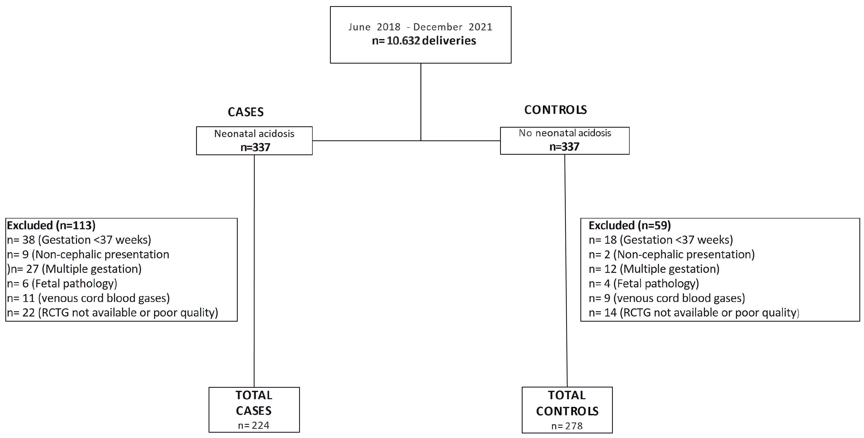
The study aimed to assess neonatal acidemia, characterized by a pH level less than 7.10 determined through arterial cord blood measurements at birth. Out of the initial cohort of 10,362 women, 337 infants (3.3%) were identified as acidotic. Figure 2 presents a flowchart outlining the study, where 113 acidemic fetuses were excluded from the analysis due to not meeting the criteria. Among the remaining participants, 224 infants with arterial acidemia were included as cases, while 278 infants were chosen as controls. The selection of the control group followed a non-randomized 1:1 consecutive method, where each selected control was chronologically consecutive to a case.

The study collected maternal and pregnancy data, including various factors such as maternal characteristics (e.g., age, nulliparity), type of labor, and neonatal characteristics (e.g., gestational age, birth weight, fetal gender, Apgar score at 5 min), as well as pH characteristics.

2.2. Electronic Fetal Monitoring

To ensure fetal well-being, a Corometrix 256CX fetal activity supervisor was used for monitoring. This involved the use of two sensors: an ultrasonic transducer for capturing the electrocardiographic (ECG) fetal activity and a Tocotonometer transducer for monitoring uterine activity. These sensors were securely attached to the mother using binding bands, allowing obstetricians to continuously analyze the signals from the later stages of pregnancy until delivery.

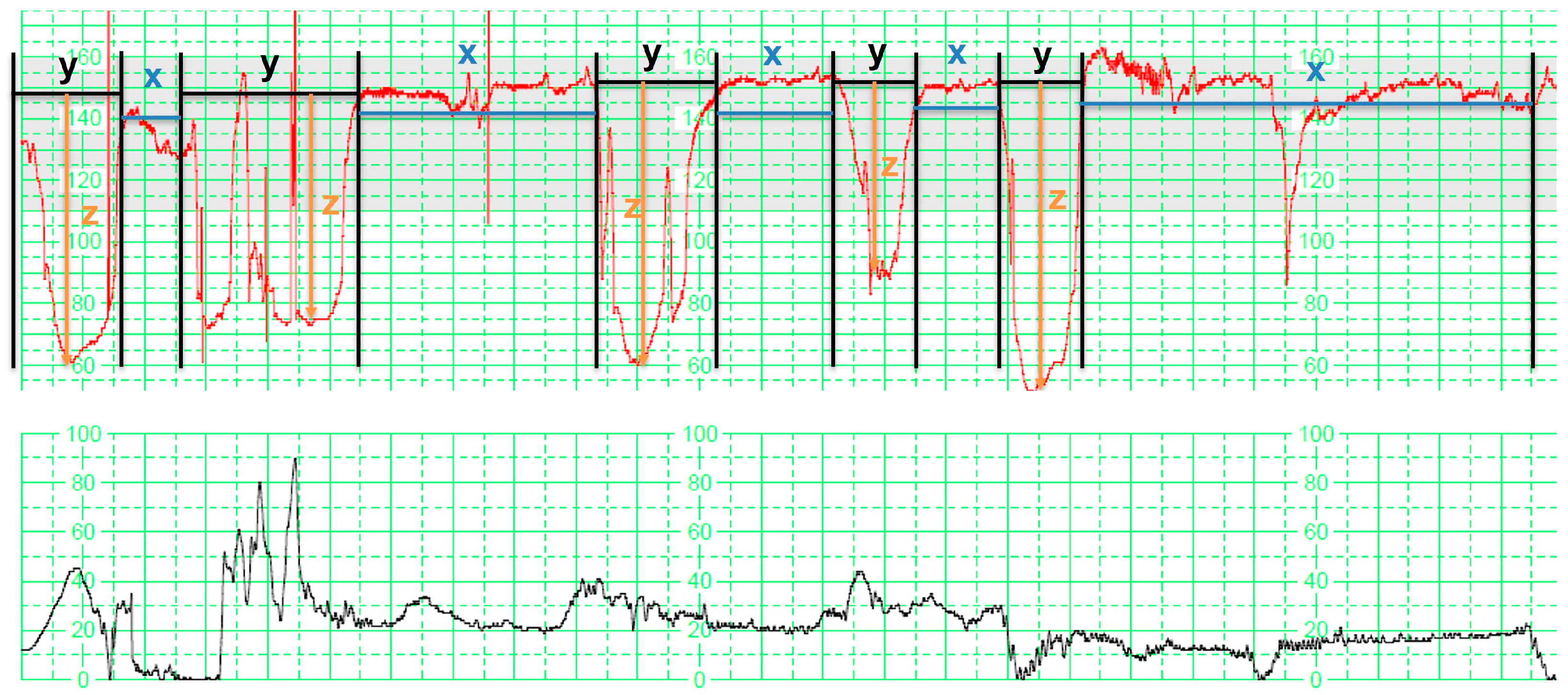
The analysis and interpretation of the EFM data from the last 30 min prior to delivery were performed by an expert obstetrician in the delivery section. The obstetrician, who was unaware of the neonatal outcome, assessed non-ACOG (NICHD) parameters. These parameters included total reperfusion time and deceleration area, which were measured during the 30 min preceding labor. Figure 3 shows the parameters required for their calculation.

The electronic fetal monitoring (EFM) signal was divided into two segments: deceleration (y) and interdeceleration (x). The interdeceleration period, referred to as x, represented the duration between decelerations. The duration of decelerations, denoted as y, represented the time during which decelerations occurred. The depth of decelerations was indicated as z. With these parameters (x, y, and z), the following measurements were computed:

• Total reperfusion time: This parameter was calculated by adding up the duration, measured in minutes, during which the fetus maintained a baseline state without any deceleration within the last 30 min (${\displaystyle \sum }_{i=1}^{n_x}{x}_i$), where $n_x$ is the total number of interdeceleration periods.
• Deceleration time: This parameter was determined by summing the duration, measured in minutes, of the period during which the fetus displayed decelerations within the last 30 min (${\displaystyle \sum }_{i=1}^{n_y}{y}_i$), where $n_y$ is the total number of deceleration periods.
• Total deceleration area: This parameter was computed by summing the areas of all the decelerations. Each deceleration’s area was determined by multiplying the duration of the deceleration in seconds by its maximum depth of fall from the baseline, given in beats per minute, and dividing the result by two (${\displaystyle \sum }_{i=1}^{n_y}{y}_i{z}_i/2$).

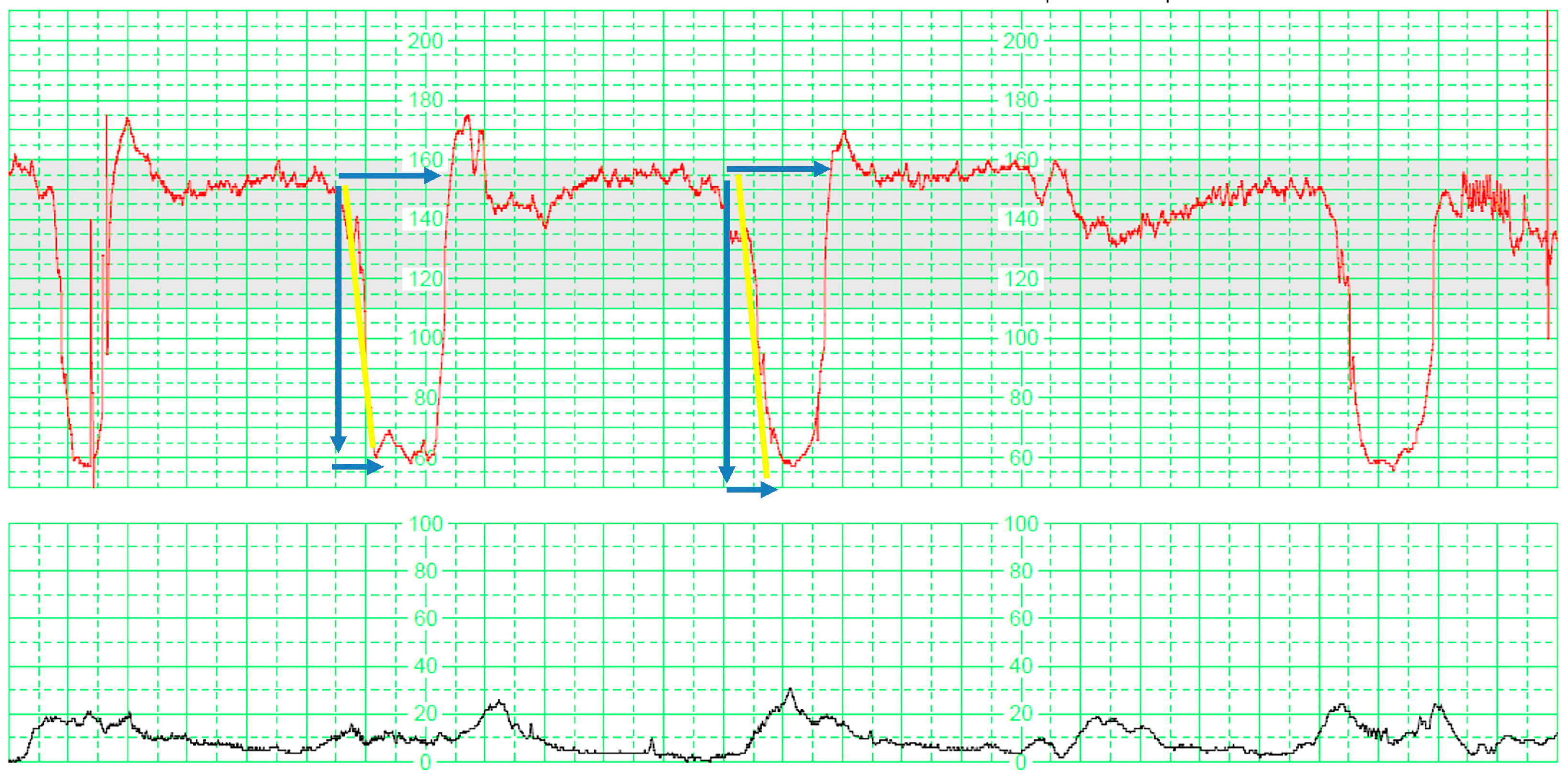
Additionally, various parameters related to the first and last decelerations were analyzed. These parameters encompassed amplitude, duration, drop, slope, area, fetal heart rate (FHR), excess of deceleration, deceleration instability, and reduced deceleration. The exploratory analysis revealed that the parameters associated with the last deceleration were more significant in predicting acidemia compared to those of the initial period. This finding aligns with the notion that information closer to delivery tends to be more informative. Consequently, only the parameters related to the last deceleration were considered. Furthermore, the study introduced the concept of parameter evolution by defining the difference between the last and first periods. A visual representation of the described parameters can be found in Figure 4.

2.3. Statistical Analysis

2.3.1. Model Building

A descriptive analysis of the data was performed to compare infants with acidosis and those without acidosis. Continuous variables were summarized using the median and interquartile range (IQR), while categorical variables were summarized using the absolute and relative frequency for each category. To assess the differences between the acidotic and non-acidotic groups for continuous and categorical data, the Mann–Whitney test or chi-square test was used, respectively.

To predict acidosis, various machine learning models were constructed, including logistic regression models, classification trees, random forest, one-hidden layer neural networks, and multi-layer perceptron neural networks. The original database was randomly divided into training (70%) and validation (30%) datasets to develop and evaluate these models. It was ensured that both groups had an equal proportion of acidotic cases.

The statistical analyses were conducted using the R programming language version 4.2.2 (The R Foundation for Statistical Computing, Vienna, Austria). Several libraries were utilized, including regplot, rpart, randomForestSRC, nnet, neuralnet, keras, and NeuralNetTools [39].

2.3.2. Model Validation

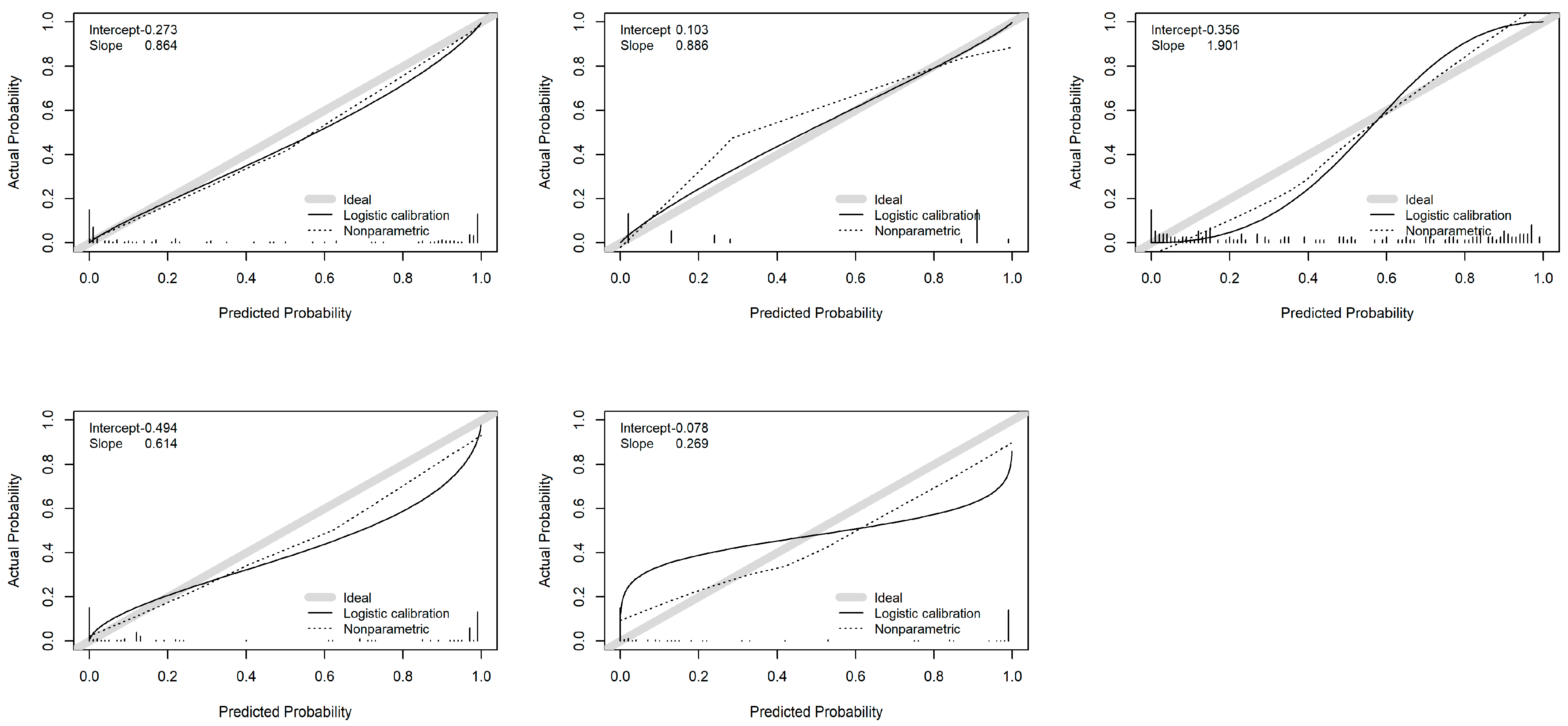
For the validation, the models were evaluated through calibration, discrimination, and clinical utility. The calibration curve was used to visually assess the agreement between predicted values and actual outcomes, with a diagonal line indicating perfect calibration. Additionally, two informative parameters, ‘intercept’ (calibration-in-the-large) and ‘slope,’ were examined. The ‘intercept’ quantifies the disparity between the average predictions and average outcomes, while the ‘slope’ indicates the average influence of predictions on the outcome [40].

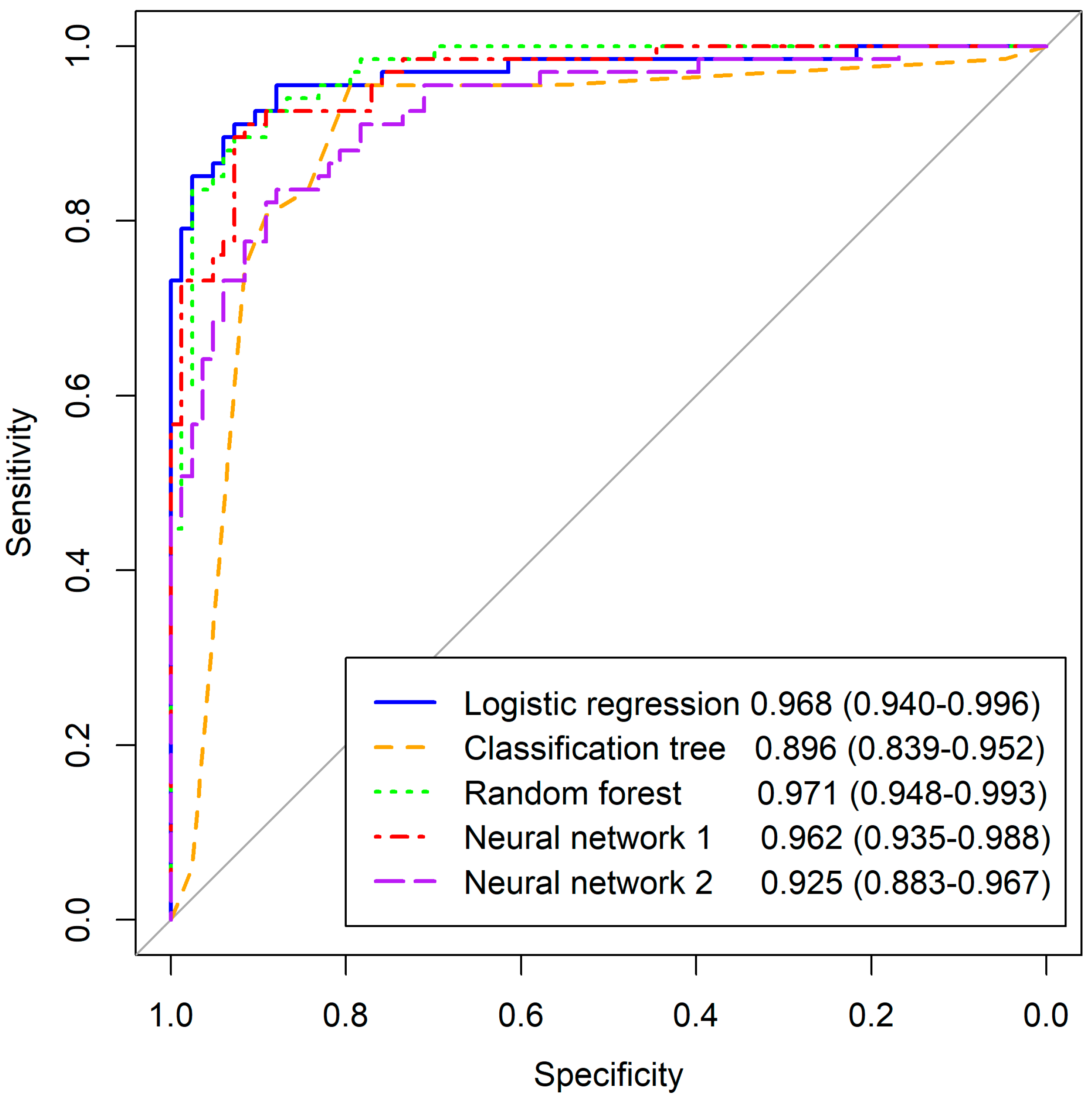
The discrimination was assessed using the receiver operating characteristic (ROC) curve. The ROC curve is a plot of pairs of sensitivity (true positive rate, y-axis) versus 1-specificity (false positive rate, x-axis) obtained for different cut-off values of acidemia probability. The area under the ROC curve (AUC) is a parameter that summarizes the discrimination ability of a predictive model. The AUC measures the probability that the model assigns a higher probability of being acidotic to an actual acidotic case compared to a non-acidotic case. It has a range of 0 to 1, where 0.5 indicates a random model, 0.7 is considered acceptable, 0.8 suggests a good model, 0.9 indicates an excellent model, and 1 represents perfect discrimination. The 95% confidence intervals for the AUC were calculated using DeLong estimation [41].

Furthermore, we investigated and compared the specificities for various sensitivities thresholds (0.8, 0.85, 0.9, 0.95) using a proportion test.

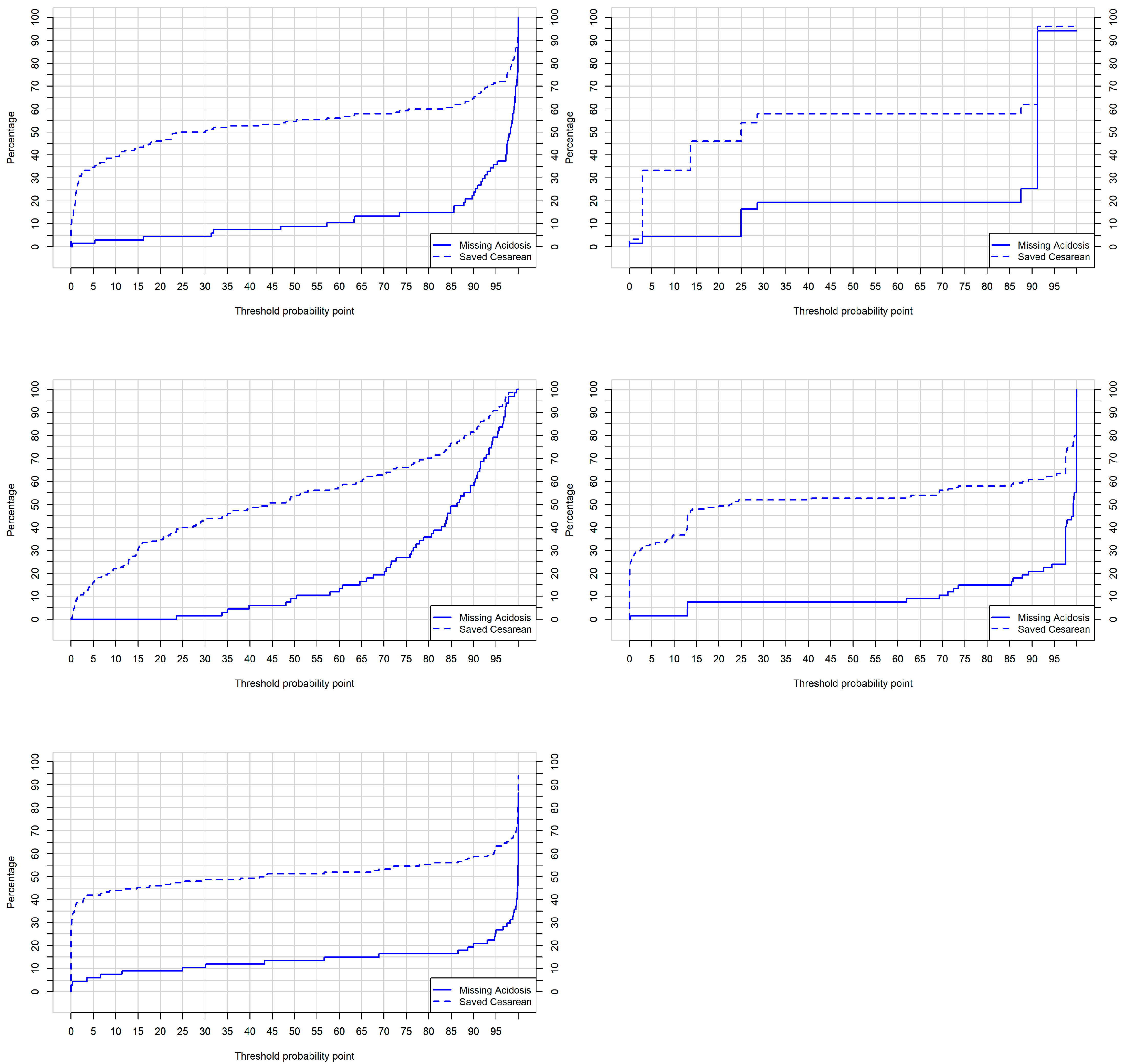
Additionally, we assessed the practical applicability of the developed machine learning models by evaluating their clinical usefulness. This evaluation involved treating the prediction models as dichotomous classification models, using a specific cutoff point to distinguish between positive (1) and negative (0) individuals above or below the threshold. To evaluate the clinical utility, we employed the clinical utility curve [42]. This curve utilizes the threshold probability on the x-axis to identify neonates as acidotic, while the y-axis represents the percentage of two distinct measures. The first measure indicates the percentage of acidotic infants that were incorrectly classified below the chosen cutoff point, and the second measure represents the number of infants falling below the cutoff point. By examining this curve for different cutoff points, we can determine the percentage of misclassified acidotic fetuses and the fetuses with a very low risk of acidemia who can be spared unnecessary cesarean sections due to fetal well-being concerns. These parameters are crucial in clinical practice.

The rms and pROC R libraries and the CUC R code function were used for validation purposes.

3. Results

3.1. Descriptive Characteristics

Table 1. Maternal characteristics and perinatal results.

	Total Sample n = 502	Non-Acidotic n = 278	Acidotic n = 224	p-Value
Maternal age	34 (30–37)	34 (30–36)	34 (30–37)	0.440
Nulliparity	302 (60.16%)	148 (53.24%)	149 (66.52%)	<0.001
Age gestational	280.5 (274–286)	280 (273.75–286)	281 (274.25–286)	0.205
Sex				0.87
Male	262 (52.19%)	146 (52.51)	116 (51.78)
Female	240 (47.81%)	132 (47.48)	108 (48.21)
Newborn percentile weight	3251.74 (471.07)	3281.09 (454.45)	3215.31 (489.34)	0.123
p < 10	73 (14.54)	30 (10.79%)	43 (15.47%)	0.011
>90	60 (11.95)	33 (11.87%)	27 (12.05%)	0.999
Birth eutocic	303 (60.36%)	193 (69.42%)	110 (49.11%)	<0.001
Instrumental delivery	121 (24.1%)	60 (21.58%)	61 (27.23%)	0.141
Cesarean section	78 (15.54%)	25 (8.99%)	53 (23.66%)	<0.001
Apgar 5 m < 7	36 (7.17%)	4 (1.44%)	32 (14.29)	<0.001
Umbilical arterial pH	7.12 (7.07–7.20)	7.18 (7.14–7.27)	7.06 (7.01–7.09)	<0.001
Umbilical venous pH	7.18 (7.13–7.22)	7.23 (7.18–7.26)	7.15 (7.09–7.19)	<0.001

provides an overview of the maternal and perinatal characteristics. We observed a higher prevalence of nulliparity in the acidotic group (p < 0.001). Fetal growth restriction was more frequently observed in the acidotic group (15.47%) compared to the non-acidotic group (10.79%), with statistically significant differences (p = 0.011). Additionally, the incidence of cesarean section was twice as high in the acidotic cases (23.66% vs. 8.99%). The median values of arterial and venous pH were 7.06 and 7.15, respectively, in the acidotic and non-acidotic groups, showing a significant difference (p < 0.001).

In

Table 2. Descriptive characteristics and prediction ability of the parameters of the study. bpm: beats per minute; FHR: fetal heart rate.

	Total n = 502	Non Acidotic n = 278	Acidotic n = 224	p-Value	Odds Ratio	AUC
30 min window
Deceleration range	14.16 (7.71, 22.54)	9.71 (5.37, 15.42)	20.93 (13.75, 28.65)	<0.001	1.141 (1.112, 1.171)	0.807
Reperfusion time	19.35 (15.37, 23.20)	21.69 (18.10, 25.12)	17.04 (13.86, 19.10)	<0.001	0.822 (0.787, 0.859)	0.750
Final deceleration window
Amplitude	72.99 (54.94, 87.04)	60.06 (49.96, 74.92)	84.87 (74.18, 95.11)	<0.001	1.063 (1.050, 1.076)	0.796
Duration	71.25 (59.88, 90.69)	61.8 (55.68, 89.92)	80.9 (64.32, 100.14)	<0.001	1.023 (1.015, 1.030)	0.670
Drop	32.63 (23.26, 46.51)	40.9 (30.79, 53.47)	23.96 (19.18, 32.32)	<0.001	0.933 (0.918, 0.947)	0.792
Slope	2.08 (1.31, 3.47)	1.57 (1.01, 2.05)	3.51 (2.49, 4.69)	<0.001	3.331 (2.681, 4.138)	0.853
Area	2.51 (1.89, 3.71)	2.15 (1.6, 2.72)	3.55 (2.45, 4.69)	<0.001	2.470 (2.048, 2.979)	0.781
FHR (bpm)	155 (145, 165)	150 (140, 160)	160 (150, 170)	<0.001	1.043 (1.029, 1.057)	0.664
Overshoot	67 (13.35%)	24 (8.63%)	43 (19.19%)	0.001	2.514 (1.473, 4.291)	0.552
Inestability	188 (37.45%)	50 (17.98%)	138 (61.61%)	<0.001	7.317 (4.867, 11.000)	0.718
Reduced variability	110 (21.9%)	38 (13.67%)	72 (32.14%)	<0.001	2.992 (1.922, 4.656)	0.592
Initial window
Amplitude (bpm)	6.12 (−1.97, 19.63)	4.16 (−4.11, 13.11)	12.32 (1.32, 24.38)	<0.001	1.023 (1.013, 1.034)	0.631
Duration (s)	2.15 (−7.31, 14.44)	1.31 (−4.71, 13.45)	3.90 (−8.76, 23.55)	0.136	1.008 (1.001, 1.015)	0.538
Drop (sg)	−1.41 (−10.84, 6.24)	−1.62 (−12.47, 8.11)	−0.78 (−8.72, 5.04)	0.611	1.001(0.991, 1.012)	0.513
Slope (bpm/sg)	0.29 (−0.24, 1.01)	0.24 (−0.22, 0.59)	0.64 (−0.29, 1.70)	<0.001	1.325 (1.154, 1.520)	0.599
Area (mm2)	32.41 (−19.11, 99.12)	17.20 (−25.10, 54.57)	70.28 (−1.05, 163.74)	<0.001	1.004 (1.003, 1.006)	0.657
FHR (bpm)	0 (0, 10)	0 (0, 5)	5 (0, 15)	<0.001	1.006 (1.004, 1.008)	0.651
Saltatory Pattern	88 (17.52%)	32 (11.51%)	56 (23.14%)	<0.001	2.643 (1.506. 4.638)	0.572

, we provide a comparative analysis of the deceleration area and reperfusion time measurements during the last 30 min of fetal ECG among the acidotic groups. We also present the parameters measured during the last deceleration of the fetal ECG and their difference from the first deceleration. Additionally, we include the odds ratio and the AUC of univariate logistic regression models for all predictor variables to predict acidosis.

The variables measured during the 30 min fetal monitoring window demonstrate good discriminatory ability. The deceleration area achieves an AUC value of 0.807, while the reperfusion time exhibits a slightly lower value of 0.750. When considering the parameters of the last deceleration, the slope of the deceleration demonstrates the highest AUC value of 0.853, surpassing those measured over the entire 30 min period.

3.2. Multivariate Prediction Models

In order to predict acidemia, we employed both conventional and machine learning approaches for classification problems. The conventional approach involved utilizing the stepwise logistic regression model. Additionally, we utilized machine learning algorithms such as classification trees, random forest, and artificial neural networks. Models were built using training data, and their discrimination, calibration, and clinical utility were estimated using validation data.

3.2.1. Logistic Regression

The construction of the logistic regression model involved a stepwise selection process, employing a backward/forward method. This iterative process involved removing variables based on an improvement in the Akaike index, while also considering the inclusion of variables that were removed from the model if their inclusion improved the index at any step.

Table 3. Multivariate logistic regression model.

	Odds Ratio (95% CI)	p-Value
30 min window
Deceleration area	1.121 (1.064, 1.189)	<0.001
Final deceleration window
Duration (s)	1.157 (1.117, 1.209)	<0.001
Drop (s)	0.809 (0.743, 0.871)	<0.001
Slope (bpm/sg)	2.814 (1.541, 5.523)	0.001
Difference between Final and Initial deceleration window
Duration (s)	0.950 (0.925, 0.974)	<0.001
(s)	1.133 (1.088, 1.188)	<0.001

displays the variables that were found to be statistically significant in the multivariate analysis.

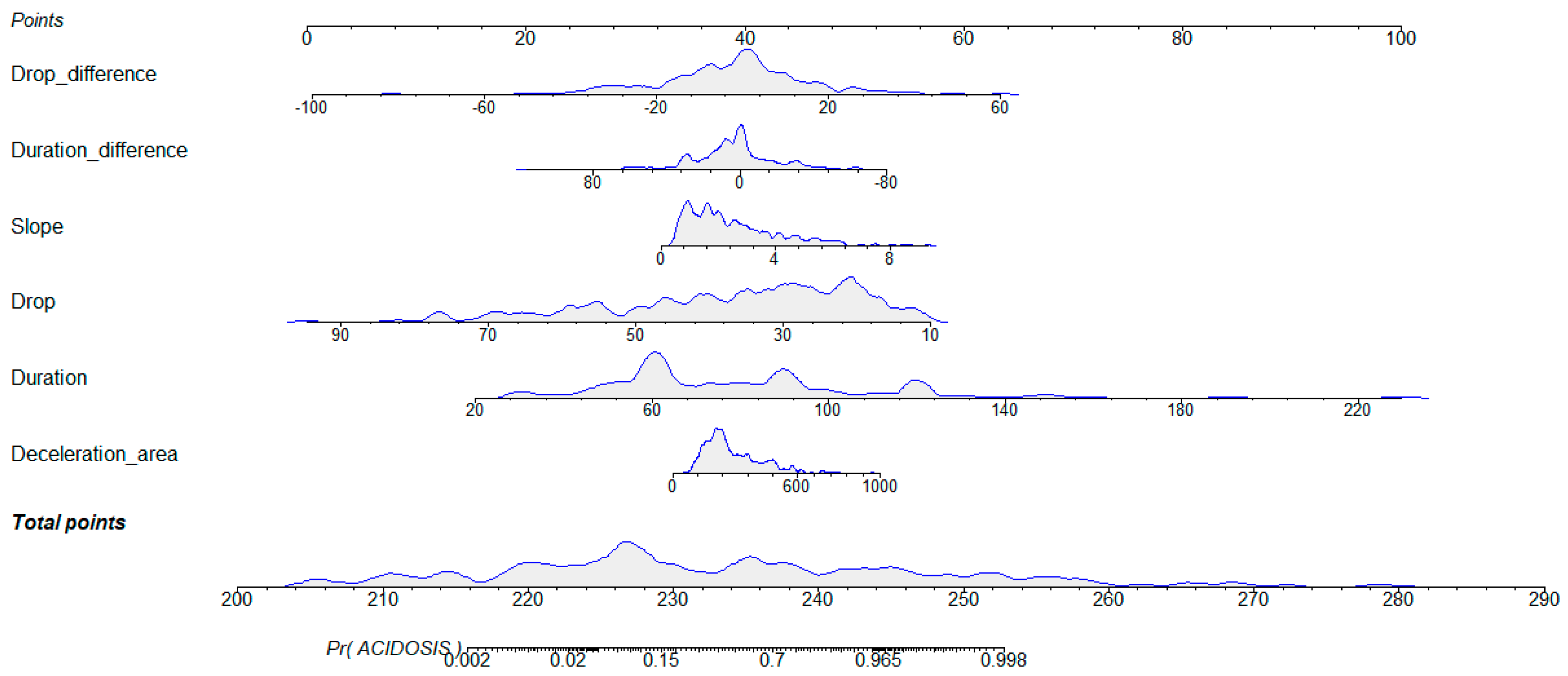
To illustrate the weight of the variables in the prediction model, we provide a nomogram in Figure 5. The nomogram shows the weight of variables in the model. For each individual, a score is assigned to each variable on the upper axis. By summing up these scores, a total score is obtained, which provides us with the probability of acidosis on the lower axis. Considering the variability of points assigned on the nomogram, the variables that show the most difference are the duration, the drop, and the drop difference. In these variables, we observe more variation among individuals, but both the drop and the drop difference do not yield very high scores compared to the drop. On the other hand, the duration difference, slope, and deceleration area exhibit reduced variability, but due to their high scores, even slight variations within their range can be highly significant in providing a high probability of acidosis.

3.2.2. Classification Trees

Classification trees are recursive partition models that minimize the impurity of the classes defined by the partition. They provide a simple classification system that is easy to implement, but they often lack high discrimination ability. In this study, we used the Gini index as the loss function and set the minimum number of observations required for a split to 20 in a node. Additionally, we set the minimum number of observations in any terminal node to seven and limited the maximum depth of any node in the final tree to 30. Figure 6 displays the classification tree.

The slope is the variable that best discriminates in the first node, followed by the duration of the deceleration on the second level, and the duration for the left branch or the reperfusion time for the right branch in the third level. To assess the impact of predictor variables on acidemia prediction, we present the variable importance (VIMP) plot in Figure 7. The VIMP quantifies the difference in prediction error when a predictor is perturbed by applying a permutation that assigns the variable to a terminal node different from its original assignment. These calculations are performed for each tree in the model, resulting in the Breiman–Cutler Variable VIMP [43]. The three variables that exerted the most influence on acidemia prediction were the slope, the drop, and the duration of the last deceleration window.

3.2.3. Random Forest

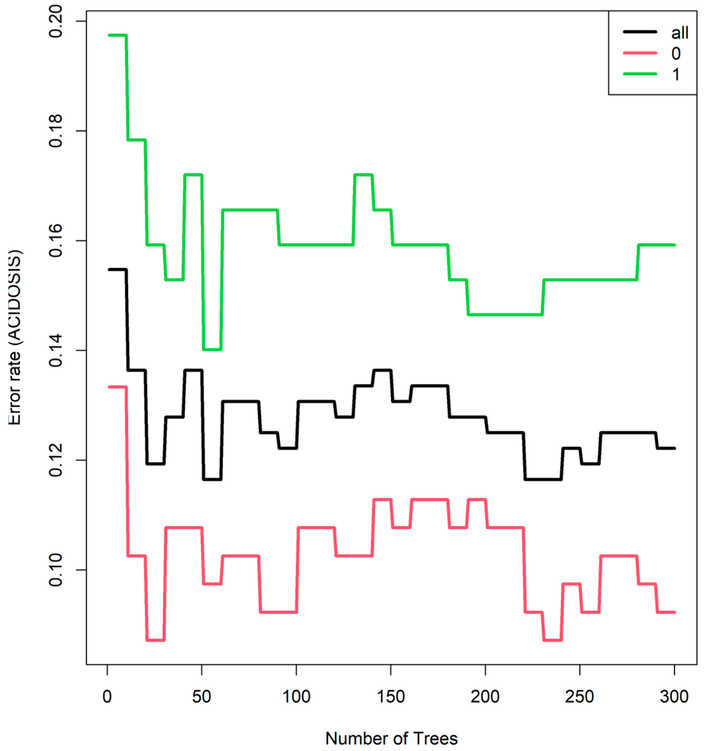
Random forests consist of an ensemble of classification trees, where each tree is trained using a unique bootstrap sample and a different combination of variables. This approach ensures diversity among the trees, resulting in a more robust model. For our analysis, we utilized a sample size of 222, which corresponds to approximately 60% of the total data, to build each tree. The splitting rule employed was Gini, and we considered 10 random split points. Furthermore, we added a total of 300 trees to the ensemble, as this number was found to be reasonable based on the reduction in prediction error depicted in Figure 8. The error rate was evaluated for the non-acidotic cases (0), acidotic cases (1), and all data, using the out-of-bag (OOB) error estimation. The data not used for building each tree were used to estimate prediction error, and an average prediction error was estimated.

To optimize the terminal node size of the forest and the number of variables used to train each tree, we employed a tuning optimization parameter. The results of this optimization are depicted in Figure 9. The best-performing model was achieved with a minimum size of three for the terminal node and by training each tree with six variables.

Figure 10 illustrates the variable importance in the random forest, highlighting the most significant variables. It is noteworthy that in a more robust model like the random forest model, the importance of the slope in the last deceleration window becomes increasingly prominent.

3.2.4. Neuronal Networks

We utilized two distinct neural networks for training purposes. The first network employed a classical perceptron architecture with a single hidden layer. The neural network was trained with different architectures, using different random initial weights and training parameters. We experimented with learning rates of 0.05 and 0.1, and used the hyperbolic tangent (tanh) and logistic activation functions.

$$\tanh \left(x\right)=\frac{e^x-e^{-x}}{e^x+e^{-x}}; \mathrm{logistic}\left(x\right)=\frac{1}{1+e^{-x}}$$

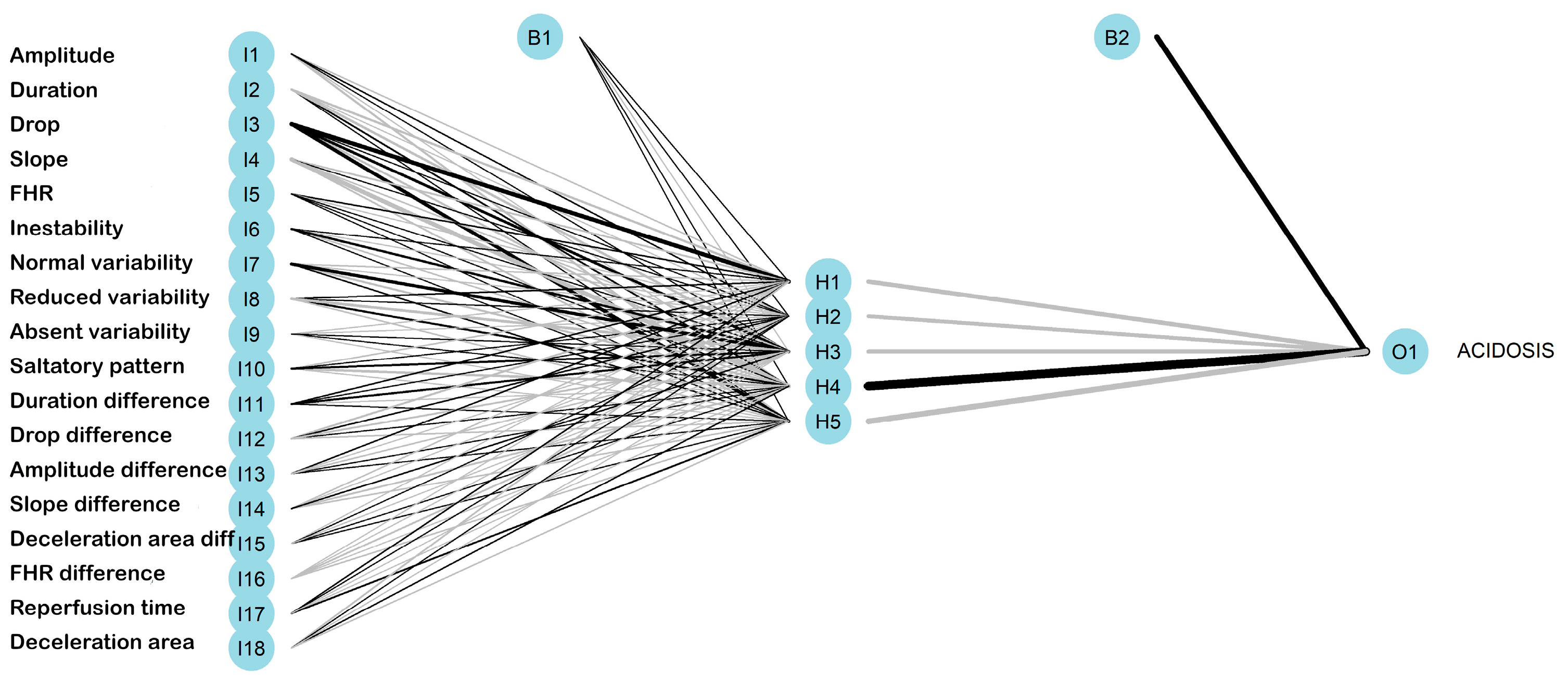
The best model was attained using an architecture of 18-5-1, indicating 18 input nodes, 5 nodes in the hidden layer, and 1 output node. A total of 101 weights were estimated, and the logistic activation function was used. The optimization function employed was cross-entropy, which measures the disparity between predictions and the actual occurrence of acidemia. The architecture of the network is visually represented in Figure 11, with positive weights depicted as black lines and negative weights shown as grey lines. The thickness of each line corresponds to the relative magnitude of the weight it represents.

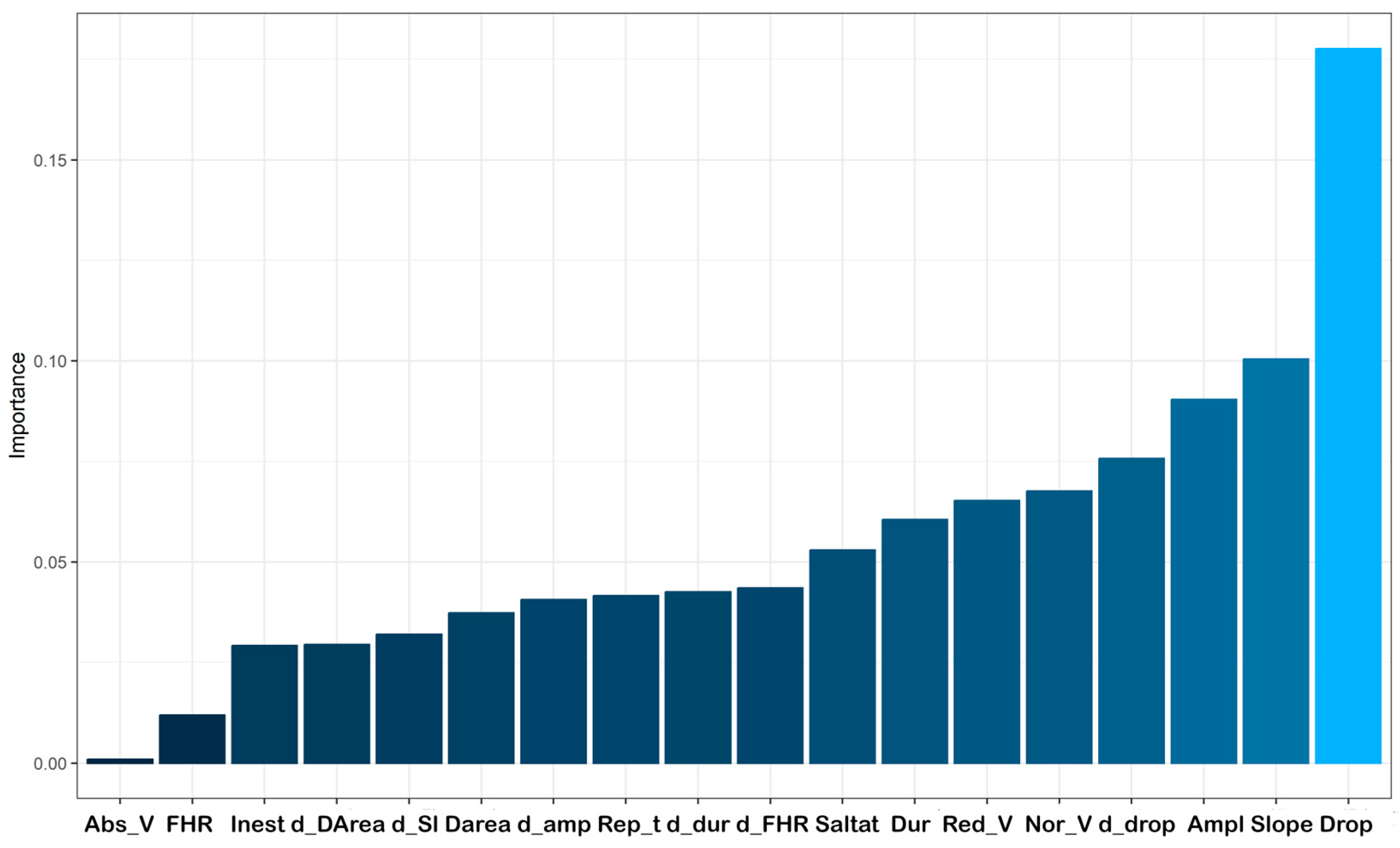
Figure 12 illustrates the variable importance plot for the multilayer perceptron, utilizing the methodology proposed by Garson in 1991 [44]. This approach involves deconstructing the model weights to determine the relative importance of explanatory variables for a single response within a supervised neural network. The variables that exerted the greatest influence were the drop, slope, and duration of the last deceleration time window. It is noteworthy that, contrary to expectations, the drop in the deceleration, rather than the slope, emerged as the most significant variable in this model.

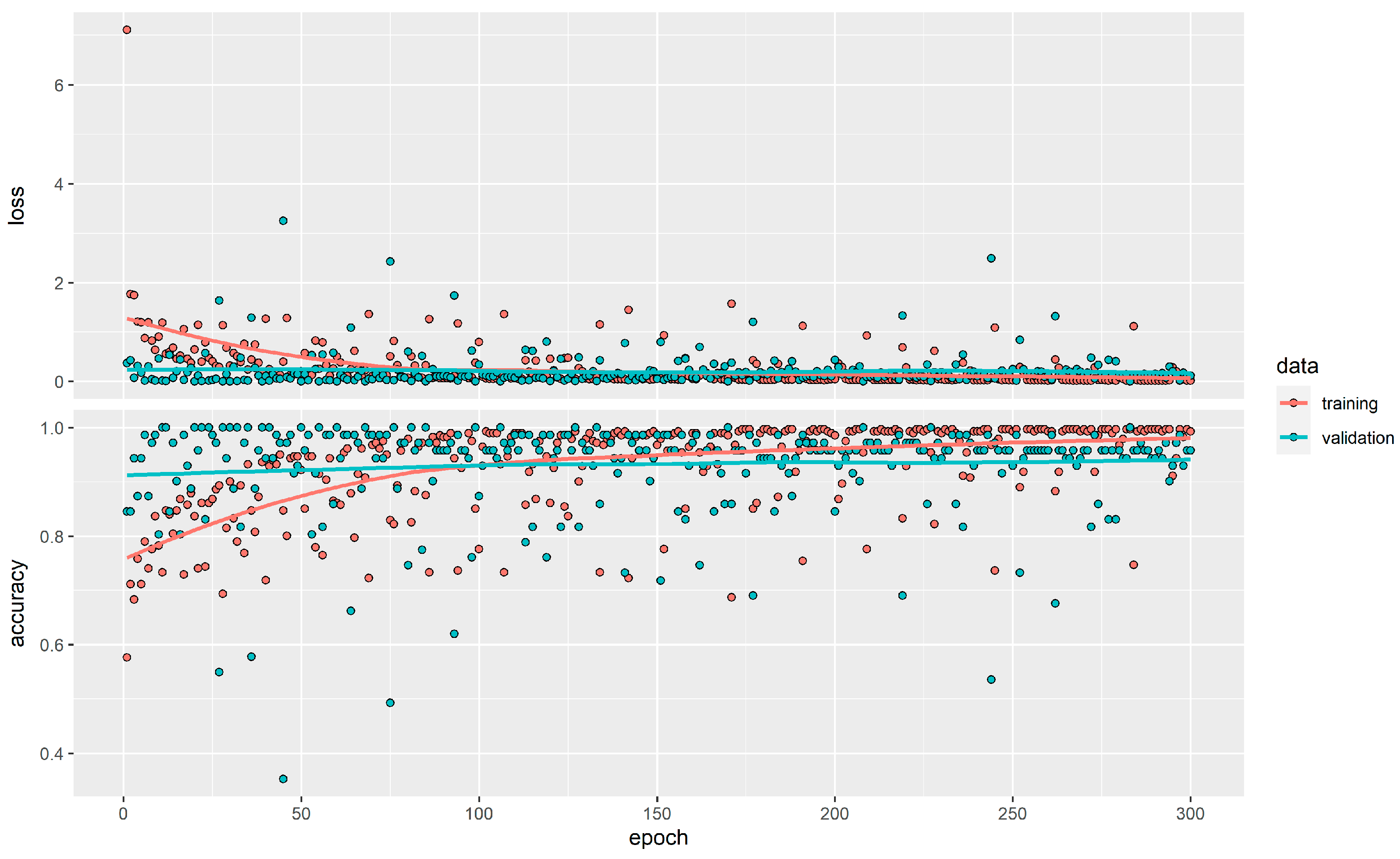
Additionally, a multilayer perceptron with two hidden layers was trained. We explored as an activation function the ReLU $f\left(x\right)=\left\{\begin{array}{c}x if x>0\\ 0 if x\le 0\end{array}\right.$, linear $f\left(x\right)=x$, and sigmoid $f\left(x\right)=\frac{1}{1+e^{-x}}$, the learning rate was fixed as 0.01, the number of epochs xplored ranged from 20 to 400, and the number of units of the hidden layer was set as 32, 64 or 128. The architecture of the best network was 16-64-32-2, with 3234 weights estimated. The activation function for the first and second hidden layers was ReLU, and softmax was used for the output layer. The loss function employed was categorical crossentropy, with the optimizer set as rmsprop, and the metric used for optimization was accuracy. The model was trained for 30 epochs, with a batch size of 128, and a validation split of 0.2 was used to estimate the convergence, as shown in Figure 13. Due to the complexity of this model, it is not graphically represented.

3.3. Validation of Developed Models

To evaluate the validity of the models, we utilized a separate set of validation data comprising 30% of the total dataset. This approach allowed us to assess the performance of the machine learning models on data that were not used during the model development phase.

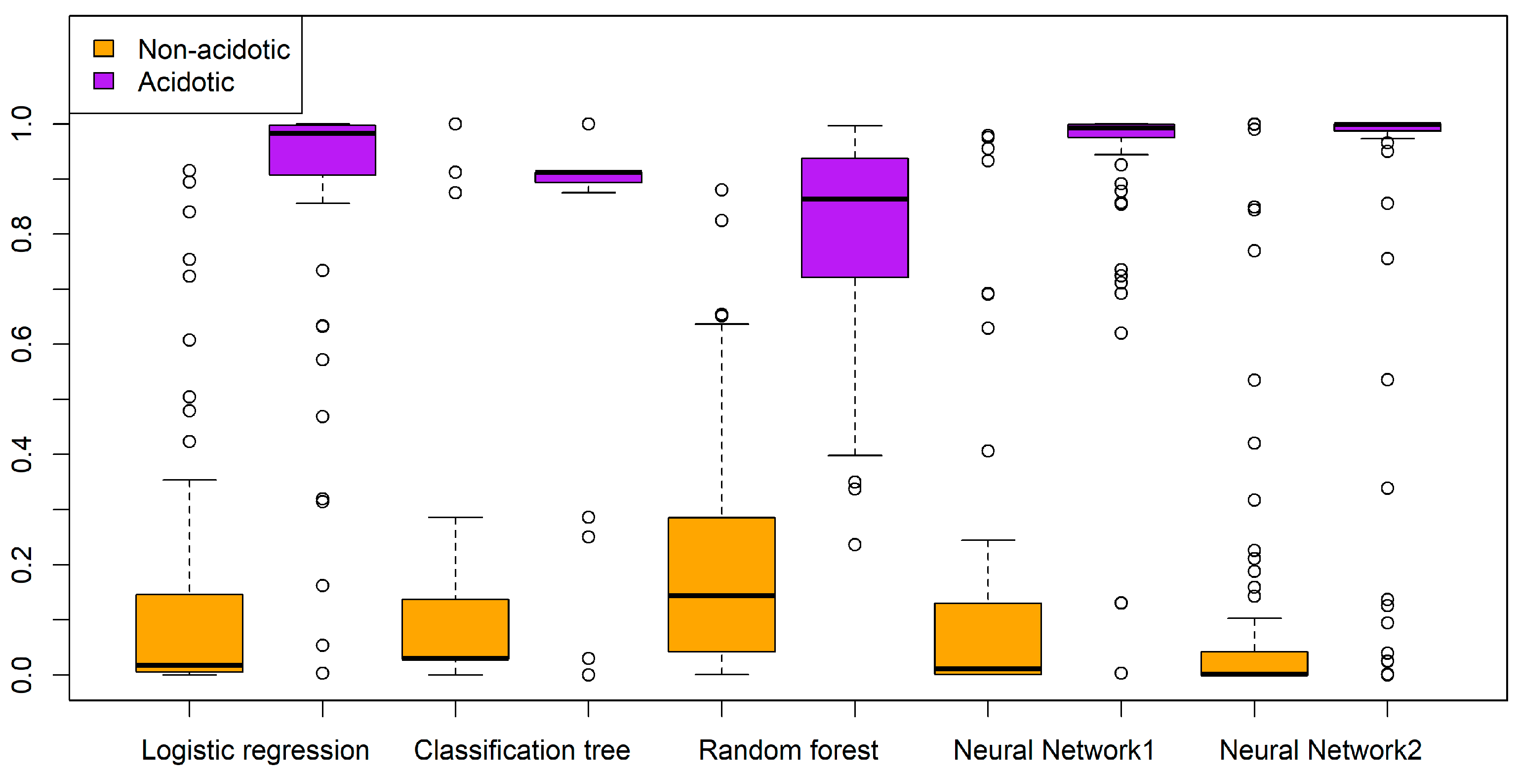
Regarding the probabilities provided by the models, we presented their distribution in a comparative boxplot in Figure 14. All models exhibited a high discrimination ability. The random forest and logistic regression models provided probabilities for acidotic cases distributed across a wide range, while the neural network models produced probabilities confined to a narrower range.

The calibration of the models is in accordance with the analyzed distribution of probabilities. Figure 15 displays calibration curves, where the x-axis corresponds to the predicted probabilities and the y-axis represents the actual occurrence of acidosis. The logistic regression and classification tree models demonstrate good calibration. However, the random forest model tends to overestimate low probabilities and underestimate high probabilities. The perceptron with one hidden layer tends to overestimate high probabilities, while the two-hidden-layer neural network underestimates low probabilities and overestimates high probabilities.

Regarding the discrimination ability, all models exhibit excellent discrimination with AUC values very close to or above 0.9. The highest AUC is achieved by the random forest model with an AUC of 0.971 (0.948, 0.993), which shows no statistically significant difference compared to the logistic regression model (0.968 (0.940, 0.996), p = 0.846), the neural network with one hidden layer (0.962 (0.35, 0.988), p = 0.352), or the neural network with two hidden layers (0.925 (0.883, 0.967), p = 0.063). However, the random forest model demonstrates superiority over the classification tree model (0.896 (0.839, 0.952), p = 0.004). The ROC curves are displayed in Figure 16.

Although we observed similar behavior in terms of AUC values, it is crucial for the predictive models to be effective in detecting acidotic cases, especially at high sensitivity values.

Table 4. Specificities for sensitivities values.

Specificities	Logistic Regression	Classification Tree	Random Forest	Neural Network 1	Neural Network 2
0.80	0.976	0.894	0.976	0.928	0.892
0.85	0.976	0.837	0.952	0.928	0.831
0.90	0.928	0.817	0.892	0.916	0.783
0.95	0.879	0.797	0.831	0.771	0.710

summarizes the specificities for high sensitivity values. When considering a sensitivity value of 0.9, the logistic regression model performs the best with a specificity of 0.928. It is followed by the neural network with one hidden layer (0.916, p = 0.712), random forest (0.892, p = 0.182), classification tree (0.817, p < 0.001), and the neural network with two hidden layers (0.782, p < 0.001).

In order to effectively prioritize the identification of acidotic cases, our study emphasizes logistic regression, random forest, and one-hidden-layer perceptron as the most optimal models. However, a crucial question remains: to what extent can these models help reduce the number of unnecessary cesarean sections? This important aspect can be examined by analyzing the clinical utility curves presented in Figure 17. The x-axis represents the potential threshold acidosis probability points used to classify individuals as acidotic or non-acidotic. On the y-axis, we present the percentage of acidosis cases misclassified below the selected cut-off point (indicated by a solid line) and the percentage of cesarean sections that could be avoided (depicted with a dotted line).

By analyzing the clinical utility curve, we can determine the number of cesarean sections that could be avoided by detecting a certain percentage of acidemia cases. For example, when there is a 10% misclassification rate of acidemia cases, the logistic regression and one-hidden-layer neural network models are able to avoid 56% of unnecessary cesarean sections. The random forest model closely follows with a rate of 54% (p = 0.566), while the two-hidden-layer neural network and classification tree models have lower rates of 48% (p = 0.013) and 46% (p = 0.002), respectively.

4. Discussion

In this study, we performed a comparative analysis of different machine learning techniques to predict acidemia using fetal heart rate features obtained from continuous electronic fetal monitoring during the last 30 min of the intrapartum period. Our predictor variables included reperfusion time and deceleration time measured over the entire 30 min period. Furthermore, we examined parameters of the last deceleration and their changes within the 30 min timeframe. The slope of the last deceleration was found to be the most predictive parameter, which has previously been studied in animal models.

Regarding FHR parameters related to acidosis, Shelley et al. (1971) [45] demonstrated an inverse correlation between deceleration area, umbilical pH, and Apgar score at 1 min. Beguin et al. (1975) [46] found a correlation between deceleration area and fetal pH values. Tranquili et al. (2013) [47] established a correlation between the area of fetal bradycardia and the timing of acidemia, although their results were based on a small sample size of thirty acidemic infants. Hamilton et al. (2011) [48] introduced the “sixty rule”, which stated that decelerations with a depth below 60 bpm and lasting more than 60 s were more discriminatory for metabolic acidemia. Cahill et al. (2018) [8] reported that a persistent 10 min period of category III decelerations was significantly associated with acidemia. However, most records were classified as category II, and there was no association with neonatal acidemia, despite achieving a better AUC (0.64) than category III. Furukawa et al. (2019) [49] compared computerized systems and reported that deceleration area was the best parameter for predicting neonatal acidemia.

Logistic regression has been commonly used as a machine learning technique to combine FHR parameters. Marti et al. (2018) [7] found that ACOG parameters such as minimal variability, the total number of late decelerations, prolonged decelerations, and total deceleration area showed high discrimination power. Combining deceleration area with maternal–fetal characteristics, they achieved a good discrimination ability of 0.83. Cahill et al. (2018) [8] obtained similar results, where a combination of total deceleration area, ever tachycardic, and ever moderate variability resulted in an AUC of 0.77.

Choliz-Ezquerro et al. (2022) [9] analyzed the total reperfusion time or inter-deceleration time, which is crucial in assessing fetal oxygenation. They combined this parameter with the number of decelerations, the number of decelerations greater than 60 s, the number of decelerations greater than 60 beats per minute, the number of recurrent decelerations greater than 60 beats per minute, the minimum depth of beats per minute, maternal parity, and fetal weight that is large for gestational age. Although this model has higher accuracy with an AUC of 0.826, it includes specific variables that may limit its clinical use. In fact, they recommended using only the reperfusion time with a cutoff of 23.75 min in 30 min (sensitivity of 90%, negative predictive value of 89%).

Understanding the normal fetal physiological compensation response is crucial for accurately interpreting features observed in electronic fetal monitoring (EFM). EFM should be viewed as a dynamic process rather than a static classification based on morphological features [50].

The effectiveness of electronic fetal monitoring (EFM) as a predictor of fetal acidemia has been the subject of criticism, and concerns have been raised regarding its medical and legal implications [51]. Studies have shown that the total deceleration area and reperfusion time are superior predictors of fetal acidemia compared to the ACOG category III classification when considered as independent parameters. However, to achieve the best prediction, these parameters may need to be combined with other EFM, fetal, or maternal variables. This raises doubts about the validity of the current category system in existing EFM guidelines.

Therefore, it is necessary to reevaluate and question the relevance and effectiveness of the current category system in EFM guidelines. Alternative approaches, such as incorporating total deceleration area and reperfusion time along with other relevant variables, should be explored to improve the prediction of fetal acidemia.

Experimental studies conducted on term sheep fetuses have confirmed that extending the series of cordal occlusions leads to an increase in the slope of decelerations. This effect is more pronounced and observed more frequently in cases of severe acidosis [11].

The advancement of data extraction and monitoring devices necessitates the development of new software for analyzing fetal heart rate (FHR) data. With the digitalization of the FHR signal, it becomes feasible to process it using convolutional neural networks (CNNs) or more complex encoder–decoder deep learning architectures for acidemia prediction. In the work by Tang [38], the MKNet model is introduced, which utilizes a CNN and achieves an impressive AUC value of 0.95. The author suggests its application in real-time fetal health monitoring using portable devices. Similarly, Zhao [16] also employs a CNN approach and achieves an AUC above 0.95 through a 10-fold cross-validation procedure for prediction purposes. Computer-aided diagnosis systems have shown lower predictive ability; Cömert [15] found a sensitivity of 76.83% and specificity of 78.27%, although Anisha [26] demonstrated an AUC of 0.96 for detecting cardiac anomalies. Despite the high accuracy demonstrated by some models, there is a lack of research on their clinical utility.

An alternative approach involves extracting variables from the fetal heart rate (FHR) signal and incorporating them into binary classification models for acidemia prediction. In our analysis, we trained logistic regression, classification trees, random forest, and neural networks using readily available FHR features as predictor variables from the electronic fetal monitoring (EFM) recordings. Among these models, the random forest algorithm demonstrated the highest performance in terms of AUC. The random forest model, known for its additive nature, provides robust predictions by combining multiple trees constructed with diverse sets of data and variables. In our study, the optimal model was achieved using 300 trees, with each tree exploring the predictive capacity of variables on different data samples. To prevent overfitting, we limited the number of cases at a terminal node to a maximum of three in each tree.

Although the AUC is the most commonly used parameter to validate a predictive model, in practice, we need to correctly classify a high percentage of acidemia cases. Therefore, we are interested in the points on the ROC curve that correspond to high sensitivity. In this case, logistic regression was the best model, only failing to classify 5% of acidemia cases, achieving a specificity of 87.9%. However, our models demonstrated good accuracy overall.

In terms of calibration analysis, logistic regression and random forest models showed well-distributed probabilities of acidemia across a wide range of values. In contrast, neural networks exhibited probabilities concentrated near 0 and 1, indicating overfitting. This concentration made it difficult to determine a suitable threshold probability for distinguishing acidotic and non-acidotic cases. Logistic regression and random forest models, being more robust, allowed for a detailed analysis of the trade-offs between misclassifications and avoided cesarean sections.

Notably, the logistic regression model demonstrated promising results by potentially preventing 51% of unnecessary deliveries while experiencing only a minimal 5% loss in correctly identifying acidotic cases.

In a similar vein, Zhao [16] employed an AdaBoost model that achieved a sensitivity of 92% and specificity of 90%, which closely aligns with our findings, emphasizing the robustness of additive tree models. However, no information is available regarding the potential reduction in cesarean sections through the misclassification of acidosis cases. Iraji [38], on the other hand, achieved near-perfect classification results using neural networks, with a sensitivity of 99% and specificity of 97%. Nevertheless, these exceptionally high values would benefit from external validation for further confirmation.

In a meta-analysis conducted by Balayla [52], it was concluded that the use of AI and computer analysis for EFM interpretation during labor does not improve neonatal outcomes. However, their conclusions were solely based on risk ratio analysis. As illustrated in our study, while overall accuracy measures such as AUC may indicate comparable model performance, a comprehensive validation process is essential to thoroughly assess their effectiveness.

The strength of our study lies in the development of a classification model utilizing machine learning algorithms applied to EFM features. Specifically, we combined a 30 min period with variables extracted from the last deceleration before delivery and their progression over the subsequent 30 min. These predictor variables have previously exhibited promising predictive capabilities for acidemia. However, few studies have integrated them into a comprehensive predictive model utilizing various machine learning algorithms. Moreover, our model demonstrated favorable clinical utility, making it applicable in real-world clinical practice.

However, our study does have certain limitations. It was conducted retrospectively and relied on data from a single hospital, thus necessitating external validation on a larger scale for wider application.

5. Conclusions

By utilizing FHR recordings, we have successfully developed machine learning models for predicting acidemia. These models have demonstrated favorable accuracy, with an AUC ranging from 0.896 for the classification tree, 0.926 and 0.962 for the two- and one-hidden-layer neural networks, 0.968 for the logistic regression, to 0.971 for the random forest model in the validation dataset. Given the critical importance of accurately detecting acidosis, which is related to fetal hypoxia, the best model can be considered the one that corresponds to a very high rate of acidemia detection. When aiming for a sensitivity of 90%, the specificities ranged from 0.783 for the two-hidden-layer neural network to 0.817 for the classification tree, 0.892 for the random forest, 0.916 for the one-hidden-layer neural network, to 0.879 for the logistic regression model. For a sensitivity of 95%, the specificity of the neural network decreased to 0.771, while the logistic regression model maintained the highest specificity value of 0.879. Therefore, the logistic regression model can be considered the best and most robust model for predicting acidosis.

We combined previously explored parameters, such as deceleration within the 30 min window, with new parameters derived from the last deceleration (slope, drop, duration, variation in duration, and drop), resulting in a highly accurate predictive model and a user-friendly nomogram for their use. These variables can be routinely extracted from the FHR signal, providing a practical tool for healthcare professionals. In clinical practice, the nomogram provided by the logistic regression model can be implemented with a cutoff point of 31% probability for acidemia. This threshold minimizes the occurrence of missed acidemia cases (5%) while effectively preventing unnecessary cesarean sections in 51% of cases.

Overall, our study demonstrates the effectiveness of machine learning models in predicting acidemia using FHR recordings. The logistic regression model, along with the developed nomogram, offers a valuable and user-friendly tool for healthcare providers to make informed decisions and improve fetal health outcomes.

References

1. Nunes, I.; Ayres-de-Campos, D. Computer analysis of foetal monitoring signals. Best Pract. Res. Clin. Obstet. Gynaecol. 2016, 30, 68–78. [Google Scholar] [CrossRef]
2. Clark, S.L.; Hamilton, E.F.; Garite, T.J.; Timmins, A.; Warrick, P.A.; Smith, S. The limits of electronic fetal heart rate monitoring in the prevention of neonatal metabolic acidemia. Am. J. Obstet. Gynecol. 2017, 216, 163.e1–163.e6. [Google Scholar] [CrossRef] [PubMed] [Green Version]
3. American College of Obstetricians and Gynecologists. Fetal heart rate monitoring: Guidelines. ACOG Tech. Bull. 1974, 32, 1–10. [Google Scholar]
4. American College of Obstetricians and Gynecologists. Practice bulletin no. 116: Management of intrapartum fetal heart rate tracings. Obstet. Gynecol. 2010, 116, 1232–1240. [Google Scholar] [CrossRef] [PubMed]
5. Zamora, C.; Chóliz, M.; Mejía, I.; Díaz de Terán, E.; Esteban, L.M.; Rivero, A.; Castán, B.; Andeyro, M.; Savirón, R. Diagnostic capacity and interobserver variability in FIGO, ACOG, NICE and Chandraharan cardiotocographic guidelines to predict neonatal acidemia. J. Matern. Fetal Neonatal Med. 2021, 80, 6479. [Google Scholar]
6. Rei, M.; Tavares, S.; Pinto, P.; Machado, A.P.; Monteiro, S.; Costa, A.; Costa-Santos, C.; Bernardes, J.; Ayres-De-Campos, D. Interobserver agreement in CTG interpretation using the 2015 FIGO guidelines for intrapartum fetal monitoring. Eur. J. Obstet. Gynecol. Reprod. Biol. 2016, 205, 27–31. [Google Scholar] [CrossRef] [PubMed]
7. Martí, S.; Lapresta, M.; Pascual, J.; Lapresta, C.; Castán, S. Deceleration area and fetal acidemia. J. Matern. Fetal Neonatal Med. 2017, 30, 2578–2584. [Google Scholar] [CrossRef] [Green Version]
8. Cahill, A.G.; Tuuli, M.G.; Stout, M.J.; López, J.D.; Macones, G.A. A prospective cohort study of fetal heart rate monitoring: Deceleration area is predictive of fetal acidemia. Am. J. Obstet. Gynecol. 2018, 218, 523.e1–523.e12. [Google Scholar] [CrossRef]
9. Chóliz, M.; Savirón, R.; Esteban, L.M.; Zamora, C.; Espiau, A.; Castán, B.; Castán Mateo, S. Total intrapartum fetal reperfusión time (fetal resilience) and neonatal acidemia. J. Matern. Fetal Neonatal Med. 2021, 91, 5977. [Google Scholar]
10. Bennet, L.; Gunn, A.J. The fetal heart rate response to hypoxia: Insights from animal models. Clin. Perinatol. 2009, 36, 655–672. [Google Scholar] [CrossRef]
11. Westgate, J.A.; Wibbens, B.; Bennet, L.; Wassink, G.; Parer, J.T.; Gunn, A.J. The intrapartum deceleration in center stage: A physiologic approach to the interpretation of fetal heart rate changes in labor. Am. J. Obstet. Gynecol. 2007, 197, e1–e11. [Google Scholar] [CrossRef] [PubMed]
12. Sbrollini, A.; Agostinelli, A.; Marcantoni, I.; Morettini, M.; Burattini, L.; Di Nardo, F.; Fioretti, S.; Burattini, L. eCTG: An automatic procedure to extract digital cardiotocographic signals from digital images. Comput. Methods Programs Biomed. 2018, 156, 133–139. [Google Scholar] [CrossRef]
13. Doret, M.; Helgason, H.; Abry, P.; Goncalves, P.; Gharib, C.; Gaucherand, P. Multifractal analysis of fetal heart rate variability in fetuses with and without severe acidosis during labor. Am. J. Perinatol. 2011, 28, 259–266. [Google Scholar] [CrossRef] [PubMed] [Green Version]
14. Doret, M.; Spilka, J.; Chudáček, V.; Gonçalves, P.; Abry, P. Fractal analysis and hurst parameter for intrapartum fetal heart rate variability analysis: A versatile alternative to frequency bands and LF/HF ratio. PLoS ONE 2015, 10, e0136661. [Google Scholar] [CrossRef] [Green Version]
15. Cömert, Z.; Kocamaz, A.F. Open-access software for analysis of fetal heart rate signals. Biomed. Signal Process. Control 2018, 45, 98–108. [Google Scholar] [CrossRef]
16. Zhao, Z.; Zhang, Y.; Deng, Y. A comprehensive feature analysis of the fetal heart rate signal for the intelligent assessment of fetal state. J. Clin. Med. 2018, 7, 223. [Google Scholar] [CrossRef] [PubMed] [Green Version]
17. Esteban-Escaño, J.; Castán, B.; Castán, S.; Chóliz-Ezquerro, M.; Asensio, C.; Laliena, A.R.; Sanz-Enguita, G.; Sanz, G.; Savirón, R. Machine learning algorithm to predict acidemia using electronic fetal monitoring recording parameters. Entropy 2022, 24, 68. [Google Scholar] [CrossRef]
18. Ayres-de-Campos, D.; Nogueira-Reis, Z. Technical characteristics of current cardiotocographic monitors. Best Pract. Res. Clin. Obstet. Gynaecol. 2016, 30, 22–32. [Google Scholar] [CrossRef]
19. Docker, M. Doppler ultrasound monitoring technology. BJOG Int. J. Obstet. Gynaecol. 1993, 100, 18–20. [Google Scholar] [CrossRef]
20. Nunes, I.; Ayres-de-Campos, D.; Figueiredo, C.; Bernardes, J. An overview of central fetal monitoring systems in labour. J. Perinat. Med. 2013, 41, 93–99. [Google Scholar] [CrossRef]
21. Da Silva Neto, M.G.; Do Vale Madeiro, J.P.; Gomes, D.G. On designing a biosignal-based fetal state assessment system: A systematic mapping study. Comput. Methods Programs Biomed. 2022, 216, 106671. [Google Scholar] [CrossRef]
22. Comert, Z.; Kocamaz, A.F. A novel software for comprehensive analysis of cardiotocography signals “ctg-oas”. In Proceedings of the 2017 International Artificial Intelligence and Data Processing Symposium (IDAP), Malatya, Turkey, 16–17 September 2017; pp. 1–6. [Google Scholar]
23. Anisha, M.; Kumar, S.S.; Nithila, E.E.; Benisha, M. Detection of fetal cardiac anomaly from composite abdominal electrocardiogram. Biomed. Signal Process. Control 2021, 65, 102308. [Google Scholar]
24. Zhao, Z.; Zhang, Y.; Comert, Z.; Deng, Y. Computer-aided diagnosis system of fetal hypoxia incorporating recurrence plot with convolutional neural network. Front. Physiol. 2019, 10, 255. [Google Scholar] [CrossRef] [PubMed] [Green Version]
25. Alsaggaf, W.; Cömert, Z.; Nour, M.; Polat, K.; Brdesee, H.; Toğaçar, M. Predicting fetal hypoxia using common spatial pattern and machine learning from cardiotocography signals. Appl. Acoust. 2020, 167, 107429. [Google Scholar] [CrossRef]
26. Barquero-Pérez, Ó.; Santiago-Mozos, R.; Lillo-Castellano, J.M.; García-Viruete, B.; Goya-Esteban, R.; Caamaño, A.J.; Rojo-Alvarez, J.R.; Martín-Caballero, C. Fetal heart rate analysis for automatic detection of perinatal hypoxia using normalized compression distance and machine learning. Front. Physiol. 2017, 8, 113. [Google Scholar] [CrossRef] [Green Version]
27. Cömert, Z.; Kocamaz, A.F.; Subha, V. Prognostic model based on image-based time-frequency features and genetic algorithm for fetal hypoxia assessment. Comput. Biol. Med. 2018, 99, 85–97. [Google Scholar] [CrossRef]
28. Das, S.; Obaidullah, S.M.; Santosh, K.C.; Roy, K.; Saha, C.K. Cardiotocograph-based labor stage classification from uterine contraction pressure during ante-partum and intra-partum period: A fuzzy theoretic approach. Health Inf. Sci. Systems. 2020, 8, 16. [Google Scholar] [CrossRef] [PubMed]
29. Zhao, Z.; Deng, Y.; Zhang, Y.; Zhang, Y.; Zhang, X.; Shao, L. DeepFHR: Intelligent prediction of fetal Acidemia using fetal heart rate signals based on convolutional neural network. BMC Med. Inform. Decis. Mak. 2019, 19, 286. [Google Scholar] [CrossRef] [Green Version]
30. Cömert, Z.; Şengür, A.; Budak, Ü.; Kocamaz, A.F. Prediction of intrapartum fetal hypoxia considering feature selection algorithms and machine learning models. Health Inf. Sci. Syst. 2019, 7, 17. [Google Scholar] [CrossRef]
31. Petrozziello, A.; Redman, C.W.G.; Papageorghiou, A.T.; Jordanov, I.; Georgieva, A. Multimodal convolutional neural networks to detect fetal compromise during labor and delivery. IEEE Access 2019, 7, 112026–112036. [Google Scholar] [CrossRef]
32. Cömert, Z.; Kocamaz, A.F. Fetal hypoxia detection based on deep convolutional neural network with transfer learning approach. In Software Engineering and Algorithms in Intelligent Systems, Proceedings of the CSOC2018 Computer Science Online Conference, Online, 25–28 April 2018; Silhavy, R., Ed.; Springer International Publishing: Cham, Switzerland, 2019; pp. 239–248. [Google Scholar]
33. Feng, G.; Quirk, J.G.; Djurić, P.M. Supervised and unsupervised learning of fetal heart rate tracings with deep gaussian processes. In Proceedings of the 2018 14th Symposium on Neural Networks and Applications (NEUREL), Belgrade, Serbia, 20–21 November 2018; pp. 1–6. [Google Scholar]
34. Fergus, P.; Chalmers, C.; Montanez, C.C.; Reilly, D.; Lisboa, P.; Pineles, B. Modelling segmented cardiotocography time-series signals using one-dimensional convolutional neural networks for the early detection of abnormal birth outcomes. IEEE Trans. Emerg. Top. Comput. Intell. 2020, 5, 882–892. [Google Scholar] [CrossRef]
35. Gao, W.; Lu, Y. Fetal heart baseline extraction and classification based on deep learning. In Proceedings of the 2019 International Conference on Information Technology and Computer Application (ITCA), Guangzhou, China, 20–22 December 2019; pp. 211–216. [Google Scholar]
36. Ma’sum, M.A.; Riskyana Dewi Intan, P.; Jatmiko, W.; Krisnadhi, A.A.; Setiawan, N.A.; Suarjaya, I.M.A.D. Improving deep learning classifier for fetus hypoxia detection in cardiotocography signal. In Proceedings of the 2019 International Workshop on Big Data and Information Security (IWBIS), Bali, Indonesia, 11 October 2019; pp. 51–56. [Google Scholar]
37. Iraji, M.S. Prediction of fetal state from the cardiotocogram recordings using neural network models. Artif. Intell. Med. 2019, 96, 33–44. [Google Scholar] [CrossRef] [PubMed]
38. Tang, H.; Wang, T.; Li, M.; Yang, X. The design and implementation of cardiotocography signals classification algorithm based on neural network. Comput. Math. Methods Med. 2018, 2018, 8568617. [Google Scholar] [CrossRef] [PubMed]
39. R Core Team. R: A Language and Environment for Statistical Computing; R Foundation for Statistical Computing: Vienna, Austria, 2022; Available online: https://www.r-project.org/ (accessed on 15 May 2023).
40. Steyerberg, E.W.; Van Calster, B.; Pencina, M.J. Performance measures for prediction models and markers: Evaluation of predictions and classifications. Rev. Esp. Cardiol. 2011, 64, 788–794. [Google Scholar] [CrossRef]
41. DeLong, E.R.; DeLong, D.M.; Clarke-Pearson, D.L. Comparing the areas under two or more correlated receiver operating characteristic curves: A nonparametric approach. Biometrics 1988, 44, 837–845. [Google Scholar] [CrossRef]
42. Borque-Fernando, Á.; Esteban-Escaño, L.M.; Rubio-Briones, J.; Lou-Mercadé, A.C.; García-Ruiz, R.; Tejero-Sánchez, A.; Muñoz-Rivero, M.V.; Cabañuz-Plo, T.; Alfaro-Torres, J.; Marquina-Ibáñez, I.M. A preliminary study of the ability of the 4Kscore test, the Prostate Cancer Prevention Trial-Risk Calculator and the European Research Screening Prostate-Risk Calculator for predicting high-grade prostate cancer. Actas Urológicas Españolas 2016, 40, 155–163. [Google Scholar] [CrossRef] [Green Version]
43. Ishwaran, H.; Lu, M. Standard errors and confidence intervals for variable importance in random forest regression, classification, and survival. Stat. Med. 2019, 38, 558–582. [Google Scholar] [CrossRef] [PubMed]
44. Garson, G.D. Interpreting neural network connection weights. Artif. Intell. Expert 1991, 6, 46–51. [Google Scholar]
45. Shelley, T.; Tipton, R.H. Dip area. A quantitative measure of fetal heart rate patterns. BJOG Int. J. Obstet. Gynaecol. 1971, 78, 694–701. [Google Scholar] [CrossRef]
46. Beguin, F.; Yeh, S.Y.; Forsythe, A.; Hon, E.H. A study of fetal heart rate deceleration areas II. Correlation between deceleration areas and fetal pH during labor. Obstet. Gynecol. 1975, 45, 292–298. [Google Scholar]
47. Tranquilli, A.L.; Biagini, A.; Greco, P.; Di Tommaso, M.; Giannubilo, S.R. The correlation between fetal bradycardia area in the second stage of labor and acidemia at birth. J. Matern. Fetal Neonatal Med. 2013, 26, 1425–1429. [Google Scholar] [CrossRef]
48. Hamilton, E.; Warrick, P.; O’Keeffe, D. Variable decelerations: Do size and shape matter? J. Matern. Fetal Neonatal Med. 2012, 25, 648–653. [Google Scholar] [CrossRef] [PubMed]
49. Furukawa, A.; Neilson, D.; Hamilton, E. Cumulative deceleration area: A simplified predictor of metabolic acidemia. J. Matern. Neonatal. Med. 2021, 19, 3104–3111. [Google Scholar] [CrossRef] [PubMed]
50. Garabedian, C.; De Jonckheere, J.; Butruille, L.; Deruelle, P.; Storme, L.; Houfflin-Debarge, V. Understanding fetal physiology and second line monitoring during labor. J. Gynecol. Obstet. Hum. Reprod. 2017, 46, 113–117. [Google Scholar] [CrossRef]
51. Sartwelle, T.P.; Johnston, J.C. Continuous electronic fetal monitoring during labor: A critique and a reply to contemporary proponents. Surg. J. 2018, 4, e23–e28. [Google Scholar] [CrossRef] [PubMed] [Green Version]
52. Balayla, J.; Shrem, G. Use of artificial intelligence (AI) in the interpretation of intrapartum fetal heart rate (FHR) tracings: A systematic review and meta-analyssis. Arch. Gynecol. Obstet. 2019, 300, 7–14. [Google Scholar] [CrossRef]
Figure 1. Pipeline scheme of a machine learning analysis to predict acidemia.
Applsci 13 07478 g001
Figure 2. Flowchart of cases and controls recruitment.
Applsci 13 07478 g002
Figure 3. The analysis of intrapartum electronic fetal monitoring is performed at a rate of 1 cm/min. The monitoring panel shows the fetal signal (above), which includes parameters such as decelerations (y), reperfusion time (x), and deceleration depth (z). The mother’s uterine contractions, measured in mm Hg (below), are not used for the analysis.
Applsci 13 07478 g003
Figure 4. Calculation of slope: The slope is determined by calculating the ratio between the amplitude of the fall of the deceleration in bpm (represented by the downward blue line) and the duration in seconds of the fall of the descending limb of the deceleration (measured from the basal level to the nadir or trough) (shown as the horizontal blue line).
Applsci 13 07478 g004
Figure 5. Nomogram for the multivariate logistic regression model.
Applsci 13 07478 g005
Figure 6. Classification tree. Class 1: acidotic, class 0: non-acidotic.
Applsci 13 07478 g006
Figure 7. Variable importance in classification tree. Dec_area: deceleration area; Rep_time: reperfusion time; FHR: fetal heart rate.
Applsci 13 07478 g007
Figure 8. Minimization of error depending on the number of trees added to the model. The error rate was evaluated for the non-acidotic cases (0), acidotic cases (1), and all data, using the out-of-bag (OOB) error estimation.
Applsci 13 07478 g008
Figure 9. Minimization of error depending on the node size (minimum size of terminal node) and mtry (number of variables that possibly split at each node).
Applsci 13 07478 g009
Figure 10. Variable importance in a random forest model.
Applsci 13 07478 g010
Figure 11. Neural network architecture with input (I), hidden (H), and output (O) layers. (B) is the result obtained after applying the activation function.
Applsci 13 07478 g011
Figure 12. Variable importance in the neural network. Abs_V: absence of variability; FHR: fetal heart rate; Inest: instability; d_DArea: difference in deceleration area; d_Sl: difference in slope; Darea: deceleration area; d_amp: difference in amplitude; Rep_t: reperfusion time; d_dur: difference in duration; d_FHR: difference in fetal heart rate; Saltat: saltatory pattern; Dur: duration; Red_V: reduced variability; Nor_V: normal variability; d_drop: difference in drop; Ampl: amplitude.
Applsci 13 07478 g012
Figure 13. Estimation error in neural network training.
Applsci 13 07478 g013
Figure 14. Probabilities distributions.
Applsci 13 07478 g014
Figure 15. Calibration curves. Upper panel: Logistic regression (left); classification tree (center); random forest (right). Lower panel: Neural network with one hidden layer (left); two-hidden-layer neural network (center).
Applsci 13 07478 g015
Figure 16. ROC curves of machine learning models.
Applsci 13 07478 g016
Figure 17. Clinical utility curves. Upper panel: Logistic regression (left); classification tree (right). Center panel: random forest (left); neural network with one hidden layer (right). Lower panel: Two-hidden-layer neural network.
Applsci 13 07478 g017