Gas Turbine Off-Design Performance Adaption Based on Cluster Sampling

Abstract

An accurate gas turbine performance model is important for system performance evaluation. To minimize the simulated performance error, an adaption method using coefficients of scaling factors is applied to tune the component characteristic maps and make the gas turbine model meet measurements of a few randomly sampled points. However, the field data are non-homogeneously distributed. In this situation, randomly selecting a few sampling may lead to the inappropriate correction of the component characteristic maps and lower the prediction accuracy of model. Firstly, the coefficients of scaling factors are introduced to construct the performance adaption optimization problem of the gas turbine model. Secondly, the k-means clustering algorithm is applied to divide the 146 field data points into 10 different categories, and then the points closest to the cluster centers are selected to form the sampling set. Thirdly, a particle swarm optimization algorithm is used to search the optimal scaling factors. As a result, the model error decreases from 2.947% to 0.610%. Finally, the proposed method is validated with the remaining field data of a real E-class gas turbine. The average predicted error is 0.466%. Compared with the performance results obtained by random sample, the model based on cluster sampling shows a better accuracy.

1. Introduction

Gas turbines, due to its advantages of lower emissions, fast starting–accelerating, high power density [1], and high fuel flexibility [2], have been widely applied in aircrafts, shipping [3] and power generation [4]. Performance estimation [5], operating optimization [6] and diagnostics [7] of gas turbines are important and depend heavily on an accurate gas turbine performance model. The accuracy of the performance model relies considerably on its component characteristic maps, and component maps are obtained in rig tests under different conditions, which can be costly and time consuming [8]. Thus, only component characteristic maps coming from a similar gas turbine can be provided by original equipment manufacturer (OEM) [9]. This is insufficient; as discrepancies caused by manufacturing, assembly deviation, and overhaul of gas turbines will always exist, variations of component characteristic maps between gas turbines are inescapable [10].

To overcome this problem and obtain an accurate performance model, considerable attention has been paid to the research of performance adaption based on operating data. Stamatis et al. [11] introduced modification factors to modify component characteristic maps and established an optimization procedure to optimize the modification factors. Lambiris et al. [12] further developed this method by introducing determining corrections and sensitivity analysis. Kong et al. [13] proposed a new scaling method based on system identification, which used component characteristic maps and scaling factors at both design and off-design points. Then, a genetic algorithm (GA) was introduced to this method to create better shapes of the speed lines [14,15]. Li et al. [16] proposed a design-point performance adaption approach by the Newton–Raphson method. Based on this study, a multiple off-design point adaption algorithm was proposed that linearizes the off-design scaling factors around the design point and obtains the optimal result by GA [17]. Furthermore, a nonlinear multiple-points off-design performance adaption was proposed [18]. Then, a least square method was used to determine the search range of the scaling factor coefficients [19]. To improve the accuracy of the off-design performance adaption, Tsoutsanis et al. [20] introduced elliptic equations to represent compressor maps with seven coefficients to control the shape of the maps, and tested it on a GE (general electric) aeroderivative gas turbine [21]. Then, a method considering the rotation of the ellipses and transformation of its coordinates was further developed [22]. Yang et al. [23], considering insufficient information, proposed a new generation method, in which the initial map was obtained according to a set of steady-operating data; then, the coefficients were tuned through sets of transient data. To overcome the zonal distribution effect existing in field data–gas turbine performance adaption, Li et al. [24] proposed a new metric to evaluate the adaption accuracy and changed the performance parameters at the design point. Yan et al. [25] proposed an enhanced component analytical solution and utilized sensitivity analysis to set the weight coefficient for the tuning factors.

Of this research, the majority use optimization algorithms to obtain scaling factors or their coefficients minimizing the total average prediction error of the measurable parameters of random sampling points. However, in the production site, due to the coordination of power grid dispatching, gas turbine generator sets are turned on for a long period of time and turned off for another long period of time. This is reflected on the on-site data as the frequent occurrence of working conditions and less data for other working conditions. At the same time, due to interference, noise, sensitivity, fouling, and erosion, there are no deterministic working conditions, and there will be fluctuations within a certain range reflected in the data [24]. Therefore, randomly selected sampling points often result in some working conditions being overlooked, and the sampled points cannot reflect the real situation. Therefore, a gas turbine performance adaptation method based on cluster sampling is proposed to improve the current adaption and enhance the prediction accuracy on the whole operation range. The main contributions of this study can be summarized as follows:

(1)

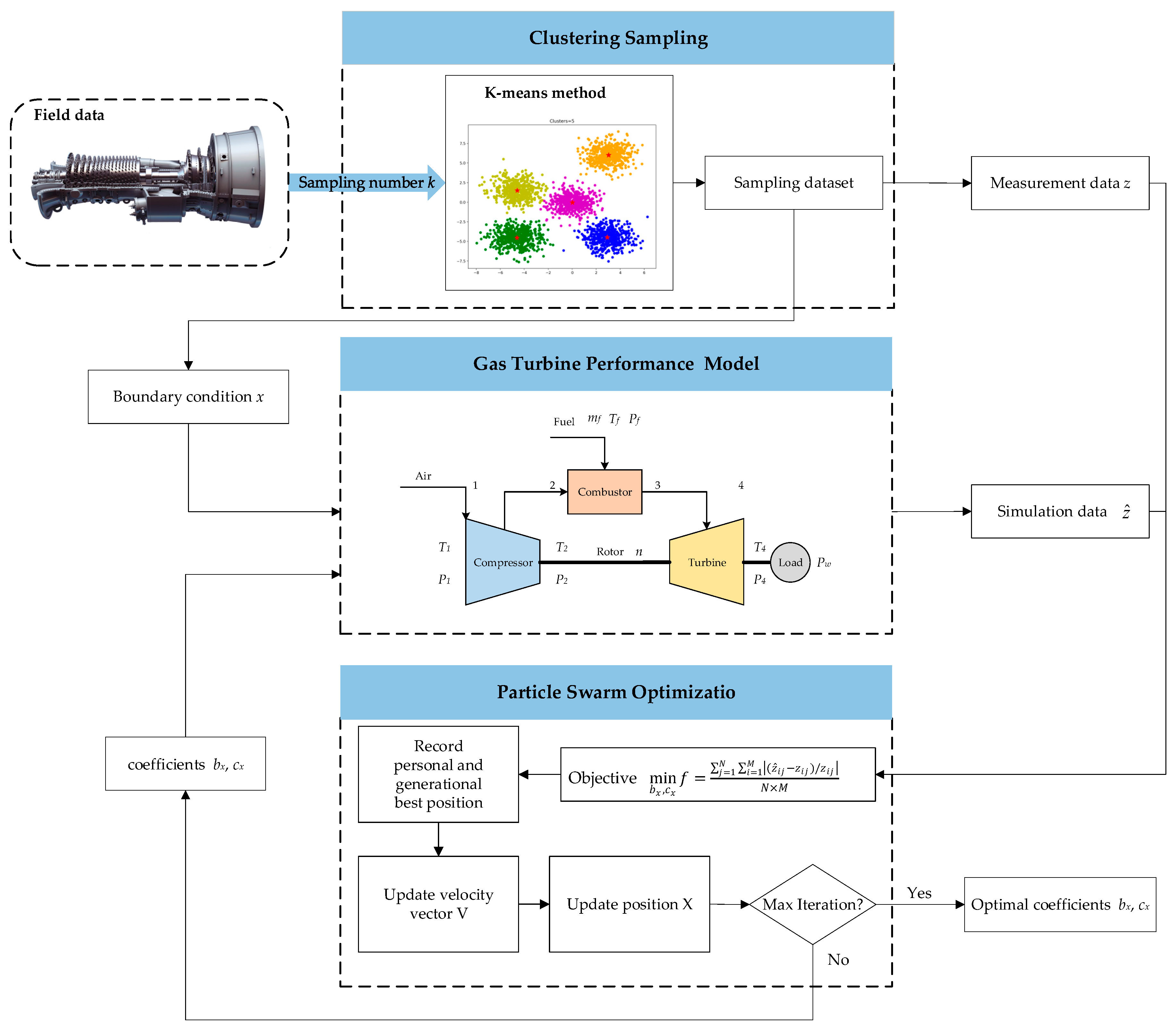
The proposed cluster sampling method divides all operating points into categories and selects the points closest to the cluster centers. Compared with random sampling, it can enhance the coverage and dispersion (representing the degree of sample difference) of the sampling set and enhance the representativeness of the sampling set.

(2)

Compared with the performance model before adaption, the accuracy of the performance model tuned by the particle swarm optimization algorithm (PSO) is increased.

(3)

The proposed method was applied on a real E-class gas turbine power station and compared with the performance adaption based on the random sampling method.

(4)

Compared with the model based on the random sampling method, the proposed method has a higher accuracy in the entire field dataset, especially the overlooked random sampling conditions.

This paper is organized as follows: Section 1 reviews several performance adaptation research and proposes a performance adaption based on cluster sampling and the iteration-eliminating model. Section 2 introduces the simulation model used in this study, performance adaptation, cluster sampling method, and the flowchart of performance adaption based on cluster sampling. Section 3 uses an example of a power plant to demonstrate the effectiveness of the proposed method. Section 4 summarizes this paper.

2. Methodology

The proposed performance adaption process depicted in Figure 1 can tune the component characteristic maps to meet the performance of sampling points extracted from the field data. This method is mainly composed of a gas turbine performance model, a cluster sampling method, and an optimization algorithm. The performance model is described in Section 2.1, the performance adaption method that minimizes the deviation between the field measurement data and the simulated results is described in Section 2.2, the cluster sampling method is described in Section 2.3, and the PSO used to tune the component characteristic maps is described in Section 2.4.

2.1. Performance Model of the Gas Turbine

As performance adaption is conducted on the component-level model, this section introduces the performance simulation model of the gas turbine used in this study. A model consisting of compressor, combustor, turbine, rotator, and generator was used to predict the measurements, as shown in Figure 2. In which, the number “1” means the inlet of compressor, “2” means the outlet of compressor, “3” means the outlet of burner, “4” means the outlet of turbine.

The performance model of the gas turbine was used to simulate the performance parameters with the input parameters. The performance model is a steady-state mechanism model established by thermodynamic principles, energy conservation, mass conservation equations, and the component characteristic maps, which are used to characterize the relationship between the component equivalent flow rate, pressure ratio, isentropic efficiency, and equivalent speed. The simulation model can be expressed as Equation (1):

$$y=f\left(x\right)$$

(1)

where $f(·)$ denotes the mechanism model of the gas turbine; $x=\left\{T_1,P_1,m_f,T_f,P_f,P_4,n\right\}$ is the vector of the input parameters, which are shown by the variables without asterisks in

Table 1. Measurable parameters of the E-class gas turbine.

No.	Measurable Parameters	No.	Measurable Parameters
1	Compressor inlet temperature $T_1$	7	Fuel pressure $P_f$
2	Compressor inlet pressure $P_1$	8	Turbine outlet temperature * $T_4$
3	Compressor outlet temperature * $T_2$	9	Turbine outlet pressure $P_4$
4	Compressor outlet pressure * $P_2$	10	Power output * $P_w$
5	Fuel mass flow $m_f$	11	Rotor speed $n$
6	Fuel temperature $T_f$

* Performance parameters used to test the predicted result.

; and $y=\left\{T_2,P_2,T_4,P_w\right\}$ is the vector of the output parameters, which are shown by the variables marked with asterisks in Table 1.

2.2. Performance Adaption

The gas turbine model was introduced in the previous section, and the component characteristic maps play an important role in the model computation. Therefore, the performance adaption method is proposed to modify component characteristic maps for enhancing the model precision. The basic method of performance adaption used in this paper contains two procedures: (1) Map scaling for design point, which introduces a set of fixed scaling factors to modify the original components’ characteristic maps. This procedure is not described in this paper as it is not its focus. More details can be obtained from Li et al. [17]. (2) Performance adaption for off-design points, in which a set of scaling factors are introduced to improve the prediction accuracy of the simulation model during off-design conditions.

In this paper, the component characteristic maps were adapted according to multiple off-design operation data. As shown in Figure 3, the off-design speed lines in the initial component characteristic map (solid line) are different from the actual map (dotted line). To modify the maps, three characteristic parameters (corrected mass flow rate, pressure ratio, and isentropic efficiency) were calibrated at different speed lines. Taking the compressor as an example, the off-design scaling factors of the corrected mass flow rate, pressure ratio, and isentropic efficiency were introduced and defined as shown in Equations (2)–(4).

It can be observed that the scaling factors at each speed line are different, and the variation of the scaling factors with the speed lines is nonlinear. In this paper, a quadratic form (Equation (5)) was applied to describe the nonlinearity of the corrected relative non-dimensional rotational speed (CN) [17,18].

$$S{F}_{Comp,WAC}=\frac{WA{C}_{Comp,OD}^{\ast }}{WA{C}_{Comp,OD}}$$

(2)

$$S{F}_{Comp,PR}=\frac{P{R}_{Comp,OD}^{\ast }-1}{P{R}_{Comp,OD}-1}$$

(3)

$$S{F}_{Comp,ETA}=\frac{ET{A}_{Comp,OD}^{\ast }}{ET{A}_{Comp, OD}}$$

(4)

$$S{F}_x=1+b_x\left(1-\frac{{\overline{n}}_{OD}}{{\overline{n}}_{DP}}\right)+c_x{\left(1-\frac{{\overline{n}}_{OD}}{{\overline{n}}_{DP}}\right)}^2$$

(5)

In Equations (2)–(4), terms with the superscript “*” mean the modified characteristic parameters and terms without “*” are the original characteristic parameters. The subscript “Comp” means compressor. WAC, PR, and ETA represent the corrected mass flowrate, pressure ratio, and isentropic efficiency, respectively. OD denotes the off-design condition. Equation (5) defines those scaled factors as a quadratic form of CN. x represents one of the characteristic parameters, WAC, PR, and ETA. DP denotes the design point. $b_x$ and $c_x$ represent the first-order and second-order coefficients in the correlation function, respectively. n denotes CN, and $\left(1-\frac{{\overline{n}}_{OD}}{{\overline{n}}_{DP}}\right)$ represents the difference of CN between any OD point and design point.

Figure 3 shows the errors between the original component map and the actual map. The error is larger at a lower speed. Thus, the performance adaption for the off-design points needs to be conducted on the speed lines. During map adaptation, the original map with solid lines were modified to the new map with dotted lines.

Suppose A is a point on a speed line with CN = ${\overline{n}}_{OD}$ with the characteristic parameters PR_A and WAC_A. A* with characteristic parameters PR_A^* and WAC_A^* is the target point at which speed line CN = ${\overline{n}}_{OD}$ should be passed. Let $S{F}_{PR,OD}=\frac{P{R}_A^{\ast }}{P{R}_A}$ and $S{F}_{WAC,OD}=\frac{WA{C}_A^{\ast }}{WA{C}_A}$; after being scaled by Equations (2)–(4), the point A moves to A^* and the speed line with CN = ${\overline{n}}_{OD}$ reaches the dotted line.

In this paper, the scaled factors were decided by CN and the coefficients $b_x$ and $c_x$. CN is an independent input, and $b_x$ and $c_x$ are adjustable parameters. By adjusting the coefficients, the characteristic maps can be modified, and the prediction of the performance measurements changes accordingly. Thus, errors between the actual performance measurements and the predicted performance measurements obtained by the performance model of gas turbine shown in Figure 2 can be minimized by tunning the coefficients $b_x$ and $c_x$.

To obtain the coefficient $b_x$ and $c_x$, the objective function is formed by minimizing the predicted error:

$$\underset{b_x,c_x}{\min }f=\frac{{{\displaystyle \sum }}_{j=1}^N{{\displaystyle \sum }}_{i=1}^M\left|\left({\widehat{z}}_{ij}-z_{ij}\right)/z_{ij}\right|}{N\times M}$$

(6)

where $\widehat{z}$ means the predicted performance measurements, calculated by the simulation model in Figure 2; and $z$ means the actual performance measurements. M represents the number of performance measurements; and N represents the number of targeted off-design points.

2.3. Data Clustering for Sampling

When performing performance adaption, it is inevitable to incur considerable computational cost if all data points are included. It is necessary to select few points from the entire available dataset. The quality of data selection will directly affect the accuracy of the prediction model. The random sampling method can reflect the distribution characteristics of the data to some extent, but it may have difficulties when facing operating condition data. For example, some operating conditions may repeatedly occur in a certain sampling time period, increasing their distribution density. This may easily result in these similar data being sampled multiple times, while some operating conditions are not collected. Thus, a data-clustering technique was employed to learn the intrinsic relationship between data and divide them into different clusters. The basic concept is that similar operating condition data are close to each other and have similar outputs. The clustering technique can help to group points that are within close proximity and find the centroids that have the smallest sum of distances to all other points. In this paper, k-means clustering [26] was used to group the data and find the centroids; then, the data points closest to the centroids were chosen and formed the clustering sampling set to calculate the characteristic adaption. K-means is a representative method of unsupervised learning, which divides data into k classes predetermined according to the distance between the samples. The k-means algorithm has the advantages of fast convergence speed and strong interpretability; its drawback is that the number of k clusters needs to be predetermined, but in this study, it was turned into an advantage as the number of sampling points can be chosen according to the computational needs. On the one hand, cluster sampling can make full use of the collected data. On the other hand, it can also collect data with large feature differences as much as possible. Suppose there are m data points and divide them into k clusters. The calculation steps are as follows:

• Randomly select k points, ${\mu }_1^0$, ${\mu }_2^0$,…, ${\mu }_k^0$, as initial centroids.
• In the t^th iteration step, calculate the distance from each point to the k centroids according to Equation (7), and assign them to the nearest cluster.

  $$distanc{e}_{i,j}^t={\Vert x_i-{\mu }_j^t\Vert }^2, i=1,\dots ,m,j=1,\dots ,k$$

  (7)
• Calculate the mean of the points in each cluster and update the centroids by Equation (8).

  $${\mu }_j^t={{\displaystyle \sum }}_{x_i\in C_j}\frac{x_i}{n}, n is the number of points in C_j$$

  (8)
• Repeat steps 2 and 3, until the difference between two consecutive centroids is smaller than a predefined threshold or the max iteration step is achieved.

2.4. Particle Swarm Optimization (PSO)

Particle swarm optimization (PSO) was used in this study to minimize the function in Equation (6). PSO is a heuristic algorithm proposed by Kennedy and Eberhardt in 1995 [27]. For a detailed description, please refer to Kennedy and Eberhardt [27] and Poli et al. [28]. Each solution of the optimization problem is called a particle. Particles are located in a n-dimension search space with a certain speed, and fitness function is used to evaluate the merits of the particles. The particles can remember and track the personal best position Pbest and global best position Gbest; the speed is calculated according to the flight experience and the best particle position. Suppose the position and velocity of the ith particle at the kth generation is represented as a n-dimension vector:

$$x_{i,k}=\left(x_{i,k}^1, x_{i,k}^2,\dots ,x_{i,k}^n\right)$$

(9)

$$v_{i,k}=\left(v_{i,k}^1, v_{i,k}^2,\dots ,v_{i,k}^n\right)$$

(10)

Then, in the (k + 1)th generation, the position and velocity of particles are updated as follows:

$$v_{i,k+1}=w\times v_{i,k}+c_1\times rand\times \left(Pbes{t}_{i,k}-x_{i,k}\right)+c_2\times rand\times \left(Gbes{t}_k-x_{i,k}\right)$$

(11)

$$x_{i,k+1}=v_{i,k+1}+x_{i,k}$$

(12)

where $Pbes{t}_{i,k}$ represents the previous personal best position of each particle, and $Gbes{t}_k$ refers to the global best position of all particles. rand is a random value from 0 to 1. $c_1$ is the acceleration constant of $Pbest$, $c_2$ is the acceleration constant of $Gbest$, and w refers to inertia weight. The values of w, $c_1$, and $c_2$ can be adjusted depending on the specific problems. In this study, w = 0.5, $c_1$ = 1, $c_2$ = 2, the generation was set to 200, and the population size was set to 20.

3. Results and Discussion

3.1. Application

In this section, the performance adaption method with cluster sampling is applied to a real E-class gas turbine power plant. The gas-path schematic of the gas turbine and the measurable gas-path parameters are shown in Figure 2 and Table 1, respectively. The main parameters in ISO conditions are summarized in

Table 2. Main parameters of the gas turbine power plant in ISO conditions.

Parameters	Value
Output power (MW)	127.6
System efficiency (%)	33.6
Compressor pressure ratio	12.75
Turbine inlet temperature (K)	1397.15
Turbine outlet temperature (K)	821.55

. It was a 127.6 MW gas turbine, with an system efficiency of 33.6%.

The data came from the steady-state operating conditions of the E-class gas turbine from June to November, totally 146 data points. Some measurements of the collected field data are shown in Figure 4. The ranges of the measurements are fuel flow rate $m_f\in \left[14.531 \mathrm{lb}/\mathrm{s}, 16.79 \mathrm{lb}/\mathrm{s}\right]$, compressor inlet temperature $T_1\in \left[294.085 \mathrm{K},315.054 \mathrm{K}\right]$, power output $P_w\in \left[100.717 \mathrm{MW},120.850 \mathrm{MW}\right]$, and turbine outlet temperature $T_4\in \left[832.134 \mathrm{K},849.513 \mathrm{K}\right]$.

3.2. Comparison of Random Sampling and Cluster Sampling

In this section, two sampling methods, cluster sampling and random sampling, are used to select the sampling points for the subsequent performance adaption. The number of sampling data points was set to 10.

Random sampling randomly generates 10 points from the dataset. Cluster sampling uses the k-means clustering algorithm and clusters the 146 data points into 10 clusters based on the variables in Table 1. It produces 10 cluster centers and selects the points closest to the cluster centers as the sampling points. To compare the two sampling methods, the coverage of the total dataset and the coefficient of variation (CV, representing the degree of dispersion) of each sampling set were calculated by Equations (13) and (14), respectively. The analysis results of the two sampling methods are shown in Figure 5:

$$S=\frac{x_{max,sample set}-x_{min,sample set}}{x_{max,total data}-x_{min,total data}}$$

(13)

$$CV=\frac{\sigma }{\mu }$$

(14)

where $x_{max,sample set}$ and $x_{min,sample set}$ are the max and min values of the variables in Table 1 among the selected sample set, respectively; and $x_{max,total data}$ and $x_{min,total data}$ are the max and min values of the variables among the total dataset, respectively. $\sigma$ is the standard deviation of the selected sample set, and $\mu$ is the mean value.

It can be seen that the cluster sampling method can collect data points with large differences as much as possible, which increases the data diversity and extends the coverage of the total dataset. However, using random sampling may lead to repeated sampling and missed sampling.

3.3. Optimization Results

In Section 3.2, two 10-point sampling datasets were formed by using random sampling and cluster sampling. Based on these two sampling sets, the PSO algorithm was used to minimize the performance measurement error by tuning the scaling factor function coefficients. Taking the calculation process of PSO based on cluster sampling as an example, its convergence process is shown in Figure 6.

In which, the red dots represent the iteration steps. It can be seen that the optimization process converges at the 114th generation, where the fitness function is 0.610%. During the optimization process of PSO, the fitness function decreases continuously, indicating that the PSO algorithm significantly reduces the prediction error of the four measurement variables by continuously adjusting the correction coefficients. The average prediction errors of each measurement variable before and after performance adaption are shown in

Table 3. Predicted errors before and after adaption.

Measurements	Before Adaption	After Adaption
Power	3.316%	0.497%
Compressor Outlet Temperature	3.716%	0.316%
Compressor Outlet Pressure	3.359%	0.469%
Turbine Outlet Temperature	1.396%	1.159%
Four Measurements	2.947%	0.610%

. From Table 3, after performance adaption, the accuracy of the performance model was improved, the error of power, compressor outlet temperature, and pressure reached 0.5%, and the error of the turbine outlet temperature reached around 1.1%.

3.4. Comparison of the Prediction Using Random Sampling and Cluster Sampling

In the previous section, the performance adaption processes of two ten-point sampling datasets were completed using the PSO algorithm, and the performance models after adaption based on data points of the random sampling set and the cluster sampling set were obtained, which were denoted as Model 1 and Model 2, respectively. This section compares and discusses the accuracy of these two models using the remaining data points (excluding the sampling points). The prediction errors of the two models based on different sampling methods at the remaining data points are shown in Figure 7.

As can be seen from Figure 7, the cluster sampling correction results are better than the random sampling results in terms of power prediction and compressor outlet pressure prediction. The prediction accuracy of the compressor outlet temperature is similar in both methods, and both are relatively high and around 0.3%; the prediction accuracy of the turbine outlet temperature is also similar in both methods.

Table 4. Predicted errors of the different sampling methods.

Measurements	Error Type	Model 1	Model 2
Power	Average	1.111%	0.552%
	Maximum	2.847%	1.654%
Compressor Outlet Temperature	Average	0.235%	0.249%
	Maximum	0.880%	1.068%
Compressor Outlet Pressure	Average	0.713%	0.411%
	Maximum	2.287%	1.246%
Turbine Outlet Temperature	Average	0.586%	0.650%
	Maximum	3.027%	2.037%
Four Measurements	Average	0.661%	0.466%
	Maximum	1.552%	1.088%

lists the mean error and maximum error of each measured variable in the dataset.

According to Table 4, it can be seen that, overall, the models obtained using random sampling correction and cluster sampling correction have average errors of less than 1.2% for each prediction variable, and the overall average error of cluster sampling is better than that of random sampling. For the power and compressor outlet pressure prediction results, random sampling is slightly worse than the results of cluster sampling, which is reflected in both the average and maximum errors. The average error of power increased by 0.559% and that of the compressor outlet pressure increased by 0.302%. Their maximum errors increased by 1.193% and 1.041%, respectively. For the compressor outlet temperature, the prediction accuracy of both methods is similar, with random sampling results slightly higher than cluster sampling results, but they are generally at the same level of accuracy. For the turbine outlet temperature, the average prediction accuracy is 0.586% for Model 1 and 0.650% for Model 2, basically in the same accuracy level. The maximum error of Model 1 is 3.027%, which can be relatively high, while Model 2 using cluster sampling is 2.037%, improving by 0.685% in comparison with random sampling. In both cases, most prediction errors are below 1.5%, 93.6% for random sampling and 96.0% for cluster sampling. It can be seen that cluster sampling seems to have a certain effect on reducing the maximum error and the average error. This may be due to cluster sampling taking into account multiple clustering conditions and selecting the center points of the conditions, which considers the full range of accuracy and also maintains a certain representativeness for each clustering condition.

To analyze the accuracy improvement created by cluster sampling, the data set was divided into two parts. In Section 3.2, it was mentioned that the k-means algorithm was used to divide the dataset into 10 categories. Cluster sampling selects the points closest to the cluster centers from each cluster to form a sample set, while random sampling picks points directly from the data. Thus, the random sample set may include some clusters and exclude others; so, the data can be classified into two groups: dataset 1, which contains the clusters that were sampled by random sampling, and dataset 2, which contains the clusters that were not sampled by random sampling. Then, the prediction accuracies of the previous Model 1 and Model 2 were evaluated for both groups of data, and the results are shown in

Table 5. Predicted errors of the dataset divided into two parts.

Measurements	Error Type	Dataset 1		Dataset 2
		Model 1	Model 2	Model 1	Model 2
Power	Average	0.938%	0.567%	1.712%	0.501%
	Maximum	2.585%	1.654%	2.847%	1.307%
Compressor Outlet Temperature	Average	0.235%	0.243%	0.235%	0.271%
	Maximum	0.880%	1.068%	0.616%	0.744%
Compressor Outlet Pressure	Average	0.572%	0.392%	1.204%	0.474%
	Maximum	1.731%	1.246%	2.287%	1.041%
Turbine Outlet Temperature	Average	0.432%	0.645%	1.118%	0.670%
	Maximum	2.320%	2.037%	3.028%	1.894%
Four Measurements	Average	0.544%	0.462%	1.067%	0.479%
	Maximum	1.238%	1.088%	1.552%	0.887%

.

By observing columns 1 and 3 of Table 5, it can be seen that the model built using random sampling has some accuracy differences in the two datasets. The model prediction accuracy in the data categories that are not covered by random sampling is lower than that in the data categories that are covered by random sampling. This is reflected in the average and maximum errors of almost all measurement parameters, except the compressor outlet temperature, which is almost the same accuracy level. This result indicates that whether the dataset contains similar operating conditions has a certain impact on the model prediction accuracy, and all operating conditions should be included as much as possible. Observing the prediction results of cluster sampling in the two categories of data, in columns 2 and 4, there is a slight difference but the degree is much lower than that of the random sampling results and almost the same level. This may be because performance adaption is a process of balancing the accuracy of each point, which results in a decrease in accuracy on these categories, or it may be due to some randomness in the results. Observing columns 1 and 2 in Table 5, although both sampling methods cover this part of data categories, and random sampling contains even more data points than cluster sampling, the prediction accuracy does not improve considerably. This may be because cluster sampling not only covers more categories, but also uses the points closest to the cluster center to help to extract the internal features of the data, which can increase the representativeness of the data points. Therefore, more accurate prediction results can be obtained using the cluster sampling method.

Based on Model 2 obtained by the cluster sampling method, the isentropic efficiency of the turbine and energy efficiency were also calculated, and the results are shown in Figure 8. It can be seen that the isentropic efficiency of the turbine was around 88.5% and the system efficiency was around 31.4%.

3.5. Discussion of Random Sampling and Cluster Sampling for a Long Period

To compare and demonstrate the performance of two sampling methods using long-term data, the field data were extended to a one-year period. Figure 9 shows the compressor inlet temperature data in a one-year period. The data were collected every minute and the points with loads below 75% were removed.

Overall, summer is the peak of electricity consumption, and the gas turbine units run for longer periods, resulting in more data points. In contrast, there were less data in winter. The mean value of the compressor inlet temperature was 301.8 K, with a range of [275.9 K, 316.3 K] in a one-year period. The distribution of the dataset is shown in Figure 10.

As can be seen in Figure 10, the data have three distribution centers, corresponding to winter, spring/autumn, and summer. The operation conditions of the field data are naturally over-dispersed due to the over-dispersion of environmental conditions. The field data of high (315 K) or lower (275 K) compressor inlet temperature conditions are much less than that under about 307 K. If the random sampling method is used, theoretically, the distribution of the collected data will be consistent with the original data distribution, mainly distributed around 307 K around summer, and the rest of the data distributed around 294 K and 284 K. This will result in the rare operation conditions being probably covered up by the common operation conditions. Furthermore, considering the computation cost of performance adaption, few sampling points are selected from the original data, making it more likely to miss some operating conditions. Cluster sampling clusters the entire dataset based on the minimum distance to the cluster centers, ensuring the diversity and representativeness of the sampling points. Correspondingly, the clustering method was proposed to detect these rare operation conditions. Taking 10 sampling points as an example, the clustering results and the sampling points obtained by the cluster sampling method are shown in Figure 11, together with random sampling points marked by green triangles.

Compared with the random sampling points, cluster sampling points marked by red circles cover a more diverse range of operating conditions and detect the rare operation conditions both in low and high temperatures. As it can be seen, cluster sampling maintains its advantages of diversity and representativeness even with a longer data collection time and larger data volume.

4. Conclusions

This paper proposed a performance adaption method based on cluster sampling to adjust the component characteristic map and minimize the predicted errors of performance parameters. The tuning factors were the coefficients of scaling factors defined by the ratio of the original and target characteristic parameters. The optimal coefficients were determined by PSO. Through this process, the predicted errors of the performance model can be reduced. Different from other adaption methods, the adaption based on cluster sampling method selects more representative sampling points, which improves the model accuracy on the entire dataset.

The proposed method was applied to a real E-class gas turbine. The simulated performance based on the cluster sampling method was compared with the simulated performance based on the random sampling method. The average and maximum errors of the simulated performance based on the random sampling method on the entire dataset were 0.661% and 1.552%, respectively. The average and maximum errors of the simulated performance based on the cluster sampling method were 0.466% and 1.088%, respectively, all showing some degree of improvement. In the data categories that were not included in the random sample set, the average and maximum errors of the simulated performance based on the random sampling method were 1.067% and 1.552%, respectively. The average and maximum errors of the simulated performance based on the cluster sampling method were 0.479% and 0.887%, respectively. The performance adaption based on cluster sampling enhances the prediction accuracy of the model on the entire dataset and the prediction stability of some operating conditions, and helps to improve the application effect in performance estimation and gas path diagnosis.

Some aspects that can be enhanced in future research are: (1) Clustering is sensitive to outliers in the data. When the data are large, clustering can be used to automatically remove outliers before performing cluster sampling. (2) The current data collection does not include the complete operating data in winter and spring. The model stability on unknown operating conditions can be verified and adjusted in subsequent research.

References

1. Polyzakis, A.L.; Koroneos, C.; Xydis, G. Optimum gas turbine cycle for combined cycle power plant. Energy Convers. Manag. 2008, 49, 551–563. [Google Scholar] [CrossRef]
2. Vyncke-Wilson, D. Advantages of Aeroderivative Gas Turbines: Technical & Operational Considerations on Equipment Selection. In Proceedings of the 20th Symposium of the Industrial Application of Gas Turbines Committee, Banff, AB, Canada, 21–23 October 2013. [Google Scholar]
3. Haglind, F. A Review on the Use of Gas and Steam Turbine Combined Cycles as Prime Movers for Large Ships. Part I: Background and Design. Energy Convers. Manag. 2008, 49, 3458–3467. [Google Scholar] [CrossRef]
4. Tahan, M.; Tsoutsanis, E.; Muhammad, M.; Karim, Z.A. Performance-Based Health Monitoring, Diagnostics and Prognostics for Condition-Based Maintenance of Gas Turbines: A Review. Appl. Energy 2017, 198, 122–144. [Google Scholar] [CrossRef] [Green Version]
5. Li, Y.G. Aero Gas Turbine Flight Performance Estimation Using Engine Gas Path Measurements. J. Propuls. Power 2015, 31, 851–860. [Google Scholar] [CrossRef] [Green Version]
6. Gu, C.; Wang, H.; Ji, X.; Li, X. Development and Application of a Thermodynamic-Cycle Performance Analysis Method of a Three-Shaft Gas Turbine. Energy 2016, 112, 307–321. [Google Scholar] [CrossRef]
7. Tsoutsanis, E.; Meskin, N.; Benammar, M.; Khorasani, K. Transient Gas Turbine Performance Diagnostics through Nonlinear Adaptation of Compressor and Turbine Maps. J. Eng. Gas Turbines Power 2015, 137, 091201. [Google Scholar] [CrossRef]
8. Yang, X.; Guo, X.; Dong, W. On-Line Component Map Adaptive Procedure Based on Sensor Data. In Proceedings of the ASME Turbo Expo 2020, Virtual, 21–25 September 2020. [Google Scholar]
9. Lo Gatto, E.; Li, Y.G.; Pilidis, P. Gas Turbine Off-Design Performance Adaptation Using a Genetic Algorithm; American Society of Mechanical Engineers Digital Collection; ASME: New York, NY, USA, 2008; pp. 551–560. [Google Scholar]
10. Alberto Misté, G.; Benini, E. Turbojet Engine Performance Tuning With a New Map Adaptation Concept. J. Eng. Gas Turbines Power 2014, 136, 071202-1–071202-8. [Google Scholar] [CrossRef]
11. Stamatis, A.; Mathioudakis, K.; Papailiou, K.D. Adaptive simulation of gas turbine performance. ASME J. Eng. Gas Turbines Power 1990, 112, 168–175. [Google Scholar] [CrossRef]
12. Lambiris, B.; Mathioudakis, K.; Stamatis, A.; Papailiou, K. Adaptive modeling of jet engine performance with application to condition monitoring. J. Propuls. Power 1994, 10, 890–896. [Google Scholar] [CrossRef]
13. Kong, C.; Ki, J.; Kang, M. A new scaling method for component maps of gas turbine using system identification. J. Eng. Gas Turbines Power 2003, 125, 979–985. [Google Scholar] [CrossRef]
14. Kong, C.; Kho, S.; Ki, J. Component map generation of a gas turbine using genetic algorithms. J. Eng. Gas Turbines Power 2006, 128, 92–95. [Google Scholar] [CrossRef]
15. Kong, C.; Ki, J. Components map generation of gas turbine engine using genetic algorithms and engine performance deck data. J. Eng. Gas Turbines Power 2007, 129, 312–317. [Google Scholar] [CrossRef]
16. Li, Y.G.; Pilidis, P.; Newby, M.A. An adaptation approach for gas turbine design-point performance simulation. J. Eng. Gas Turbines Power 2006, 128, 789–795. [Google Scholar] [CrossRef]
17. Li, Y.G.; Marinai, L.; Gatto, E.L.; Pachidis, V.; Philidis, P. Multiple-point adaptive performance simulation tuned to aeroengine test-bed data. J. Propuls. Power 2009, 25, 635–641. [Google Scholar] [CrossRef]
18. Li, Y.G.; Ghafir, M.F.; Wang, L.; Singh, R.; Huang, K.; Feng, X. Nonlinear multiple points gas turbine off-design performance adaptation using a genetic algorithm. J. Eng. Gas Turbines Power 2011, 133, 071701-1–071701-9. [Google Scholar] [CrossRef]
19. Li, Y.G.; Ghafir, M.F.; Wang, L.; Singh, R.; Huang, K.; Feng, X.; Zhang, W. Improved multiple point nonlinear genetic algorithm based performance adaptation using least square method. J. Eng. Gas Turbines Power 2012, 134, 031701-1–031701-10. [Google Scholar] [CrossRef]
20. Tsoutsanis, E.; Li, Y.G.; Pilidis, P.; Newby, M. Part-Load Performance of Gas Turbines: Part I—A Novel Compressor Map Generation Approach Suitable for Adaptive Simulation. In Proceedings of the ASME 2012 Gas Turbine India Conference, Mumbai, Maharashtra, India, 1 December 2012. [Google Scholar]
21. Tsoutsanis, E.; Li, Y.G.; Pilidis, P.; Newby, M. Part-Load Performance of Gas Turbines: Part II—Multi-Point Adaptation with Compressor Map Generation and GA Optimization; American Society of Mechanical Engineers Digital Collection; ASME: New York, NY, USA, 2013; pp. 743–751. [Google Scholar]
22. Tsoutsanis, E.; Meskin, N.; Benammar, M.; Khorasani, K. A Component Map Tuning Method for Performance Prediction and Diagnostics of Gas Turbine Compressors. Appl. Energy 2014, 135, 572–585. [Google Scholar] [CrossRef] [Green Version]
23. Yang, Q.; Li, S.; Cao, Y. A New Component Map Generation Method for Gas Turbine Adaptation Performance Simulation. J. Mech. Sci. Technol. 2017, 31, 1947–1957. [Google Scholar] [CrossRef]
24. Li, S.Y.; Li, Z.; Li, S.Y. Improved Method for Gas-Turbine Off-Design Performance Adaptation Based on Field Data. J. Eng. Gas Turbines Power 2020, 142, 041001-1–041001-12. [Google Scholar] [CrossRef]
25. Yan, B.; Hu, M.; Feng, K.; Jiang, Z. Enhanced Component Analytical Solution for Performance Adaptation and Diagnostics of Gas Turbines. Energies 2021, 14, 4356. [Google Scholar] [CrossRef]
26. Hartigan, J.A.; Wong, M.A. Algorithm AS 136: A k-means clustering algorithm. J. R. Stat. Soc. Ser. C Appl. Stat. 1979, 28, 100–108. [Google Scholar] [CrossRef]
27. Kennedy, J.; Eberhart, R. Particle swarm optimization. In Proceedings of the ICNN’95-International Conference on Neural Networks, Perth, WA, Australia, 27 November 1995. [Google Scholar]
28. Poli, R.; Kennedy, J.; Blackwell, T. Particle swarm optimization: An overview. Swarm Intell. 2007, 1, 33–57. [Google Scholar]
Figure 1. Flowchart of the performance adaption method.
Applsci 13 07352 g001
Figure 2. Gas-path schematic of an E-class gas turbine.
Applsci 13 07352 g002
Figure 3. Changes in component characteristic maps in performance adaption.
Applsci 13 07352 g003
Figure 4. The measurements of the E-class gas turbine.
Applsci 13 07352 g004
Figure 5. Sampling coverage fraction and coefficient of the two sampling methods. (a) Sampling coverage fraction of the two sampling methods. (b) Coefficient of variation of the two sampling methods.
Applsci 13 07352 g005
Figure 6. Convergence process based on the clustering sample.
Applsci 13 07352 g006
Figure 7. Comparison of the prediction errors of four different measurements between the two models.
Applsci 13 07352 g007
Figure 8. Prediction of the isentropic efficiency of the turbine and system efficiency.
Applsci 13 07352 g008
Figure 9. The compressor inlet temperature data in a one-year period.
Applsci 13 07352 g009
Figure 10. Data distribution of the compressor inlet temperature.
Applsci 13 07352 g010
Figure 11. Clustering results and sampling points obtained by the two sampling methods.
Applsci 13 07352 g011