Article

Load Forecasting Based on LVMD-DBFCM Load Curve Clustering and the CNN-IVIA-BLSTM Model

1
College of Electric Power, Inner Mongolia University of Technology, Hohhot 010051, China
2
The Sixth Research Institute of China Aerospace Science and Industry Corporation, Hohhot 010010, China
*
Author to whom correspondence should be addressed.
Appl. Sci. 2023, 13(12), 7332; https://doi.org/10.3390/app13127332
Submission received: 27 April 2023 / Revised: 12 June 2023 / Accepted: 15 June 2023 / Published: 20 June 2023
(This article belongs to the Topic Soft Computing)

Abstract

:
Power load forecasting plays an important role in power systems, and the accuracy of load forecasting is of vital importance to power system planning as well as economic efficiency. Power load data are nonsmooth, nonlinear time-series and “noisy” data. Traditional load forecasting has low accuracy and curves not fitting the load variation. It is not well predicted by a single forecasting model. In this paper, we propose a novel model based on the combination of data mining and deep learning to improve the prediction accuracy. First, data preprocessing is performed. Second, identification and correction of anomalous data, normalization of continuous sequences, and one-hot encoding of discrete sequences are performed. The load data are decomposed and denoised using the double decomposition modal (LVMD) strategy, the load curves are clustered using the double weighted fuzzy C-means (DBFCM) algorithm, and the typical curves obtained are used as load patterns. In addition, data feature analysis is performed. A convolutional neural network (CNN) is used to extract data features. A bidirectional long short-term memory (BLSTM) network is used for prediction, in which the number of hidden layer neurons, the number of training epochs, the learning rate, the regularization coefficient, and other relevant parameters in the BLSTM network are optimized using the influenza virus immunity optimization algorithm (IVIA). Finally, the historical data of City H from 1 January 2016 to 31 December 2018, are used for load forecasting. The experimental results show that the novel model based on LVMD-DBFCM load c1urve clustering combined with CNN-IVIA-BLSTM proposed in this paper has an error of only 2% for electric load forecasting.

1. Introduction

As quality of life has improved, the demand for power energy has also risen, and thus, the requirements for power generation and transmission and the use of electricity have increased [1]. Power load forecasting applies machine learning methods to mine the key factors affecting load from historical data, such as weather and time data, to build load forecasting models [2]. Load forecasting is the basis for ensuring the balance of power supply and demand. Accurate forecasting results can reduce the pressure on transmission and distribution links and facilitate the optimal scheduling of power transmission links. They can effectively reduce power generation costs and improve economic and social benefits [3,4].
Traditional forecasting methods use the overall historical load numbers as their basis [5,6,7,8,9]. The trend extrapolation predicts future loads based on the historical trends of the predictor variables. It predicts near future loads with high accuracy, but error gradually increases with time. The regression analysis method predicts future load changes by establishing a functional relationship between variables. It has high fitting ability but has a large error in predicting future changes. Time series extrapolation (the autoregressive moving average model) approximates a nonlinear relationship with a linear equation [10]. The grey forecasting method performs correlation analysis by identifying the degree of dissimilarity in development trends between system factors. Traditional forecasting models have a relatively simple structure and require highly accurate historical data, resulting in forecasting results with poor accuracy.
In recent decades, deep learning has made important breakthroughs in the field of artificial intelligence. In 1957, Frank Rosenblatt invented an artificial neural network to solve complex problems by means of a multilayer perceptron (MLP). Deep neural networks (DNNs) are currently a popular topic in load prediction research, and recurrent neural networks (RNNs) have advantages in memory parameter sharing and Turing completeness [11]. Long short-term memory (LSTM) networks overcome the problem that RNNs are prone to gradient disappearance/explosion, but their ability to correct errors is weak [12]. M. Schuster proposed a BLSTM network that can make full use of the hidden layer history state and has stronger robustness [13]. Yet, BLSTM networks have many parameters, and without proper optimization, the model may be overfitted or slow to train, resulting in inefficiency. The number of hidden layer neurons, the number of training epochs, the learning rate, and the regularization coefficient in the BLSTM network are optimized using the IVIA. It can improve the model’s efficiency. The challenges of the machine learning algorithms to load forecasting for power systems, with complex, nonsmooth, nonlinear time-series and “noisy” data, will decrease the accuracy of the algorithm, and a single prediction model has difficulty meeting the accuracy requirements. Integrating a hybrid preprocessing method can significantly improve the prediction accuracy [14,15,16,17].
In summary, to improve the accuracy and meet the needs of practical problems, this paper proposes a new model based on data mining and deep learning. It considers not only historical load data but also weather information, date types, real-time electricity prices, etc. Historical data load, weather information, and real-time electricity prices are normalized, and the date and holiday information are expressed through One-Hot encoding. The DBFCM algorithm is applied to load curve clustering to overcome the problems of traditional C-means clustering and fuzzy C-means clustering in which data are clustered into small classes, inaccurate classification is performed, and the “uniform effect of the cluster size” degrades performance. First, the LVMD is used to decompose and denoise the input data to improve the continuity and stability of the data. Second, the DBFCM algorithm is used to perform load curve clustering. Third, feature fusion extraction is performed using CNN. In addition, the extracted feature vectors are used as the input of IVIA-BLSTM. The IVIA is proposed to optimize the parameters in the BLSTM network. Finally, this paper proposes a new load forecasting model based on the LVMD-DBFCM algorithm and CNN-IVIA-BLSTM.
The remainder of this article is organized as follows. Section 2 describes the IVIA algorithm, Section 3 presents the methodology used in this paper, Section 4 is a case study of this paper, and Section 5 concludes the paper.

2. Influenza Virus Immunity Optimization Algorithm

The IVIA is a new metaheuristic optimization algorithm that is inspired by the way influenza viruses spread in a population and the process of population immunity. The process of an individual being infected is divided into three states: uninfected, infected, and immune, and the population has herd immunity when the number of immune individuals in the population exceeds 80% of the total population. This section examines the IVIA with 23 sets of standard test functions and compares it with seven optimization algorithms proposed in recent years. They are turbulent flow of water-based optimization (TFWO) [18], golden eagle optimization (GEO) [19], the parasitism–predation algorithm (PPA) [20], the rat swarm optimizer (RSO) [21], gray wolf optimization (GWO) [22], particle swarm optimization (PSO) [23], and whale optimization algorithm (WOA) [24]. The results of the tested functions show that the IVIA converges faster with higher accuracy, optimizes the function better, and finds the optimal value of the function in fewer iterations. Then, the IVIA is applied to the neural network BLSTM training of the power load forecasting model to optimize the number of hidden layer neurons, the number of training epochs, the learning rate and the regularization coefficient, and other relevant parameters to improve the accuracy of the forecasting model.

2.1. Biological Characteristics

The influenza virus is very contagious, spreads quickly, and has many routes of transmission [25]. The spread of the virus in the population can be achieved through droplet transmission and physical contact, and the rate of spread is related to the social distance between people [26]. The vast majority of the population can recover on their own after infection, and those who recover produce the corresponding antibodies in their bodies and have immune functions. A small number of people with underlying diseases, that is, elderly people or those with weak resistance, are at risk. When the number of immune individuals in the population exceeds 80%, the population has herd immunity, thus preventing the next round of disease transmission. A schematic diagram of the transmission process of the influenza virus in a population is shown in Figure 1.
The population is divided into infected individuals, highly susceptible individuals, susceptible individuals, safe individuals, and absolutely safe individuals.
Extremely susceptible individuals are direct contacts of infected individuals, who are socially close to infected individuals and are infected by getting influenza virus from infected individuals; susceptible individuals are indirect contacts of infected individuals who are socially distant from the infected individuals, may be infected through third parties as vectors, and have a higher risk of infection; safe individuals are not in contact with infected individuals or other individuals, and because the influenza virus is transmitted as a vector, through a change in social distance, safe individuals may become susceptible individuals or infected individuals; absolutely safe individuals have immune functions through vaccination or healing after infection and are not susceptible to infection, regardless of the contact distance of infected individuals. In this paper, the influenza virus immunization algorithm is proposed through the transmission of the influenza virus in a population and the immunization mechanism. To map the spread process of the influenza virus with the optimization algorithm, the following assumptions are made:
  • The initial number of infected individuals is small, and they are randomly distributed in the population. The category to which an individual currently belongs and the corresponding update formula are determined based on the distance between the individual and the infected individual;
  • The overall number of the population is kept constant, and absolutely safe individuals randomly move to different locations in the population. The number and location of other individuals change dynamically with the number of iterations;
  • Individuals in the population have three states: infected, uninfected, and immune. Infected individuals have immunity after infecting other individuals and will not be infected in the following process. A population is immune when 80% or more of the individuals in the population are immune;
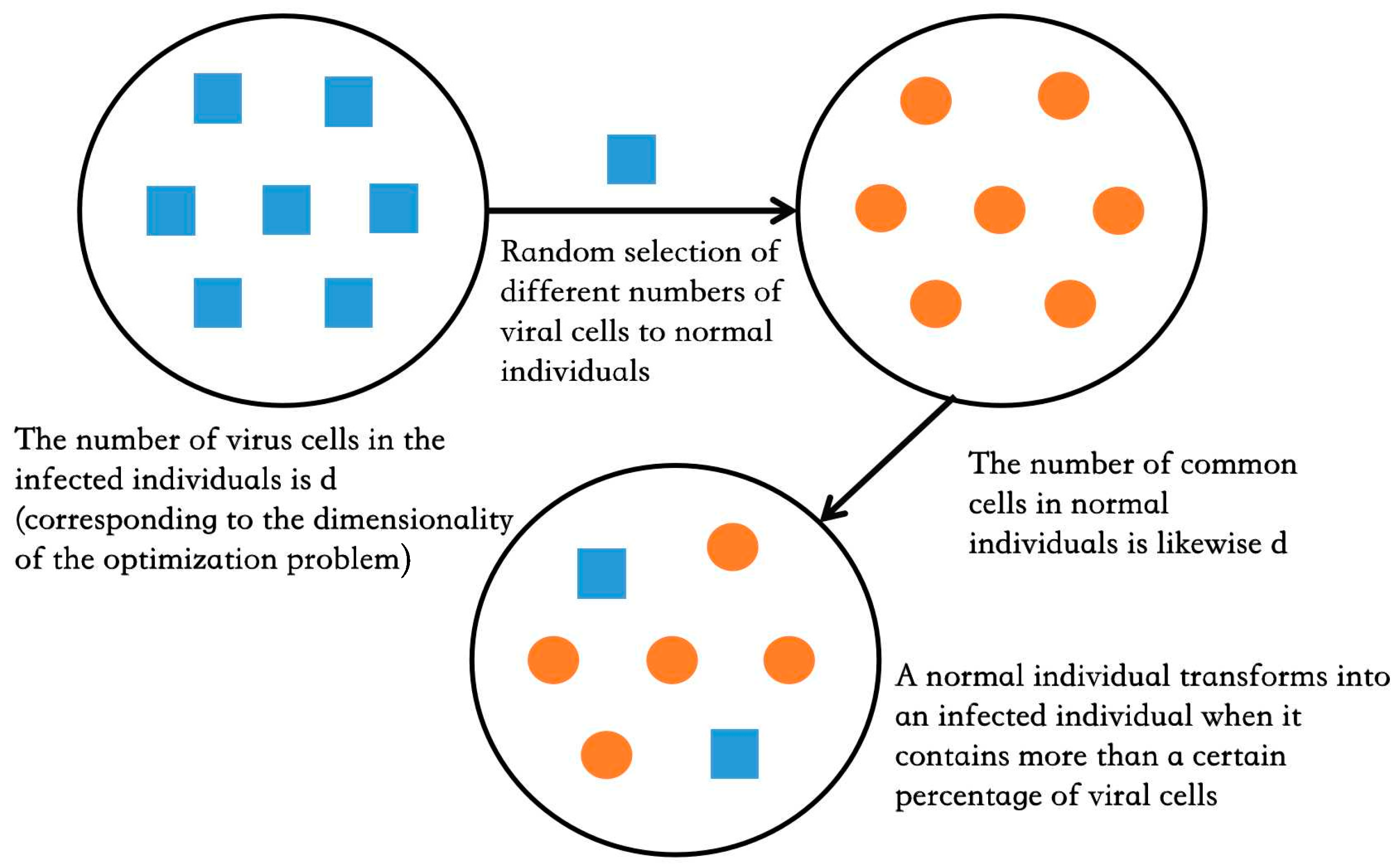
  • Individuals are infected by contracting virus cells from an infected person, and the process of virus cell exchange is shown in Figure 2. The influenza virus cells and the diseased cells are taken as the smallest units within an individual to represent the dimension of the optimization problem.
Immunized individuals: The individuals who are categorized as immunized are protected against the virus, and they are not affected by infected individuals.
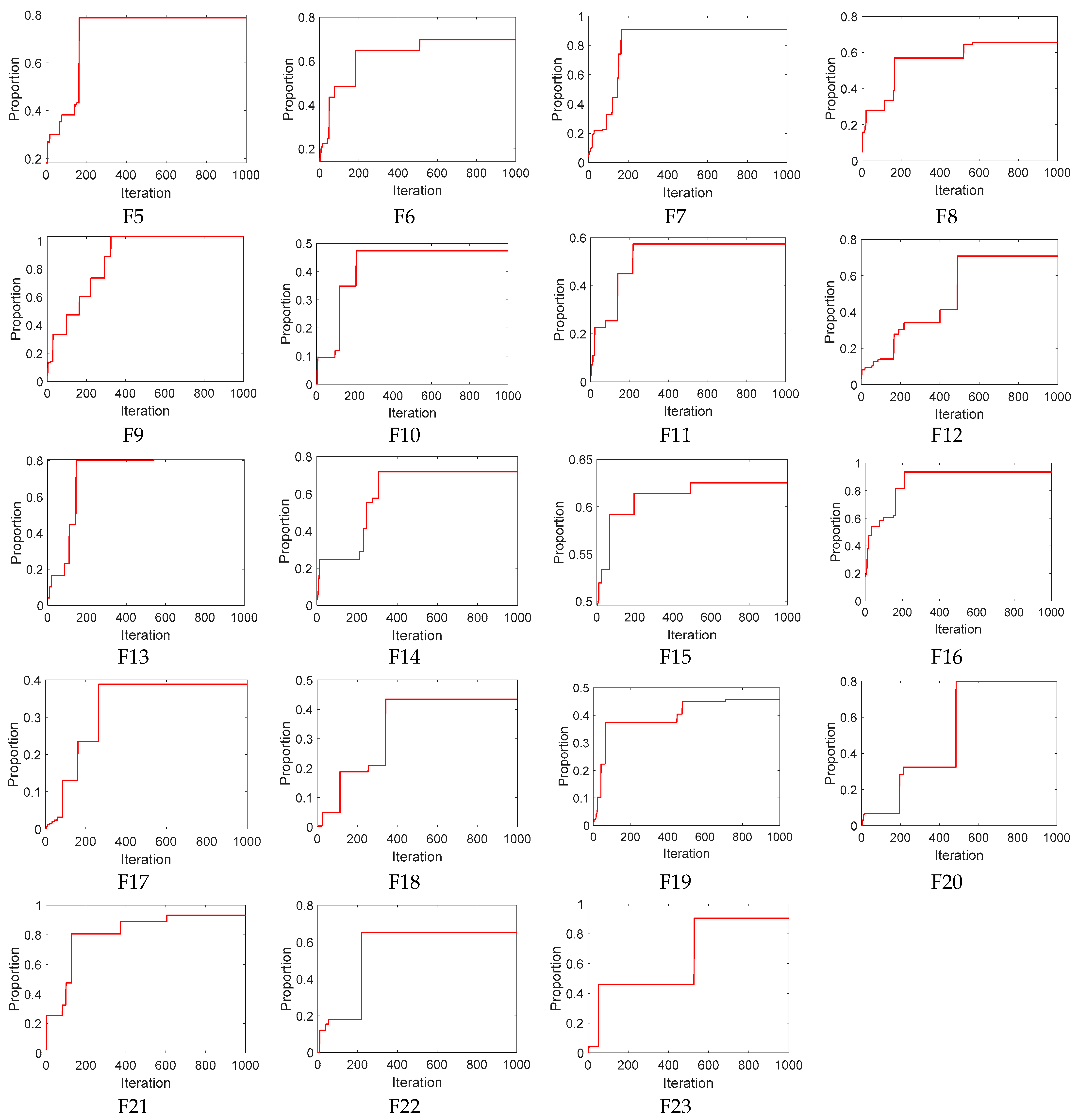
Figure 3 shows the proportion of immune individuals to the entire population with the 23 sets of standard test functions run by IVIA. From the figure, except for functions F4, F7, F9, F16, F21, and F23, all the remaining 17 tested functions stop the iterative search process when the population immunity rate reaches 0.8. In this paper, the minimum population immunity rate for IVIA is set at 0.8, i.e., the search for optimization stops when the number of immunized individuals in the population exceeds 80% of the total. It ensures that the algorithm has high optimization results.
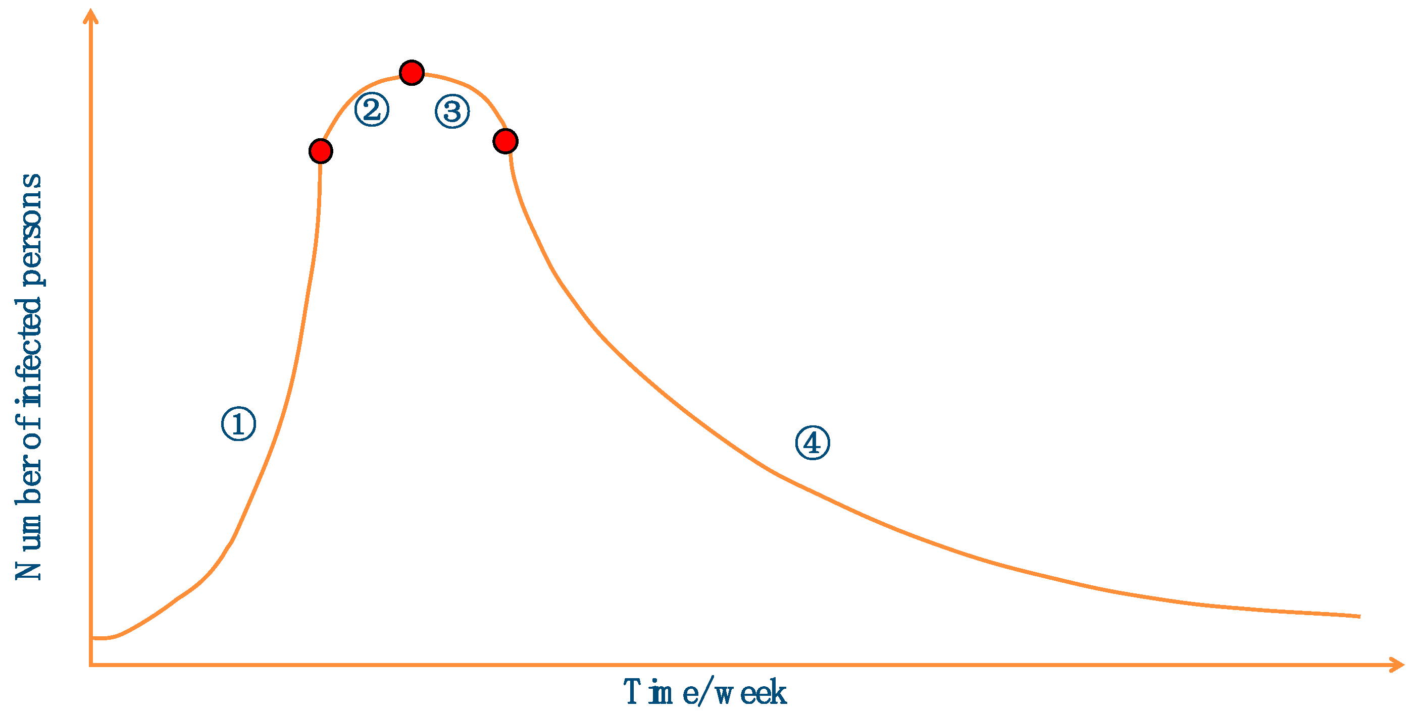
In this paper, we propose the IVIA based on the transmission and immunization process of the influenza virus. The influenza virus spreads rapidly in a population, and the growth curve of the cumulative number of infections is shown in Figure 4. Curve ① indicates that the number of infected individuals in the population increases rapidly within 2~3 weeks, and curves ② and ③ indicate that the number of infected individuals peaks at 7~8 weeks and then gradually starts to decline. Curve ④ indicates that the number of infected individuals gradually decreases and the number of immunized individuals increases near the end of this influenza outbreak. The IVIA has a good optimization capability at the beginning of the iteration. Figure 4 is a schematic diagram summarized according to the epidemic transmission rules; the website of the epidemic transmission rules is shown below.

2.2. Mathematical Model

The process of influenza virus transmission in a population is mapped with the influenza virus immunization algorithm. The population is represented by the matrix X , as shown in Equation (1), where n is the population size and the number of individuals, and d is the number of cells invaded by the influenza virus into the human body, corresponding to the dimensionality of the objective function. The initialization process of the algorithm randomly generates an n × d dimension matrix X , which sets the initial number of infected individuals to x .
X = [ x 11 x 12 x 1 d x 21 x 22 x 2 d x n 1 x n 2 x n d ]
The fitness values of different individuals in the population are represented by Equation (2). Each row in the matrix is represented as the fitness value of the current individual. The individual corresponding to the optimal fitness value is the current optimal solution of the objective function.
F ( x ) = f ( x 11 ,   x 12 , ,   x 1 d ) f ( x 21 ,   x 22 , ,   x 2 d ) f ( x n 1 ,   x n 2 , ,   x n d )
The distance between individuals is represented by C, as shown in Equation (3). x = { x 1 ,   x 2 ,   ,   x d } is the position of individual x, y = { y 1 ,   y 2 , ,   y d } is the position of individual y, and d is the dimension of the optimization problem.
C = ( x 1 y 1 ) 2 + ( x 2 y 2 ) 2 + + ( x d y d ) 2
L is the maximum safety distance, as shown in Equation (4). ( L min ,   L max ) represents the range of values for individuals.
L = 1 2 L min 2 + L max 2
The virus spreading process corresponds to the iterative optimization-seeking process in the algorithm. It is assumed that the safe distance between other individuals and the infected person when the influenza virus spreads in the population is L. The iterative formulas for individuals in different cases are shown in Equations (5) to (9).
  • Infected individuals are updated by Equation (5):
x i , j ( t + 1 ) = x i , j ( t ) exp N max n N max 1 × 1 d 1 q
When the contact distance between individuals in the population and infected individuals is C < 0.2 L , the individuals are moved into the infected state. The position of infected individuals is updated by Equation (5). N max is the maximum number of iterations, n is the current number of iterations, d is the dimensionality of the optimization problem, and q is used to regulate the individual position update rate. The larger the value is of q , the faster the position update rate and the higher the accuracy of the optimization search.
  • Extremely susceptible individuals are updated by Equation (6):
x i , j ( t + 1 ) = x i , j ( t ) + α x i , j ( t ) x i , q ( t ) α = 1 d p = 1 d r a n d ( 1 , 1 )
When the contact distance between individuals in the population and infected individuals is 0.2 L < C < 0.5 L , the position is updated by Equation (6). x i , q ( t ) is the random acquisition of viral cells by highly susceptible individuals; α represents update coefficient at the contact distance of 0.2 L < C < 0.5 L . When the number of exchanged cells exceeds a quarter of the total number of cells, the highly susceptible individuals are transformed into infected individuals. Cell exchange occurs only once during each iteration, and the number of exchanges is random.
  • Susceptible individuals are updated by Equation (7):
x i , j ( t + 1 ) = x i , j ( t ) + β x i , j ( t ) x i , v ( t ) β = exp C L ε × N max ε = r a n d ( 0 , 1 )
When the contact distance between individuals in the population and infected individuals is 0.5 L < C < 0.8 L , the position is updated by Equation (7). x i , v ( t ) is a random acquisition of viral cells by highly susceptible individuals, β represents update coefficient at the contact distance of 0.5 L < C < 0.8 L , ε is a random number in the range 0~1. When the number of exchanged cells has exceeded one-third of the total number of cells, the highly susceptible individuals are transformed into infected individuals.
  • Secure individuals updated by Equation (8):
x i , j ( t + 1 ) = x i , j ( t ) + γ x i , j ( t ) x i , w ( t ) f ( x i , w ) = arg min f ( x i , j ) γ = r a n d ( 1 , 1 )
When the contact distance between individuals in the population and infected individuals is 0.8 L < C < L , the position is updated by Equation (8). γ is a random number in the range −1~1. There is no cellular exchange between safe individuals and infected individuals. However, as the number of infected individuals increases, the contact distance between safe individuals and infected individuals may decrease, and safe individuals may become susceptible.
  • Absolutely safe individuals updated by Equation (9):
x i , j ( t + 1 ) = λ x i , j ( t ) λ = γ × 2 1 2 L
Absolutely safe individuals are immune, and the contact distance between individuals and infected individuals is C > L ; λ represents the update coefficient at the contact distance of C > L . They randomly change their positions during the iterative process and can be used to escape the current search region when the algorithm falls into local optima.
Stop criterion IVIA: The algorithm terminates when the number of immune individuals in the population exceeds more than 80% of the population or when the maximum number of iterations is reached. Therefore, the individual with the highest population immunity corresponds to the optimal solution of the optimization problem, and the corresponding function value is the optimal value of the optimization problem. If the problem to be solved requires higher accuracy, the population immunity rate in the Algorithm 1 can be increased. The pseudo-code of IVIA is presented below.
Algorithm 1 IVIA pseudo-code
Input:
n: The number of people
Nmax: The maximum number of iterations
m: Initial number of infected individuals (usually set to 1)
L: Maximum safe contact distance
R: Herd immunity ratio
C: The distance between individuals
lb,ub: Search boundary
1: Population initialization
2: Setting parameters
3: while (t < N)
4:        Calculate fitness value and sort
5:      for i = 1:n
6:          if (C < 0.2L) then
7:             Using Equation (5) to update the location of the infected individuals
8:             Record the current status of the individuals
9:          else if (0.2L < C < 0.5L) then
10:           Using Equation (6) to update the location of highly susceptible individuals
11:           Record the current status of the individuals
12:        else if (0.5L < C < 0.8L) then
13:           Using Equation (7) to update the location of susceptible individuals
14:           Record the current status of the individuals
15:        else if (0.8L < C < L) then
16:           Using Formula (8) to update the position of a safe individuals
17:           Record the current status of the individual
18:        else
19:           Using Equation (9) to update the position of an absolutely safe individuals
20:        end if
21:        Recalculate fitness value
22:    end for
23:    Calculate immunity rate
24:    t = t + 1
25: end while

2.3. Algorithm Testing

To test the actual optimization effect of the proposed IVIA, it was evaluated in this paper on 23 sets of standard test functions. The optimization results were compared with those of turbulent flow of water-based optimization (TFWO), golden eagle optimization (GEO), the parasitism–predation algorithm (PPA), the rat swarm optimizer (RSO), gray wolf optimization (GWO), particle swarm optimization (PSO), and the whale optimization algorithm (WOA).
Table 1 shows the expression of the test function, the dimension of the optimization problem, and the overall search range, and the last column shows the minimum value of the test function expectation, which is the theoretical optimum. The IVIA population size n is 30, the maximum number of iterations N max is 1000, the maximum safe contact distance L is 0.5 u b , and the population immunity rate R is 80% during the test period. The number of dimensions of the test function and the parameters, such as search intervals l b and u b , are set according to Table 1. The overall and iteration numbers of the other optimization functions are the same as those of the IVIA.
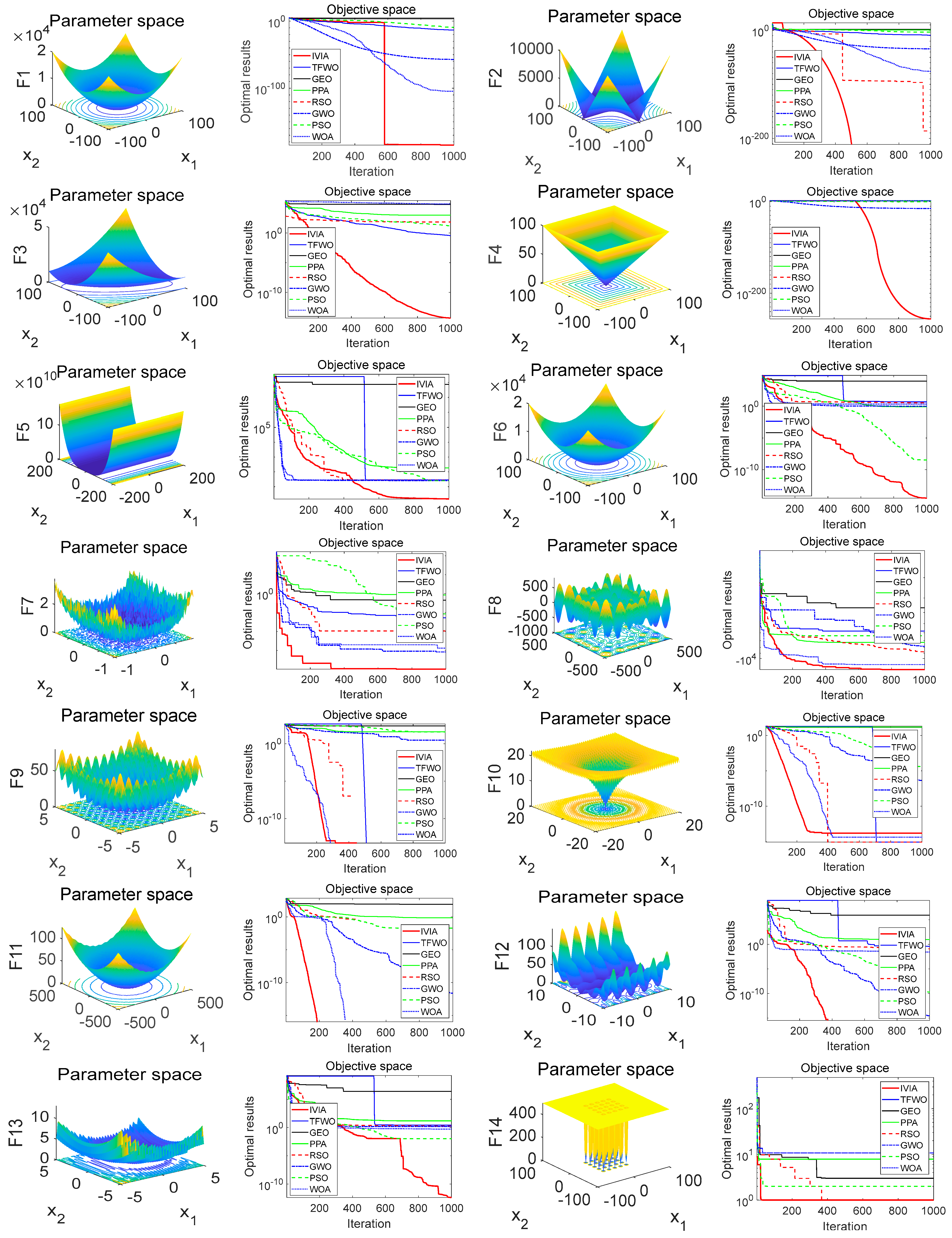
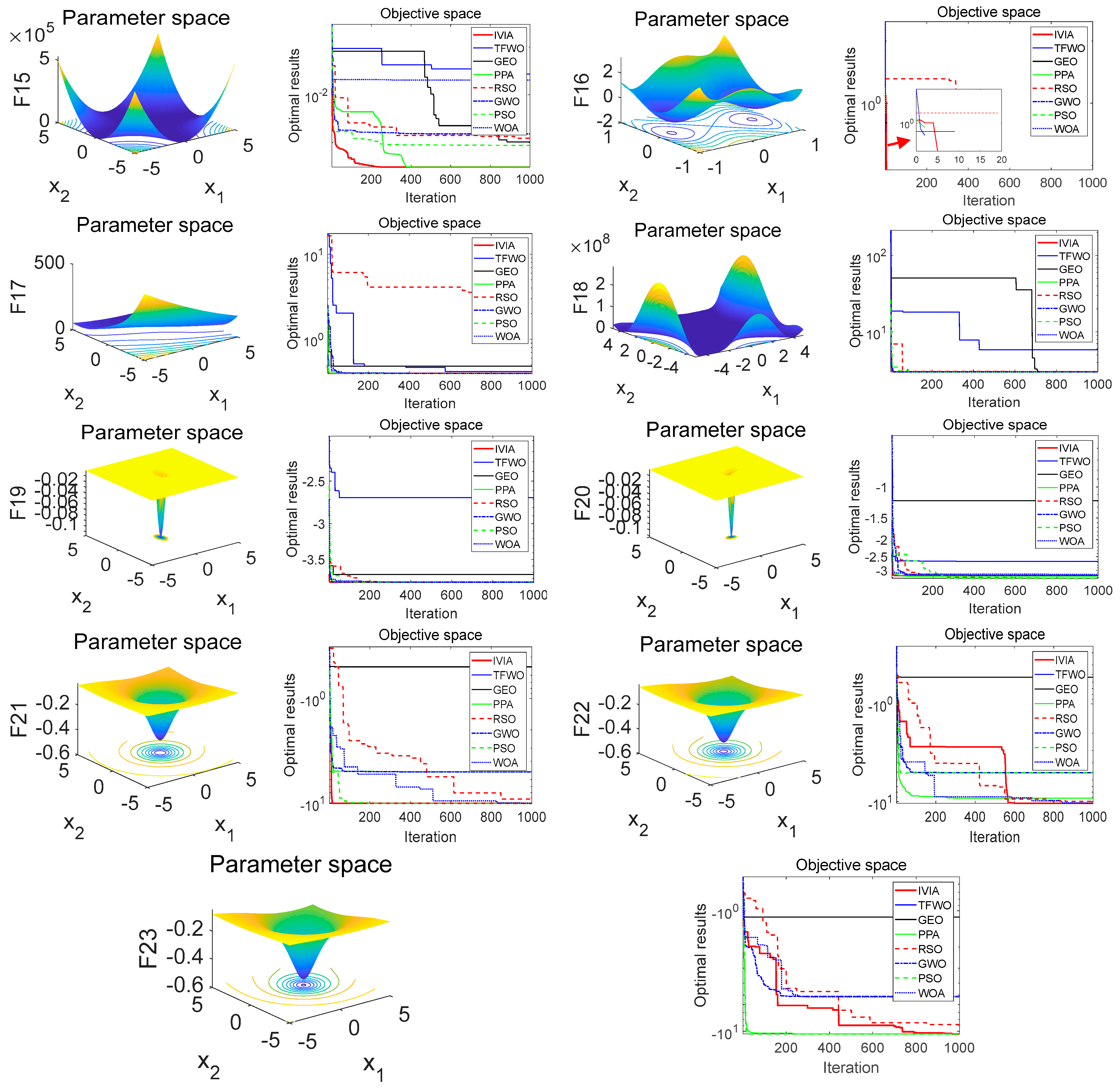
The viability of the proposed IVIA is tested using 23 well-known benchmark functions with different sizes and complexity. Figure 5 shows the three-dimensional graphs of the standard test functions and their corresponding test results. The convergence of the IVIA is very good for both single-peaked and multipeaked functions.
From the test results in Table 2, the accuracy of the IVIA for function finding is much higher than that of several other optimization algorithms, and the theoretical optimal value can be found for some functions. IVIA has fewer iterations, a shorter running time, and faster convergence compared to the other seven algorithms.
For comparative evaluation, the proposed IVIA is compared against seven well-established comparative methods using the same benchmark functions. IVIA optimizes best in F1, F2, F3, F4, F5, F6, F7, F8, converges fastest in F11, F12, F13, F14, F15, F17, and it has the same effect as other algorithms in F18, F19, F20, F21, F22, F23. The comparative results show the effectiveness of IVIA.
In summary, the IVIA is based on the characteristics of fast convergence, better robustness, and good optimization search. In this paper, the IVIA is selected to optimize the relevant parameters, such as the number of neurons in the hidden layer, the number of training times, the learning rate, and the regularization coefficients in the BLSTM network.

3. Methodology

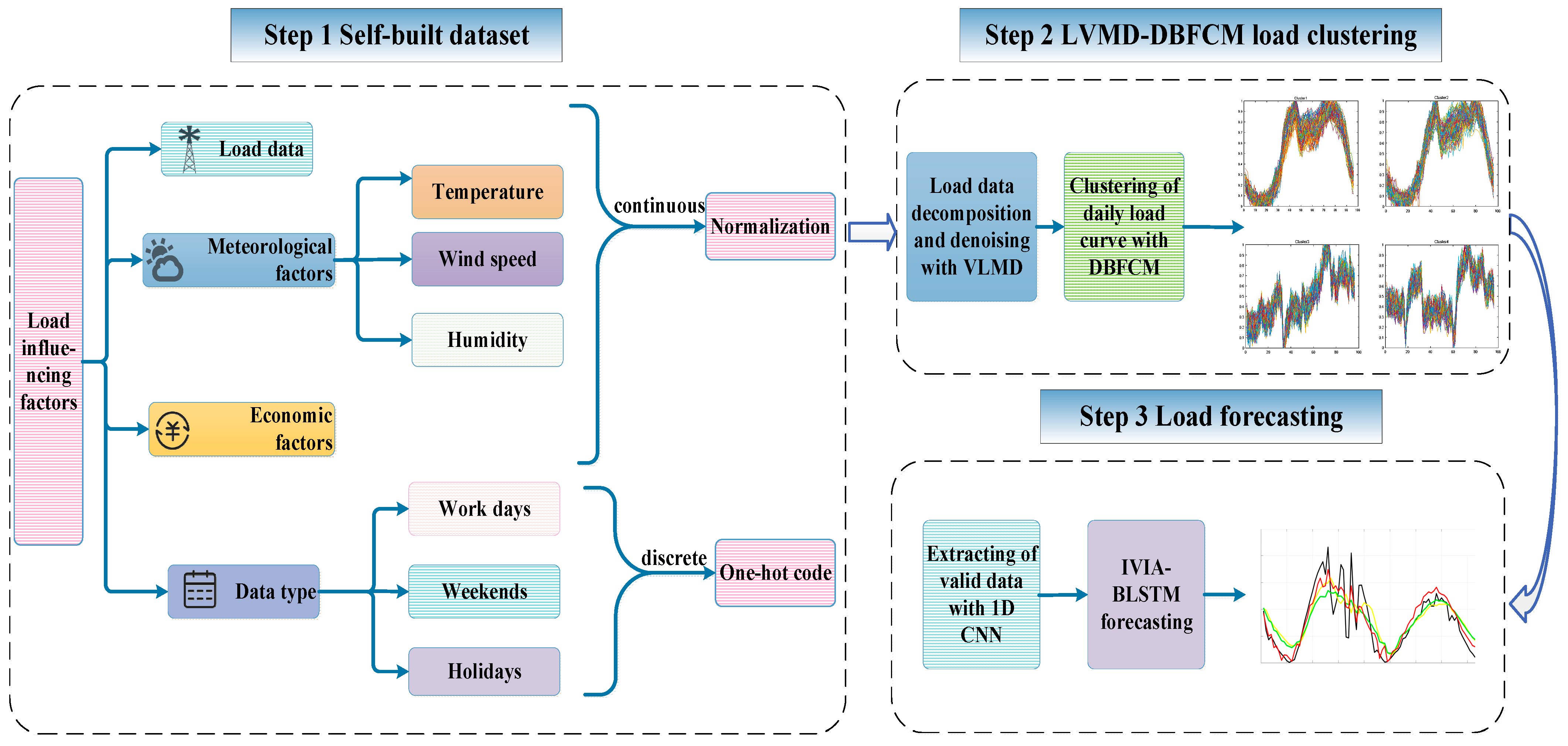
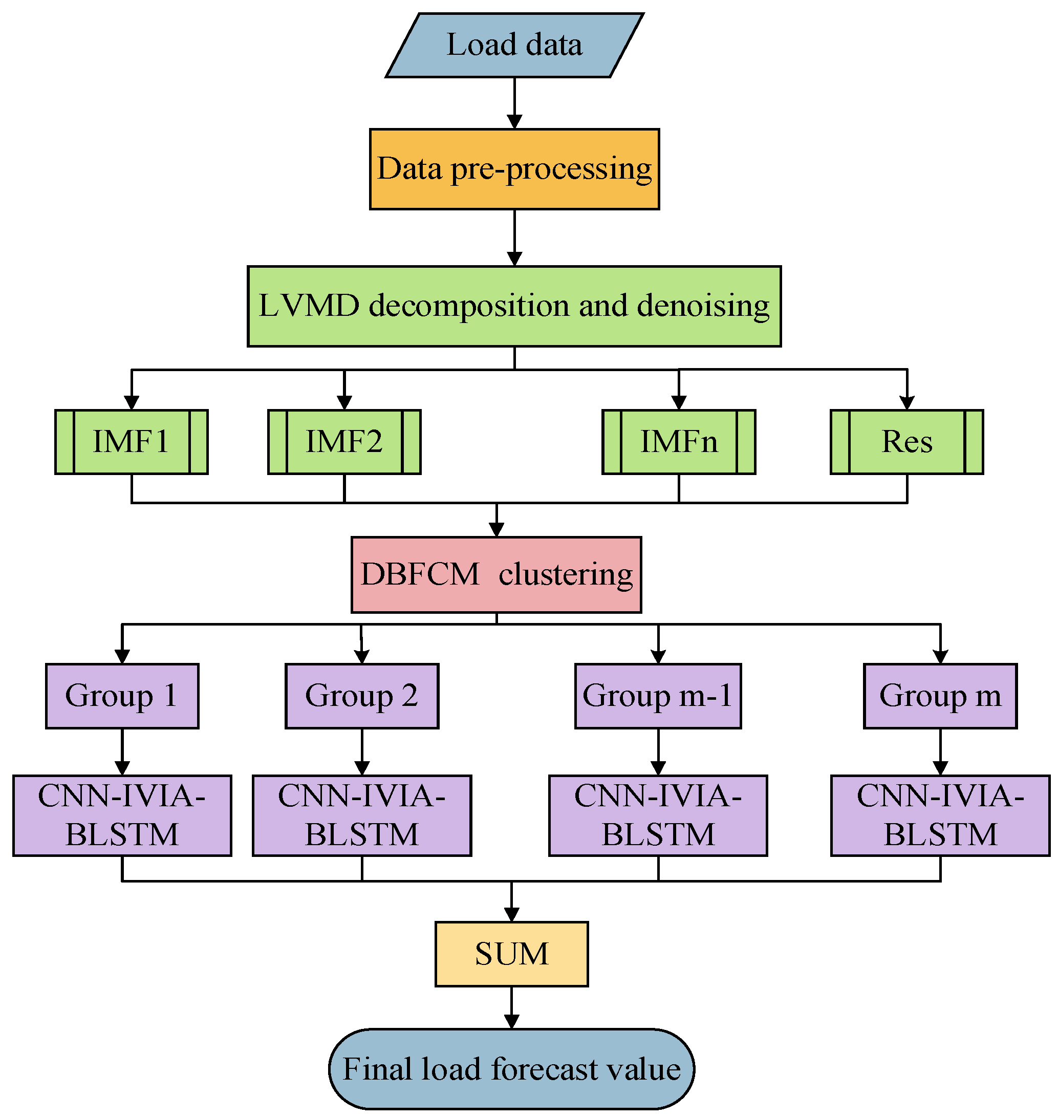
In this paper, we propose a method for power load forecasting based on LVMD-DBFCM load curve clustering, and the CNN-IVIA-BLSTM model is shown in Figure 6. First, data preprocessing is performed, and the influences of load are divided into continuous and discrete series. After normalizing the continuous sequences, they include load data, meteorological data (temperature, wind speed, and humidity), and economic factors. One-hot encoding is applied to discrete sequences, and the discrete sequences include the data types of workdays, weekends, and holidays. Load data decomposition and denoising with LVMD are performed on the preprocessed data. Then, the power load curve is clustered using the DBFCM algorithm. The processed data are extracted with a 1D CNN for feature extraction and finally, predicted with the IVIA-BLSTM model.

3.1. Self-Built Dataset

We expect to study the electrical load of a particular city or region where such datasets are rare. Data from the internet are collected and organized to produce an HS dataset. The following cities are replaced by H City because the electricity data relate to the economic performance of the country. The dataset includes 1096 days of electricity load data from 1 January 2016 to 31 December 2018, in H City. The dataset was divided; 80% is used as the training set and 20% is used as the test set.
The effects of the three factors of temperature, humidity, and wind speed on the power load are as follows. In summer, the temperature is high, and as air-conditioners usage increases, the power load increases. When the relative humidity is in the sensitive range 40~95%, the meteorological sensitive load varies significantly with the relative humidity. The load decreases with the increase of relative humidity. When the wind speed is in the sensitive range 2~6 m/s, the weather sensitive load changes significantly with the wind speed. The load increases with the increase of wind speed [27].

3.1.1. Dataset Visualization

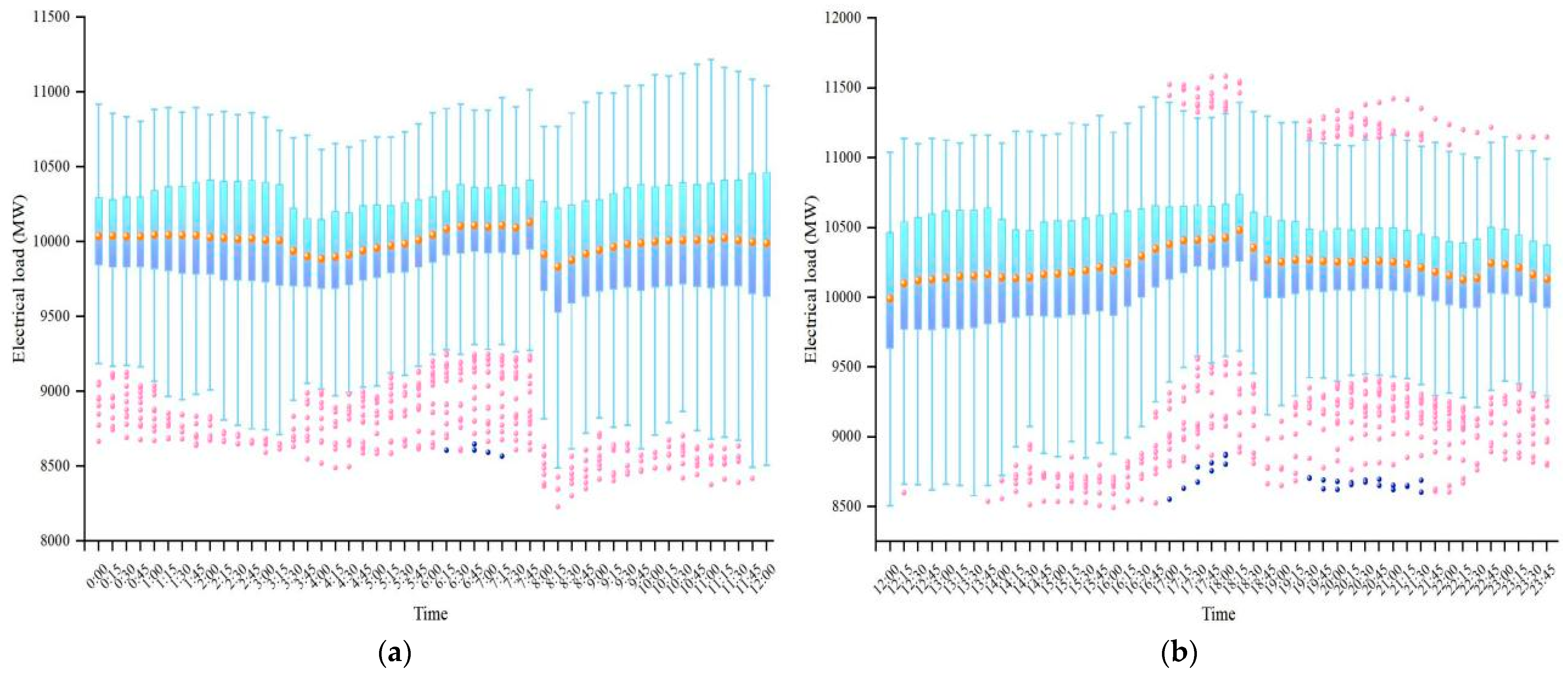
The overall power load data from 2016–2018 are presented in Figure 7. From the box-whisker plot, the difficulty of prediction is reflected by the high number of data outliers in the morning from 6:00 to 8:00 and in the afternoon from 17:00 to 18:00 and 19:45 to 22:00. In summary, the importance of the data preprocessing and clustering and prediction models that follow in this paper is illustrated.

3.1.2. Data Preprocessing

  • Abnormal data recognition and correction
Data preprocessing is first performed to resolve data outliers before clustering and prediction is performed [28].
Missing data: Lagrange interpolation is used to handle missing values.
Data duplication: Remove duplicate datasets by similarity.
Data mutation: 3 criteria.
  • Data normalization
Normalized values for the clustering process can reduce the adverse effect on the clustering effect in the data domain due to the weight of the distance occupied between different attributes of the initial values. Normalization can eliminate the influence of the size of the load data volume on the distance in the clustering analysis, and thus, the information on the load pattern is highlighted [29].
Data normalization: Uniform metrics on data. Z Score normalization is shown in Equation (10). After normalization, the load data are normalized to the interval [−1, 1].
Z X = x i X ¯ σ
Data preprocessing: The equation for normalizing continuous data is given in Equation (11). Using One Hot encoding for discrete sequences, each state has unique register bits; only one bit is 1, and the rest are 0.
M i n M a x x = x i x min x max x min

3.2. LVMD-DBFCM Imbalanced Data Clustering

The goal of load clustering is to mine the typical daily load model [30].
Step 1. De-noising. The load data are decomposed and denoised using the LVMD (in Section 3.2.1).
Step 2. Clustering. The load data are clustered using the DBFCM (in Section 3.2.2).
Step 3. Clustering evaluation. The load data clustering effect are analyzed using the SSE evaluation index (in Section 3.2.3).

3.2.1. LVMD Double Decomposition Modal Strategy

  • VMD Variational Mode Decomposition
VMD [31] is an iterative process that is used to search for the optimal solution of a variational model and to determine the mode u k ( t ) and its corresponding central frequency w k and bandwidth. VMD has good denoising capabilities. VMD denoising are as follows:
  • Initialize parameters u ^ k 1 , w k 1 , λ ^ 1 , and let n = 0 .
  • n = n + 1 , update w k and u k .
  • k = k + 1 , repeat the previous step until k = K .
  • Update λ , and the equation is shown in Equation (12).
  • Repeat steps 2–5 until the end, when the condition of Equation (13) is satisfied.
  • The component that contains the minimum time information after decomposition is judged and considered to be random noise that is eliminated. Then, the data are reconstructed by the remaining modal component pairs, and the reconstructed data are the load data that do not contain noise.
λ ^ n + 1 ω = λ ^ n ω + τ f ^ ( ω ) k u ^ k n + 1 ( ω )
k u ^ k n + 1 u ^ k n 2 2 / u ^ k n 2 2 < e
  • LMD Local Mean Decomposition
LMD is a new time–frequency analysis method that adaptively decomposes complex signals into a finite sum of product function (PF) components. Each of these PF components is actually a single component of the AM-FM information. LMD has good feature decomposition abilities [32,33]. The LMD principle is as follows.
  • First, find all the extreme points contained in the data series x ( t ) , assuming that the distribution of extreme points is { n 1 ,   n 2 ,   n 3 , } , and then calculate the mean m i and envelope a i of the adjacent extreme points according to Equations (14) and (15).
m i = n i + n i + 1 2
a i = n i n i + 1 2
The local mean function curve m 11 ( t ) and the envelope function curve a 11 ( t ) are obtained by connecting m i and a i with line segments and smoothing, respectively, and the sliding average formula is given in Equation (16):
Y s ( i ) = 1 2 R + 1 Y ( i + R ) + Y ( i + R 1 ) + + Y ( i R )
where Y ( i ) is the sequence to be smoothed, 2 R + 1 is the sliding span, and R is the distance from Y ( i ) to the starting point of the sliding process.
2.
m 11 ( t )  is removed from the original signal x ( t ) to obtain h 11 ( t ) , and s 11 ( t ) is obtained by demodulating h 11 ( t ) using Equations (17) and (18):
h 11 ( t ) = x ( t ) m 11 ( t )
s 11 ( t ) = h 11 ( t ) a 11 ( t )
When a 12 ( t ) = 1 , s 11 ( t ) decomposes into a pure FM function; if a 12 ( t ) 1 , repeat the above process until a 1 n ( t ) = 1 and s 1 ( n 1 ) ( t ) is the corresponding pure FM function; see Equation (19) for details:
h 1 n ( t ) = s 1 ( n 1 ) ( t ) m 1 n ( t )
3.
The PF component of the envelope signal is the product of the envelope signal and the pure FM signal, and the above steps are repeated after stripping the PF component from the original signal to obtain the new signal until the residual component is a monotonic function. The final result of LMD is shown in Equation (20):
x ( t ) = p = 1 k P F p ( t )
where the last component is a monotonic function.
LMD decomposes the original signal into multiple high-frequency and low-frequency components without distorting the original signal in the decomposition process. If the sliding step of the sliding average algorithm is not chosen properly in the first step, the decomposition result will be greatly affected. In this paper, the original sliding average process is replaced by the three-time Hermite interpolation method to improve the decomposition accuracy of the LMD algorithm while reducing the overshoot and undershoot of the envelope. That is, after obtaining the extreme value points, the Hermite interpolation method is used to form the upper and lower envelopes, and then the other steps continue to apply the LMD without changes.

3.2.2. DBFCM Double Weights Fuzzy C-Means Algorithm

  • FCM Fuzzy C-means Algorithm
FCM is a soft clustering algorithm and is unlike traditional hard clustering (HCM) algorithms, which allows the same object to belong to the same cluster [34]. By optimizing the objective function to obtain the affiliation of each sample point to all class centers, the affiliation range is [0, 1] to determine the class of the sample points to achieve the purpose of automatic classification of sample data [35].
The objective function and constraints s.t. of the FCM algorithm are given in Equation (21):
min   u i j , c i J ( u i j , c i ) = i = 1 K j = 1 N u i j m x j c i 2 s . t . i = 1 K u i j = 1 , j = 1 , 2 , , N
where u i j denotes that the sample belongs to the cluster affiliation value, m represents the fuzziness, K is the number of clusters, c i is the i-th clustering center, and x j c i 2 is the 2 parity of the Euclidean distance from each data point to the cluster center.
The clustering center and affiliation update equations are shown in Equations (22) to (23):
u i j = 1 l = 1 K ( x j c i x j c l ) 2 m 1
c i = j = 1 N u i j m x j j = 1 N u i j m
  • DBFCM Double Weights Fuzzy C-means Algorithm
Traditional FCM clustering is inaccurate in classification for holidays in small categories. From the date type, the power load data are unbalanced data. FCM has a “uniform effect of cluster size” issue, which affects the recognition effect and causes the algorithm to not recognize the holiday load model implied in the historical dataset [36,37]. In this paper, the DBFCM algorithm is proposed to improve the clustering performance of imbalanced data. The objective function of DBFCM utilizes the clustering volume as the weight and the weighted Euclidean distance as the metric distance.
  • The affiliation matrix defines the class volume, which is then introduced as a constraint s.t. into the traditional FCM algorithm objective function, as shown in Equation (24):
J D B F C M = i = 1 K j = 1 N u i j m x j c i 2 v j
where v j is the volume of the j-th class; see Equation (25). Constraint s.t. is shown in Equation (26):
v j = i = 1 N u i j N
s . t . i = 1 K u i j = 1 ,         j = 1 ,   2 ,   ,   N
The objective function of DBFCM uses the clustering volume as weights, which can balance the volume of each class in the clustering process. Thus, it can compensate for the unequal interactions between classes and improve the clustering performance of traditional algorithms for unbalanced data.
J D B F C M c i = i = 1 N u i j m x j c i 2 v j c i
The derivative of Equation (27) with respect to the affiliation degree is constantly positive. Therefore, the Lagrange multiplier method is used to solve the affiliation degree and clustering center by using a greedy strategy and introducing constraint variables. The Lagrangian equation is given in Equation (28):
L = j = 1 K i = 1 N u i j m x j c i 2 v j i = 1 N λ i ( i = 1 K u i j 1 )
The partial derivative of Equation (28) is found by setting the partial derivative = 0; see Equation (29):
L u i j = m u i j m 1 x j c i 2 v j λ j = 0
The updated equations for the affiliation u i j as well as the clustering center c i are given in Equations (30) to (31):
u i j = v j x j c i 2 m 1 q = 1 K v q x j c i 2 m 1
c i = j = 1 N u i j m x j j = 1 N u i j m
The DBFCM algorithm is more biased towards small classes and avoids the problem of the FCM uniformity effect when dealing with the same sample Euclidean clustering.
2.
The load curve is characteristically weighted by introducing a weighting factor w to the traditional Euclidean distance d i j . The DBFCM is used to perform cluster analysis on the decomposed and reconstructed load curves of LVMD to improve the optimal number of clusters.
The degree of influence of each dimensional feature of the analyzed sample on the classification result is assumed to be w . The feature weight coefficients of each dimension w = { w 1 ,   w 2 ,   ,   w n } are introduced to the Euclidean distance to form a weighted Euclidean distance, which controls the weights of each dimensional feature vector. The traditional Euclidean distance d i j and the Euclidean distance d i j * with the addition of weight w are expressed in Equations (32) to (33):
d i j = x i 1 x j 1 2 + x i 2 x j 2 2 + + x i k x j k 2
d i j * = w 1 x i 1 x j 1 2 + w 2 x i 2 x j 2 2 + + w n x i k x j k 2
After DBFCM adds weight w , the clustering center c i does not change, but the objective function J D B F C M , the affiliation u i j , and the Euclidean distance from sample x j to the clustering center c i are all affected by the weighted Euclidean distance d i j * .
In summary, the objective function and affiliation of DBFCM are shown in Equations (32) to (33):
J D B F C M = i = 1 K j = 1 N u i j m x j c i 2 * v j
u i j * = v j x j c i * 2 m 1 q = 1 K v q x j c i * 2 m 1

3.2.3. Clustering Validity Quality Evaluation

The clustering criterion used in the clustering process is usually the sum of squared error (SSE). The analytical formula of SSE is shown in the Equation (36):
S S E ( q ) = i = 1 q x p i c i x 2 2
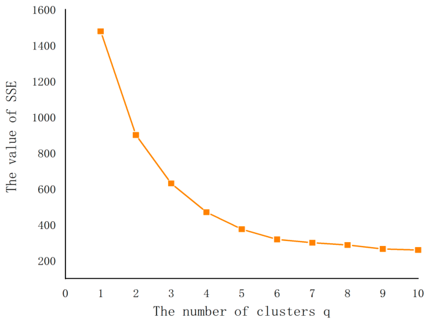
In the formula, c i is the i-th cluster center, and p i represents the aggregation of data points in the i-th cluster. As the number of clusters q increases, the samples are classified more accurately, and the SSE decreases. Theoretically, the smaller the SSE, the better the clustering effect. As the value of q increases to a certain level, the rate of the decline in SSE slows down. As shown in Figure 8, when q = 5 , it is the inflection point of the curve. The most suitable cluster number is 5.
In this paper, two clustering validity indicators are used to assess the quality of clustering: the Calinski–Harabasz indicator (CHI) and the Davies–Bouldi indicator (DBI). The CHI is obtained by the ratio of the compactness to the separation [38]. Thus, the larger the index is, the more compact the result is. The DBI metric estimates intraclass closeness by the distance from the sample point within a class to the center of the class to which it belongs, and the distance between class centers indicates the interclass dispersion [39]. Thus, the smaller the index is, the better the effect. Equations (37) to (38) describe these metrics:
C H I = T r ( B k ) T r ( W k ) × n k k 1
D B I = 1 k i = 1 k max j = 1 k , i j s i + s j c i c j 2 2

3.3. The Proposed CNN-IVIA-BLSTM Forecasting Model

Using the CNN-IVIA-BLSTM model to forecast the power load data:
Step 1. Feature fusion extraction. CNN is used to extract the data feature.
Step 2. Forecasting. IVIA optimizes the parameters related to the BLSTM network, then uses the optimized BLSTM to predict.
Step 3. Power load forecast evaluation. The load data forecasting effect analyzed using RMSE, MAE, and MAPE.

3.3.1. CNN: Convolutional Neural Network

A CNN can automatically extract potential features between massive loads of continuous and discontinuous data to build a compressed complete feature vector for the top fully connected layer [40]. It is a hierarchical neural feedforward network and consists of a series of network layers with different functions. It mainly comprises the input layer, implied layer, and output layer. Among these, the implied layer takes the convolutional layer as the core, and the main function of the convolution layer is to extract the feature fusion of the input data as an arithmetic of the convolution layer. In addition, the CNN includes pooling layers (to reduce the number of parameters of the neural network) and the Dropout layer (to prevent data overfitting). The 1D convolutional kernel is two-dimensional and has a length and width; however, there is a sliding window in the width or height direction, and multiplication is transformed into addition. In this paper, a 1D CNN is used, with a convolutional kernel size of 3 × 3 , a sliding window of 10, and a step size of 1. The overall structure of the convolutional network is shown in Figure 9. A convolutional block is a combination of M convolutional layers and b convergence layers. It can be stacked with N consecutive convolutional blocks followed by K fully connected layers.

3.3.2. BLSTM Bidirectional Long Short-Term Memory Network

BLSTM can remember a sequence well, can solve the dependency problem of longer time spans, and has a strong advantage in improving time series correlation. Based on the LSTM (long short-term memory) network, the forward and reverse network structures form a closed loop of information, which can better verify and correct the process error information while maintaining the bidirectional data information, which has stronger robustness [41]. The LSTM network structure is shown in Figure 10, and the relevant calculation equations are shown in (39)–(44).
I n p u t   g a t e :       i t = σ W i x t + U i h t 1 + b i
F o r g e t   g a t e :       f t = σ W f x t + U f h t 1 + b f
O u t p u t   g a t e :       o t = σ W 0 x t + U o h t 1 + b o
N e w   m e m o r y   u n i t :   c t = tanh W c x t + U c h t 1 + b c
F i n a l   m e m o r y   u n i t :   c t = f t c t 1 + i t c t
O u t p u t :         h t = o t tanh c t
where W i , W f , and W o represent input weight vectors; U i , U f , and U o represent upper output weight vectors; and b i , b f , b o , and b c are bias vectors. Sigmoid is generally selected as the excitation function for σ , which mainly plays a role of gating. It has an output between 0 and 1, which matches the physical definition of gating and is very close to 1 or 0 when the input is large or small, thus ensuring that the gate is open or closed. The tanh is an option to generate the new memory unit ct due to a faster convergence rate with an output between −1 and 1, which coincides with the center of the feature distribution being 0 in most scenarios. The related formulas are given in Equations (45) and (46):
s i g m o i d x = 1 1 + e x
tanh x = e x e x e x + e x
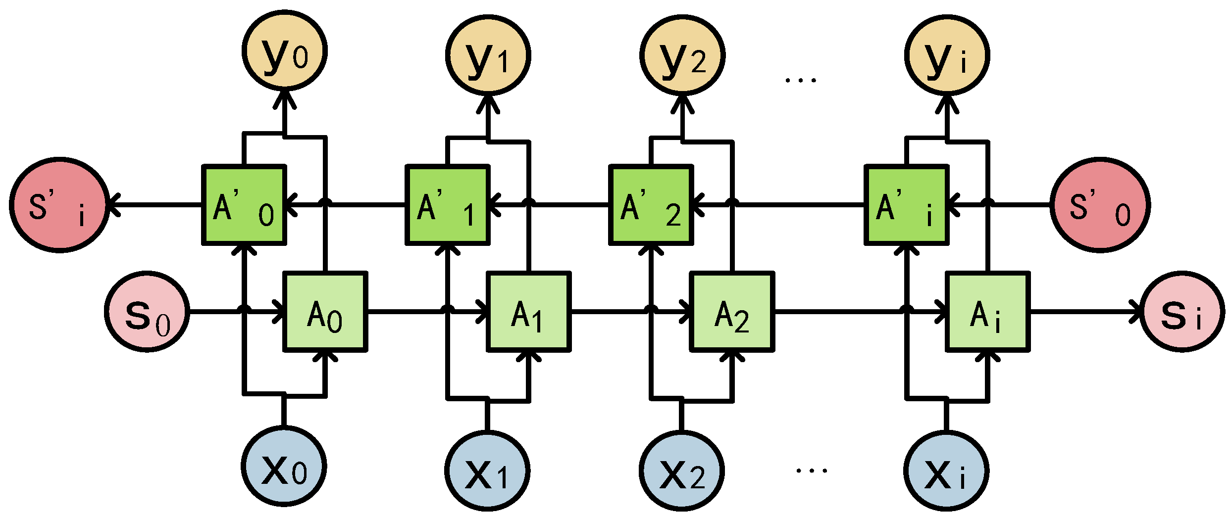
LSTM can only be passed in one direction, and the unit computation of the bidirectional neural network is connected with the unidirectional one. BLSTM consists of an input layer, forward LSTM layer, reverse LSTM layer, and output layer. However, the hidden layer of the bidirectional neural network must save two values, i.e., A , which is involved in the forward calculation, and A , which is involved in the reverse calculation. The final output value depends on the sum. The BLSTM network structure is shown in Figure 11.
However, a common problem is that BLSTM networks have many parameters, and without proper optimization, the model may be overfitted or slow to train, resulting in inefficiency. Too few nodes in the hidden layer will cause the model to not have the necessary learning ability and information processing capability, and too many nodes will increase the complexity of the network structure and make the learning process easily fall into local minima, which makes the network slow. When the learning rate is too high, the cost function is not easy to reduce to the lowest point, it is not easy to converge at the lowest point, and the convergence effect is poor. When too much training is performed, the gradient descent process may cross the nadir, which causes the training rate to be too low. In the case of reasonable tuning parameters, the more layers and neurons there are, the higher the accuracy rate; however, this can also lead to the overfitting phenomenon, and a regularization process can be used to solve the overfitting problem. In this paper, the number of implicit layer neurons, training times, learning rates, and regularization coefficients in BLSTM are optimized using the IVIA to improve the performance of the sequence modelling task.

3.3.3. Hybrid Forecasting Model

The CNN-IVIA-BLSTM model is a combined prediction model consisting of a CNN and BLSTM. BLSTM is a commonly used model architecture of deep learning models for sequence modelling tasks, and it has achieved good performance in many tasks. The CNN is first used to extract the feature vectors consisting of load influencing factors, which can be considered a “feature extractor”, then the extracted feature vectors are used for load prediction with the BLSTM model optimized by the IVIA. The hybrid prediction model structure is shown in Figure 12, which takes full advantage of both the CNN and BLSTM network to ensure the accuracy of the power load.
The forecasting steps are as follows:
  • Selected information as model input.
  • LVMD decomposes and denoises the original sequence, and DBFCM performs clustering.
  • The IVIA population size N, the maximum number of iterations M, and the initial search range of the parameters (the number of neurons in the hidden layer H, training number E, learning rate η , and regularization factor L 2 ) are set. The root mean square error ( y R M S E ) is used as the objective function in the optimization algorithm, and finally, the model of the influenza virus immunization algorithm coupled with the bidirectional long and short-term memory network is developed.
  • The 1D CNN reads the load sequence with a sliding time window of 10 and a step size of 1 for feature extraction.
  • m prediction models are obtained by inputting the CNN-IVIA-BLSTM prediction models for each component separately.
  • Finally, the predicted values of the m prediction models are combined to obtain the predicted values of the load.

3.3.4. Power Load Forecast Evaluation Indicator

Three evaluation indexes are set as y M A P E (mean absolute percentage error, MAPE), y R M S E (root mean square error, RMSE), and y M A E (mean absolute error, MAE). The equations are shown in (47) to (49):
y M A P E = 1 n i = 1 n | X a c t ( i ) X p r e d ( i ) X a c t ( i ) |
y R M S E = i = 1 n ( X a c t ( i ) X p r e d ( i ) ) 2 n
y M A E = 1 n i = 1 n | X a c t ( i ) X p r e d ( i ) |
In the above equation, n is the total number of predictions, X a c t ( i ) is the real value of the load at moment i, and X p r e d ( i ) is the predicted value of the load at moment i.

4. Case Analysis

In this paper, historical power load data from 2016 to 2018 in H city were used for prediction with a sampling interval of 15 min. LSTM, BLSTM, CNN-BLSTM, LVMD-DBFCM-CNN-BLSTM, and the proposed model in this paper are selected to compare the prediction results.

4.1. Analysis of Data Processing Results

4.1.1. Data Denoising and Decomposition

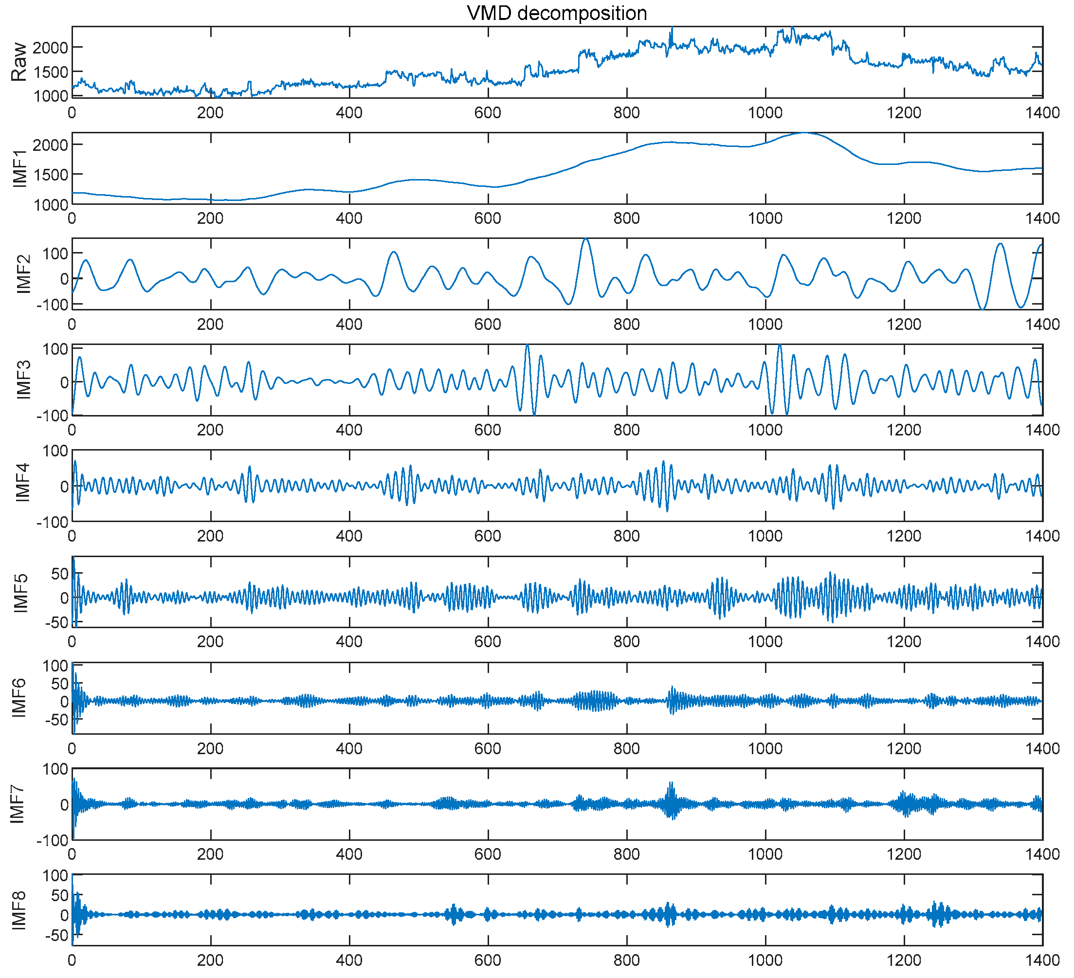
The original load data are decomposed and denoised using VMD, as shown in Figure 13, and the original load data sequence is decomposed into 8 IMF components. From the figure, we can see that the IMF7–IMF8 values are small and contain more noisy data, which are removed from the original data, then the first six IMF components are used to reconstruct the data to achieve data denoising.
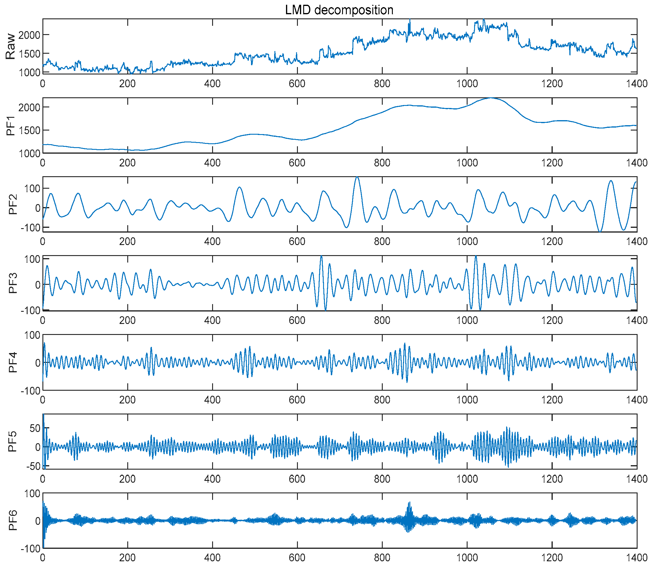
The second step of LVMD is to redecompose the denoised data with LMD. The denoised data are decomposed into a total of six PF components, and the decomposition results are shown in Figure 14. The values of PF1 are larger and maintain the same trend as the original data, containing the main valid information of the data. The values of PF2–PF6 are smaller, among which the periodic changes of PF2–PF4 are more obvious and PF6 is monotonically increasing, which is convenient for the prediction of each component. The randomness of the F5 sequence volatility is strong and the prediction accuracy of the F5 component is not high when making predictions.

4.1.2. Analysis of the Clustering Results

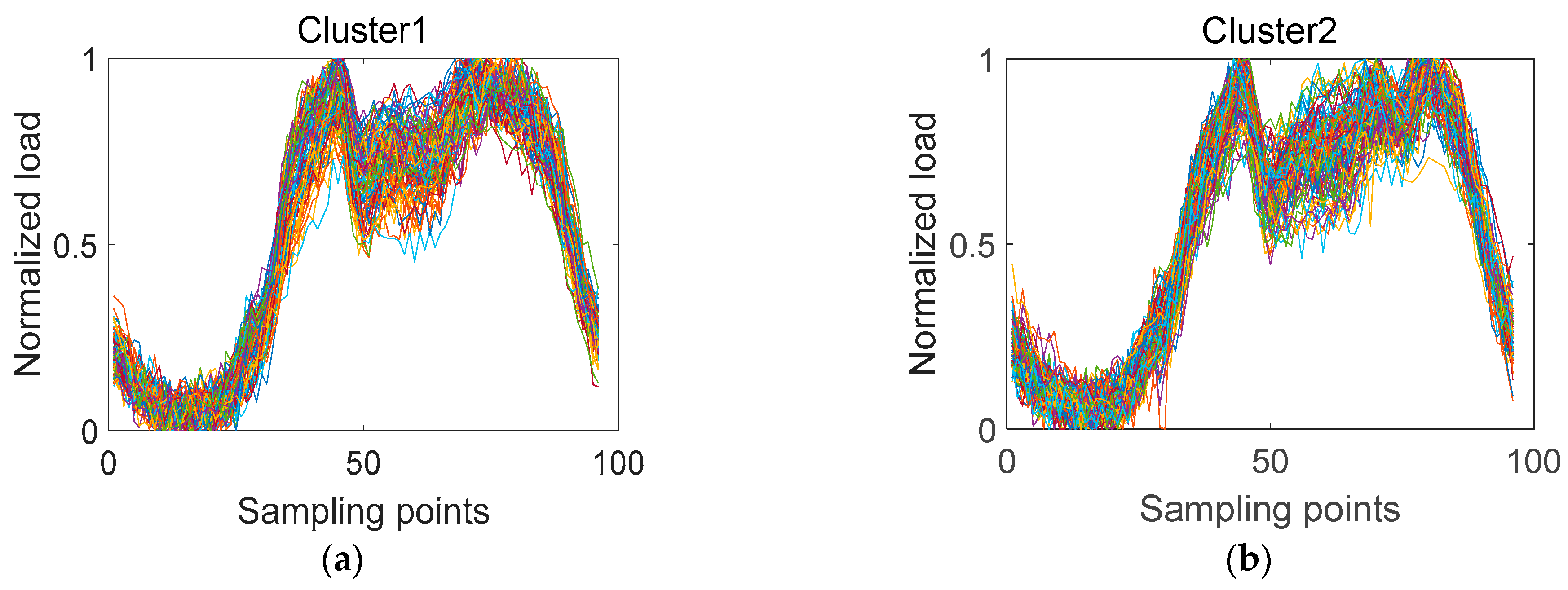
The daily load curve after LVMD-DBFCM clustering is shown in Figure 15.
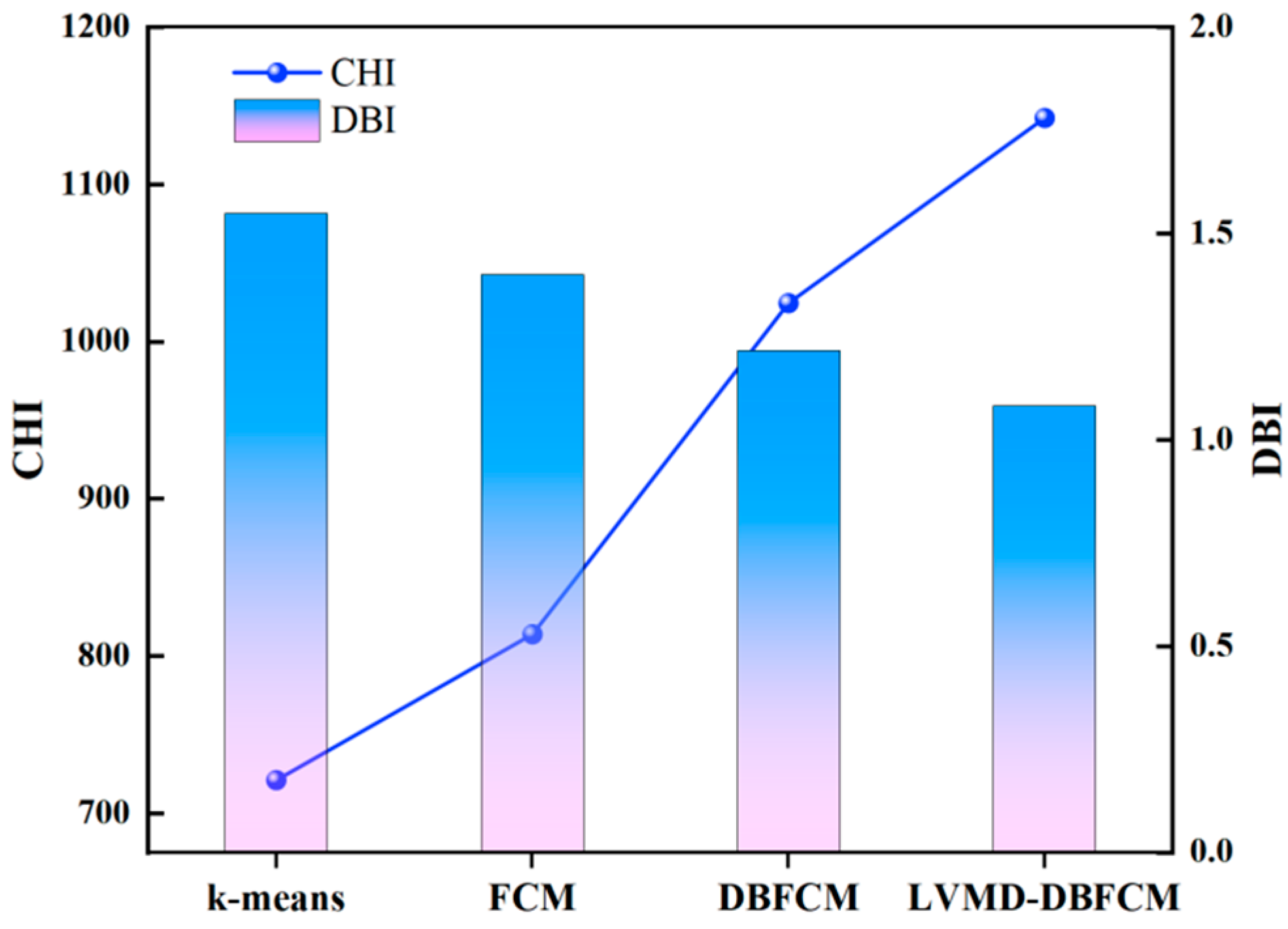
The clustering algorithm proposed in this paper is compared with k-means [42], FCM [43], and DBFCM. Their comparison is displayed in Table 3 and Figure 16. From the results, it can be seen that the maximum value of the CHI metric is 1142.509 and the minimum value of the DBI metric is 1.083. The clustering validity of the method proposed in this paper is better than that of the other three methods.

4.2. Analysis of the Prediction Results

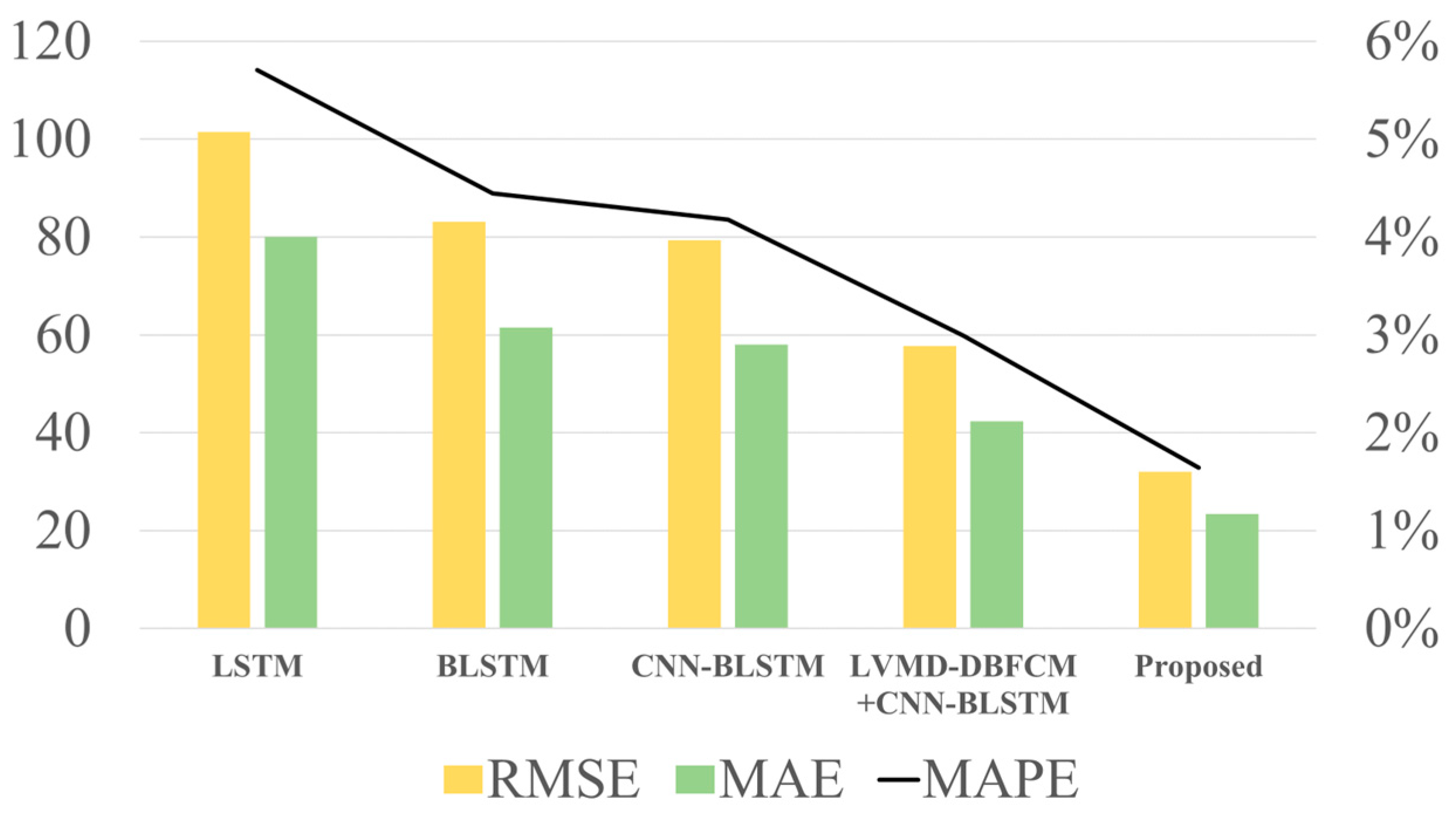
The comparison between the prediction model proposed in this paper and the four models LSTM, BLSTM, CNN-BLSTM, and LVMD-DBFCM+CNN-BLSTM using three load evaluation indices, RMSE, MAE, and MAPE, is shown in Table 4 and Figure 17. From the results, we can see that the prediction models proposed in this paper have better prediction results than the other four models in all evaluation indices.
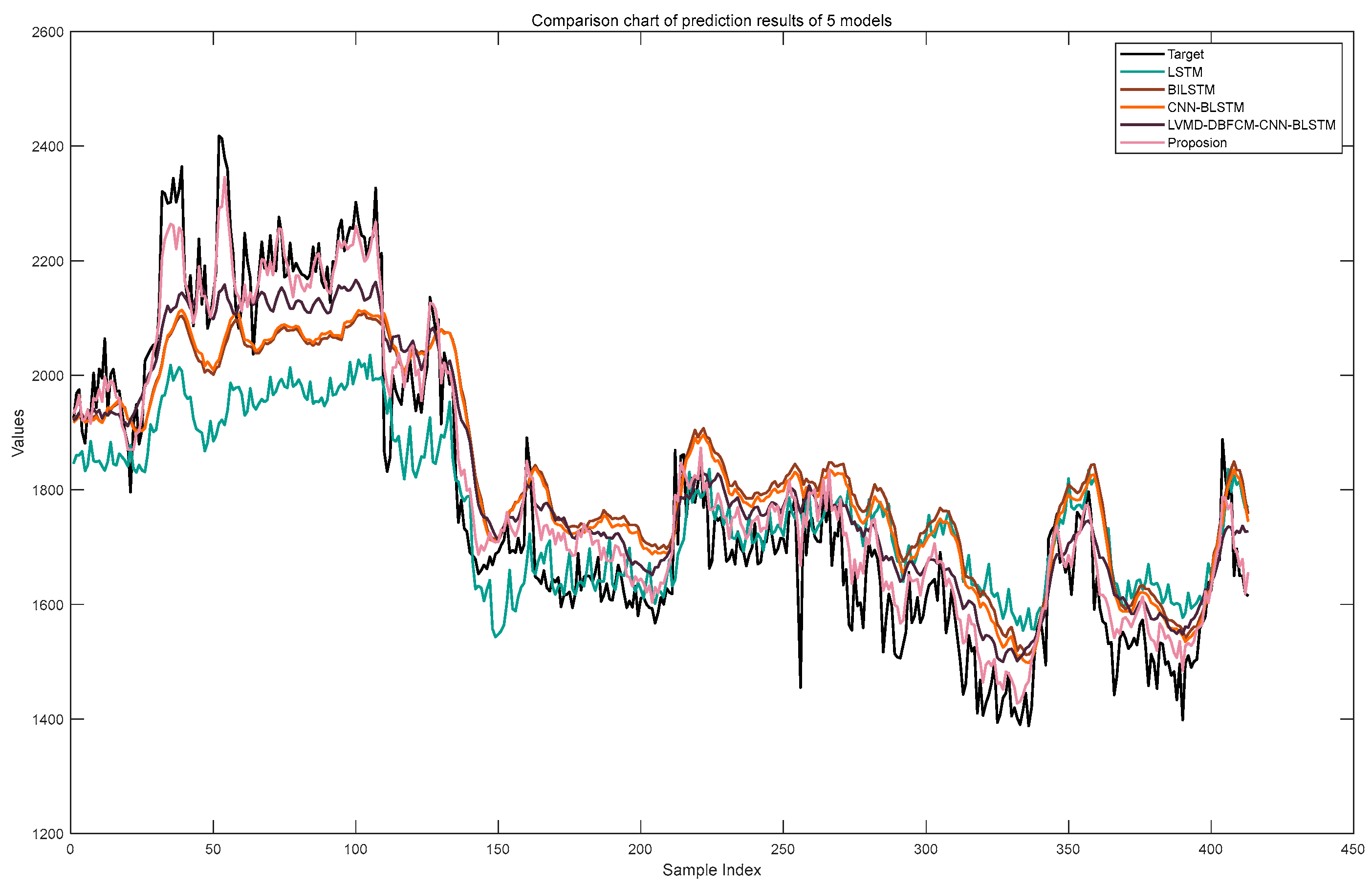
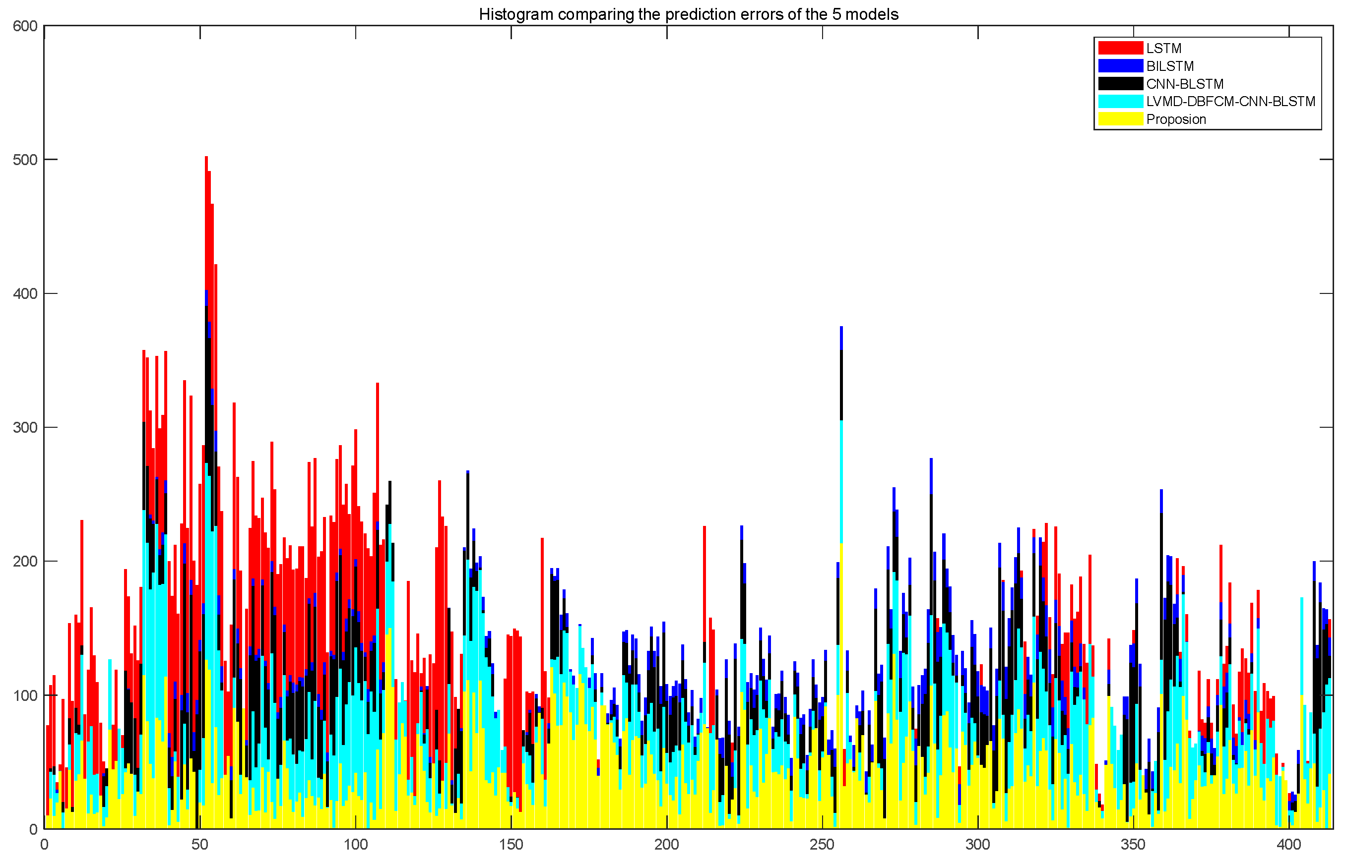
Figure 18 shows the prediction graphs of the five prediction models. From the figure, it can be clearly seen that the pink line, representing the model proposed in this paper, fits so closely to the target curve represented by the black line, which can better reflect the trend of the target, indicating that the model proposed in this paper has the better prediction effect than addressed models. Figure 19 shows the prediction error comparison of the 5 models, from which it can be clearly seen that the model proposed in this paper, represented by yellow, has the lowest error.

5. Conclusions

In this paper, a new model based on LVMD-DBFCM load curve clustering and a CNN-IVIA-BLSTM hybrid model for power load forecasting is proposed. This comprehensive technique takes historical load data and influencing factors (meteorology, economy, and data type) into account, where historical load data, meteorological factors, and economic factors are normalized, and the data types are uniquely heat coded.
The novel LVMD-DBFCM algorithm improves the continuity and stability of the data, and the values of the CHI and DBI quality assessment indicators are 1142.509 and 1.083, respectively, both of which reflect the good validity of the clustering method used in this paper. In the new CNN-IVIA-BLSTM model, a CNN is used for feature extraction, BLSTM is used for load forecasting, and the IVIA is used to optimize the relevant parameters in the BLSTM network. The results of the three electric load forecasting evaluation metrics of the hybrid forecasting model show that the RMSE is 31.9942, the MAE is 23.3691, and the MAPE is 1.6421%. The prediction effect of the electric load fits well with the target, and the prediction error is minimized.

Author Contributions

Conceptualization, L.H., J.W., Z.G. and T.Z.; Data curation, L.H., J.W., Z.G. and T.Z.; Formal analysis, L.H., J.W. and T.Z.; Investigation, L.H; Methodology, L.H. and J.W; Software, J.W. and Z.G.; Project administration, L.H.; Resources, L.H.; Supervision, L.H.; Validation, L.H.; Visualization, L.H.; Writing—original draft, L.H., J.W., Z.G. and T.Z.; Writing—review & editing, J.W. and Z.G. All authors have read and agreed to the published version of the manuscript.

Funding

This research received no external funding.

Institutional Review Board Statement

Not applicable.

Informed Consent Statement

Not applicable.

Data Availability Statement

Not applicable.

Conflicts of Interest

The authors declare no conflict of interest.

References

  1. Huang, Y. Medium-Long Term Power Load Forecasting of a Region. Master’s Thesis, Xihua University, Chengdu, China, 2015. [Google Scholar]
  2. Han, F.J.; Wang, X.H.; Qiao, J. Review on Artificial Intelligence based Load Forecasting Research for the New-type Power System. Proc. CSEE 2023, 1–24. [Google Scholar]
  3. Zhang, Y.; Wang, A.H.; Zhang, H. Overview of smart grid development in China. Power Syst. Prot. Control 2021, 49, 180–187. [Google Scholar]
  4. Gao, D.D.; Gao, S.T. Review on medium-long term power load forecasting study. Sci. Technol. Innov. Her. 2014, 11, 25. [Google Scholar]
  5. Shang, C.; Gao, J.; Liu, H.; Liu, F. Short-term load forecasting based on PSO-KFCM daily load curve clustering and CNN-LSTM model. IEEE Access 2021, 9, 50344–50357. [Google Scholar] [CrossRef]
  6. Huang, J.B. Based on trend extrapolation method analysis of city complexes load development characteristicsitle of the chapter. Rural Electrif. 2019, 7, 39–42. [Google Scholar]
  7. Song, F.; Liu, J.; Zhang, T. The Grey Forecasting Model for the Medium-and Long-Term Load Forecasting. J. Phys. Conf. Ser. 2020, 1654, 012104. [Google Scholar] [CrossRef]
  8. Fan, G.F.; Qing, S.; Wang, H. TSupport Vector Regression Model Based on Empirical Mode Decomposition and Auto Regression for Electric Load Forecasting. Energies 2013, 6, 1887–1901. [Google Scholar] [CrossRef]
  9. Qiu, X.P. Neural Network and Deep Learning. J. Chin. Inf. Process. 2020, 34, 4. [Google Scholar]
  10. Jarquin, C.S.S.; Gandelli, A.; Grimaccia, F.; Mussetta, M. Short-Term Probabilistic Load Forecasting in University Buildings by Means of Artificial Neural Networks. Forecasting 2023, 5, 390–404. [Google Scholar] [CrossRef]
  11. Liu, J.H. Power load forecasting in Shanghai based on CNN-LSTM combined model. Proc. SPIE 2022, 12254, 125–132. [Google Scholar]
  12. Li, J.W.; Luong, T.; Dan, J. When are tree structures necessary for deep learning of representations. In Proceedings of the 2015 Conference on Empirical Methods in Natural Language Processing, Lisbon, Portugal, 17–21 September 2015; Association for Computational Linguistics: Stroudsburg, PA, USA, 2015. [Google Scholar]
  13. Gu, H.C.; Mou, P.; Li, J.W. Modeling and application of ethylene cracking furnace based on cross-iterative BLSTM network. CIESC J. 2019, 70, 548–555. [Google Scholar]
  14. Xu, Y.; Xiang, Y.F.; Ma, T.X. Short-term Power Load Forecasting Method Based on EMD-CNN-LSTM Hybrid Model. J. North China Electr. Power Univ. 2022, 49, 81–89. [Google Scholar]
  15. Gao, W.C. Urban Gas Load Forecasting Based on EWT-CNN-LSTM Model. Master’s Thesis, Shanghai Normal University, Shanghai, China, 2021. [Google Scholar]
  16. Sun, G.L.; Li, B.J.; Xu, D.M.; Li, Y.P. Monthly Runoff Prediction Model Based on VMD-SSA-LSTM. Water Resour. Power 2022, 40, 18–21. [Google Scholar]
  17. Yang, Y. Research and Application of Medium and Long Term Load Forecasting Technology. Master’s Thesis, Shenyang Institute of Computing Technology, Chinese Academy of Science, Shenyang, China, 2021. [Google Scholar]
  18. Mojtaba, G.; Faraji, D.I.; Ebrahim, A.; Abolfazl, R. A novel and effective optimization algorithm for global optimization and its engineering applications: Turbulent Flow of Water-based Optimization (TFWO). Eng. Appl. Artif. Intell. 2020, 92. [Google Scholar] [CrossRef]
  19. Abdolkarim, M.B.; Mahmoud, D.N.; Adel, A. Golden eagle optimizer: A nature-inspired metaheuristic algorithm. Comput. Ind. Eng. 2021, 152, 107050. [Google Scholar]
  20. Mohamed, A.A.; Hassan, S.A.; Hemeida, A.M.; Alkhalaf, S. Parasitism-Predation algorithm (PPA): A novel approach for feature selection. Ain Shams Eng. J. 2019, 11, 293–308. [Google Scholar] [CrossRef]
  21. Dhiman, G.; Garg, M.; Nagar, A.; Kumar, V. A novel algorithm for global optimization: Rat Swarm Optimizer. J. Ambient Intell. Humaniz. Comput. 2020, 12, 8457–8482. [Google Scholar] [CrossRef]
  22. Mirjalili, S.; Mirjalili, S.M.; Lewis, A. Grey Wolf Optimizer. Adv. Eng. Softw. 2014, 69, 46–61. [Google Scholar] [CrossRef] [Green Version]
  23. Ramya, S.; Rajesh, N.B.; Viswanathan, B. Particle Swarm Optimization (PSO) based optimum Distributed Generation (DG) location and sizing for Voltage Stability and Loadability Enhancement in Radial Distribution System. Int. Rev. Autom. Control IREACO 2014, 7, 288–293. [Google Scholar]
  24. Jhila, N.; Modarres, K.F.; Akiko, Y. A whale optimization algorithm (WOA) approach for clustering. Cogent Math. Stat. 2018, 5, 1483565. [Google Scholar]
  25. Karol, S.; Ewelina, H.; Katarzyna, L.; Katarzyna, K. Spread of Influenza Viruses in Poland and Neighboring Countries in Seasonal Terms. Pathogens 2021, 10, 316. [Google Scholar]
  26. Oxford, J.S. Special Article: What Is the True Nature of Epidemic Influenza Virus and How Do New Epidemic Viruses Spread. Epidemiol. Infect. 1987, 99, 1–3. [Google Scholar] [CrossRef] [PubMed] [Green Version]
  27. Zhu, Z.W. Study on the Impact of Weather Factors on Characteristics of Electric Load. Ph.D. Thesis, Zhejiang University, Hangzhou, China, 2008. [Google Scholar]
  28. Xu, F.; Weng, G.Q. Research on Load Forecasting Based on CNN-LSTM Hybrid Deep Learning Model. In Proceedings of the 2022 IEEE 5th International Conference on Electronics Technology (ICET), Chengdu, China, 13–16 May 2022; pp. 1332–1336. [Google Scholar]
  29. Hu, Y.C. Research on Power Load Pattern Recognition Method Based on Improved k-means Clustering Algorithm. Master’s Thesis, University of Electronic Science and Technology of China, Chengdu, China, 2018. [Google Scholar]
  30. Zhang, H.; Zhang, Y.; Xu, Z. Thermal Load Forecasting of an Ultra-short-term Integrated Energy System Based on VMD-CNN-LSTM. In Proceedings of the 2022 International Conference on Big Data, Information and Computer Network (BDICN), Sanya, China, 20–22 January 2022; pp. 264–269. [Google Scholar]
  31. Dragomiretskiy, K.; Zosso, D. Variational mode decomposition. IEEE Trans. Signal Process. 2014, 62, 531–544. [Google Scholar] [CrossRef]
  32. Yang, S.S.; Zhou, H.; Zhao, H.Y. Fault diagnosis method for the bearing of reciprocating compressor based on LMD multiscale entropy and SVM. J. Mech. Transm. 2015, 39, 119–123. [Google Scholar]
  33. Wu, D.S.; Yang, Q.; Zhang, J.Y. Ensemble fault diagnosis method based on VMD-LMD-CNN. Bearing 2020, 10, 57–63. [Google Scholar]
  34. Li, P.S.; Li, X.R.; Chen, H.H. The characteristics classification and synthesis of power load based on fuzzy clustering. Proc. CSEE 2005, 25, 73–78. [Google Scholar]
  35. Zhou, K.L. Theoretical and Applied Research on Fuzzy C-means Clustering and Its Cluster Validation. Ph.D. Thesis, Hefei University of Technology, Hefei, China, 2014. [Google Scholar]
  36. Dong, T. Research on Electrical Load Pattern Recognition and Load Forecasting Based on Deep Learning. Master’s Thesis, Jilin University, Changchun, China, 2022. [Google Scholar]
  37. Ma, Z.B.; Xu, S.A.; Zhu, S.B. Power Load Classification Based on Feature Weighted Fuzzy Clustering. ELECTRIC POWER 2022, 55, 25–32. [Google Scholar]
  38. Tomasini, C.; Emmendorfer, L.; Borges, E.N. A methodology for selecting the most suitable cluster validation internal indices. In Proceedings of the 31st Annual ACM Symposium on Applied Computing (SAC ′16), Pisa, Italy, 4–8 April 2016; pp. 901–903. [Google Scholar]
  39. Hao, X.H.; Li, Y.L.; Gu, Q. Power load data clustering algorithm based on DTW histogram. Transducer Microsyst. Technol. 2020, 39, 140–142. [Google Scholar]
  40. Liu, Y.H.; Zhao, Q. Ultra-short-term power load forecasting based on cluster empirical mode decomposition of CNN-LSTM. Power Syst. Technol. 2021, 45, 4444–4451. [Google Scholar]
  41. Zhu, H.S. Design and Implementation of CNN-BLSTM Speech Separation Algorithm Fused With Self-attention Mechanism. Master’s Thesis, Hebei University of Science and Technology, Shijiazhuang, China, 2021. [Google Scholar]
  42. Wang, J.D.; Gu, Z.C.; Ge, L.J. Load Clustering Characteristic Analysis of the Distribution Network Based on the Combined Improved Firefly Algorithm and K-means Algorithm. J. Tianjin Univ. Sci. Technol. 2023, 56, 137–147. [Google Scholar]
  43. Pan, X.G. Research of Fuzzy Clustering Algorithm on Complicated Data and Feature Weight Learning Techniques. Ph.D. Thesis, Jiangnan University, Wuxi, China, 2022. [Google Scholar]
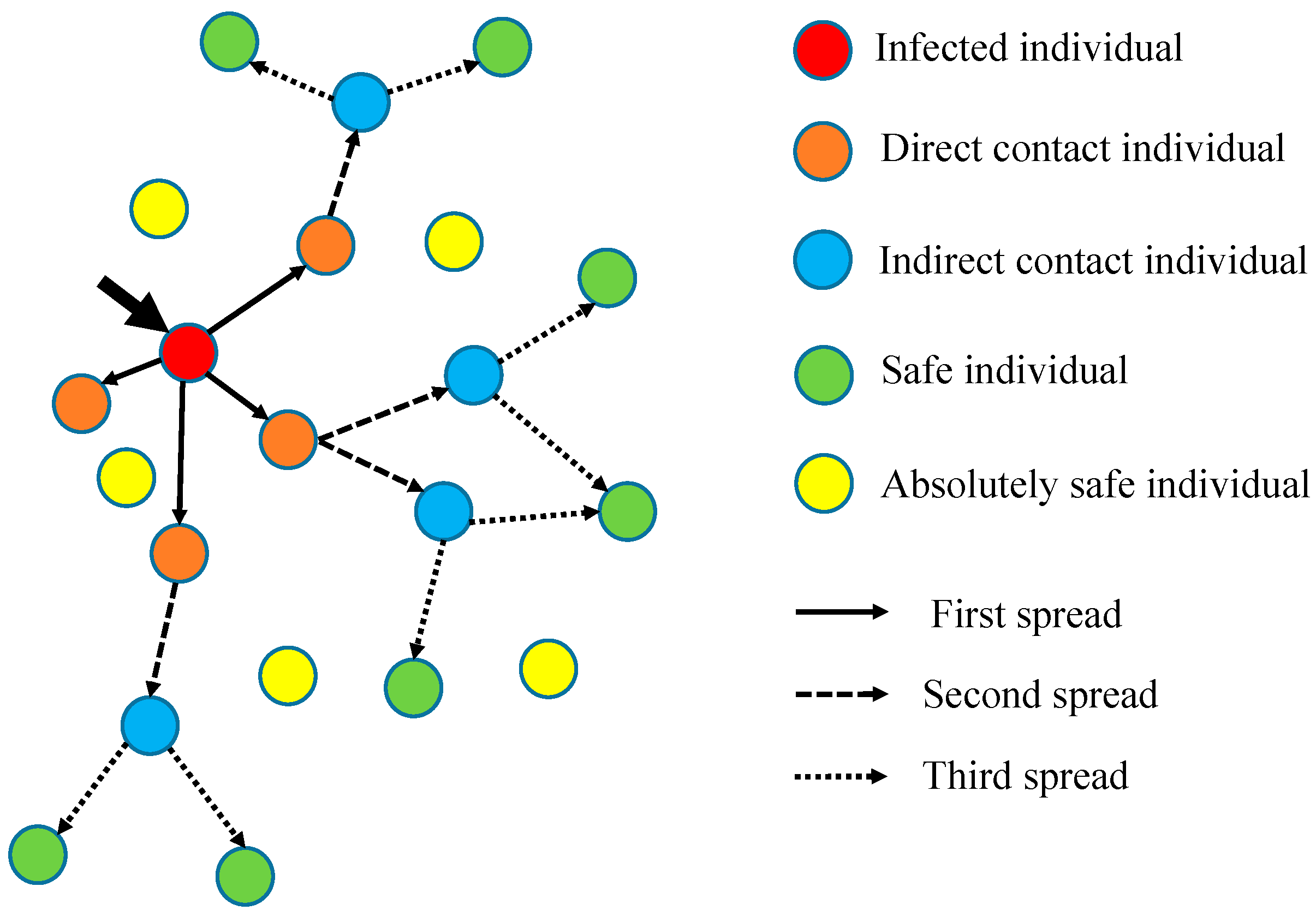
Figure 1. Diagram of the process of influenza virus population transmission.
Applsci 13 07332 g001
Figure 2. Diagram of the virus cell exchange process.
Applsci 13 07332 g002
Figure 3. The proportion of immune individuals in the whole population.
Applsci 13 07332 g003aApplsci 13 07332 g003b
Figure 4. Growth curve of the number of infected people.
Applsci 13 07332 g004
Figure 5. Standard test function optimization result.
Applsci 13 07332 g005aApplsci 13 07332 g005b
Figure 6. The overall structure design of this paper.
Applsci 13 07332 g006
Figure 7. Distribution of whole load data in the dataset for 15 min. (a) Data from 00:00 to 12:00; (b) Data from 12:00 to 23:45. Box-whisker plot, the dots replace the abnormal value, the middle line of the box is he median of the data, which represents the average level of the sample data.
Applsci 13 07332 g007
Figure 8. The gradient graph of SSE with increasing cluster number q from 1 to 10.
Applsci 13 07332 g008
Figure 9. Overall structure of a CNN.
Applsci 13 07332 g009
Figure 10. LSTM network structure diagram.
Applsci 13 07332 g010
Figure 11. BLSTM network structure diagram.
Applsci 13 07332 g011
Figure 12. Hybrid forecasting model structure diagram.
Applsci 13 07332 g012
Figure 13. Result of VMD decomposition.
Applsci 13 07332 g013
Figure 14. Result of LMD decomposition.
Applsci 13 07332 g014
Figure 15. (ae) Daily load curve after LVMD-DBFCM clustering when the number of clusters is determined to be 5.
Applsci 13 07332 g015aApplsci 13 07332 g015b
Figure 16. Comparative graph displaying the clustering validity indicators, CHI and DBI, of the K-means, FCM, DBFCM, and LVMD-DBFCM methods.
Applsci 13 07332 g016
Figure 17. Comparison of the RMSE, MAE, and MAPE results for 5 models’ predictions.
Applsci 13 07332 g017
Figure 18. Comparison chart of the prediction results of 5 models.
Applsci 13 07332 g018
Figure 19. Comparison of prediction errors of the 5 models.
Applsci 13 07332 g019
Table 1. Standard test function.
StandardDimensionSearch SpaceMinimum
F 1 ( x ) = i = 1 n x i 2 30[−100, 100]0
F 2 ( x ) = i = 1 n x i + i = 1 n x i 30[−10, 10]0
F 3 ( x ) = i = 1 n j = 1 n x j 2 30[−100, 100]0
F 4 ( x ) = max i x i ,   1 i n 30[−100, 100]0
F 5 ( x ) = i = 1 n 1 100 ( x i + 1 x i 2 ) + ( x i 1 ) 2 30[−30, 30]0
F 6 ( x ) = i = 1 n x i + 0.5 2 30[−100, 100]0
F 7 ( x ) = i = 1 n i x i 4 + r a n d o m [ 0 , 1 ) 30[−128, 128]0
F 8 ( x ) = i = 1 n x i sin x i 30[−500, 500]−12,569.5
F 9 ( x ) = i = 1 n x i 2 10 cos ( 2 π x i ) + 10 30[−5.12, 5.12]0
F 10 ( x ) = 20 exp 0.2 1 n i = 1 n x i 2 exp 1 n i = 1 n cos 2 π x i + 20 + e 30[−32, 32]0
F 11 ( x ) = 1 4000 i = 1 n x i 2 i = 1 n cos x i i + 1 30[−600, 600]0
F 12 ( x ) = π n 10 sin ( π y 1 ) + i = 1 n 1 ( y i 1 ) 2 1 + 10 sin 2 ( π y i + 1 ) + y n 1 2 + i = 1 n u ( x i ,   10 ,   100 ,   4 ) y i = 1 + x i + 1 4 u ( x i ,   a ,   k ,   m ) = k ( x i a ) m x i > a 0 a < x i < a k ( x i a ) m x i < a 30[−50, 50]0
F 13 ( x ) = 0.1 sin 2 ( 3 π x i ) + i = 1 n ( x i 1 ) 2 1 + sin 2 ( 3 π x i + 1 ) + ( x n 1 ) 2 1 + sin 2 ( 2 π x n ) + i = 1 n u ( x i ,   5 ,   100 ,   4 ) 30[−50, 50]0
F 14 ( x ) = 1 500 + j = 1 25 1 j + i = 1 2 ( x i a i j ) 6 1 2[−65.56, 65.56]1
F 15 ( x ) = i = 1 11 a i x 1 ( b i 2 + b i x 2 ) b i 2 + b i x 3 + x 4 2 4[−5, 5]0.0003075
F 16 ( x ) = 4 x 1 2 2.1 x 1 4 + 1 3 x 1 6 + x 1 x 2 4 x 2 2 + 4 x 2 4 2[−5, 5]−1.0316
F 17 ( x ) = x 2 5.1 4 π 2 x 1 2 + 5 π x 1 6 2 + 10 1 1 8 π cos x 1 + 10 2[−5, 5]0.398
F 18 ( x ) = 1 + ( x 1 + x 2 + 1 ) 2 ( 19 14 x 1 + 3 x 1 2 14 x 2 + 6 x 1 x 2 + 3 x 2 2 ) × 30 + ( 2 x 1 3 x 2 ) 2 ( 18 32 x 1 + 12 x 1 2 + 48 x 2 36 x 1 x 2 + 27 x 2 2 ) 2[−2, 2]3
F 19 ( x ) = i = 1 4 c i   exp j = 1 3 a i j ( x j p i j ) 2 3[1, 3]−3.86
F 20 ( x ) = i = 1 4 c i   exp j = 1 6 a i j ( x j p i j ) 2 6[0, 1]−3.32
F 21 ( x ) = i = 1 10 j = 1 5 x j C j i 2 + β i 1 β = 1 10 ( 1 ,   2 ,   2 ,   4 ,   4 ,   6 ,   3 ,   7 ,   5 ,   5 ) C = 4.0 1.0 8.0 6.0 3.0 2.0 5.0 8.0 6.0 7.0 4.0 1.0 8.0 6.0 7.0 9.0 3.0 1.0 2.0 3.6 4.0 1.0 8.0 6.0 3.0 2.0 5.0 8.0 6.0 7.0 4.0 1.0 8.0 6.0 7.0 9.0 3.0 1.0 2.0 3.6 4[0, 10]−10.1532
F 22 ( x ) = i = 1 7 j = 1 5 x j C j i 2 + β i 1 4[0, 10]−10.4028
F 23 ( x ) = i = 1 10 j = 1 4 x j C j i 2 + β i 1 4[0, 10]−10.5364
Table 2. Results of the testing functions optimized by different algorithms.
F IVIATFWOGEOPPARSOGWOPSOWOA
optimal0.000 × 1000.000 × 1005.988 × 10−60.000 × 1000.000 × 1000.000 × 1008.428 × 10−50.000 × 100
F1average1.820 × 10−2484.900 × 10−12.136 × 10−11.598 × 10−69.458 × 10−1021.985 × 10−476.789 × 10−129.486 × 10−71
worst1.245 × 10−1623.500 × 10−115.121 × 10−12.185 × 10−11.169 × 10−138.942 × 10−108.628 × 10−186.839 × 10⁻²⁷
optimal0.000 × 1000.000 × 1000.000 × 1000.000 × 1000.000 × 1006.843 × 10−366.880 × 10−101.642 × 10−104
F2average9.840 × 10−531.249 × 10−84.878 × 10−69.785 × 10−71.854 × 10−366.842 × 10−136.874 × 10−74.859 × 10−47
worst2.350 × 10−301.895 × 10−61.236 × 10−48.545 × 10−51.561 × 10−186.842 × 10−66.420 × 10−46.465 × 10⁻²⁸
optimal0.000 × 1002.855 × 10−11.565 × 1011.585 × 10−71.265 × 10−66.872 × 10−34.265 × 10−21.063 × 103
F3average4.185 × 10−111.522 × 1005.016 × 1021.855 × 10−51.295 × 10−63.000 × 1012.326 × 1013.064 × 103
worst1.855 × 10−85.489 × 1001.000 × 1051.855 × 10−31.486 × 10−31.014 × 1026.019 × 1011.036 × 104
optimal9.459 × 10−771.125 × 1002.153 × 1002.126 × 1003.165 × 10−32.894 × 10−248.486 × 10−23.492 × 10−1
F4average5.895 × 10−342.459 × 1004.153 × 1003.124 × 1002.989 × 1001.987 × 10−141.425 × 1009.482 × 10−1
worst2.349 × 10−193.157 × 1008.166 × 1005.156 × 1006.362 × 1006.850 × 10−76.895 × 1003.843 × 100
optimal9.646 × 10−102.360 × 10−11.465 × 1011.946 × 1001.235 × 1002.169 × 1009.892 × 10−11.979 × 100
F5average5.419 × 10−86.523 × 1005.988 × 1021.249 × 1011.565 × 1011.249 × 1011.468 × 1019.162 × 100
worst1.242 × 10−22.104 × 1011.275 × 1041.991 × 1011.035 × 1025.616 × 1012.317 × 1013.216 × 101
optimal2.355 × 10−183.985 × 10−48.852 × 10−21.289 × 10−31.965 × 10−63.687 × 10−17.985 × 10−106.485 × 10⁻²
F6average9.475 × 10−109.125 × 10−18.049 × 10−21.597 × 10−11.547 × 10−19.006 × 10−17.864 × 10−79.717 × 10⁻¹
worst9.855 × 10−51.836 × 1003.598 × 1001.099 × 1006.218 × 10−12.663 × 1006.843 × 10−22.097 × 100
optimal1.968 × 10−70.000 × 1003.942 × 10−23.975 × 10−64.885 × 10−33.946 × 10−39.847 × 10−53.550 × 10⁻⁵
F7average2.495 × 10−31.698 × 10−13.965 × 10−13.735 × 10−11.125 × 10−28.972 × 10−18.885 × 10−14.165 × 10⁻¹
worst6.515 × 10−11.317 × 1001.569 × 1001.032 × 1003.339 × 10−11.398 × 1001.763 × 1001.223 × 100
optimal−1.256 × 10⁴−1.024 × 10⁴−5.663 × 10³−1.124 × 10⁴−1.035 × 10⁴−9.176 × 10³−1.034 × 10⁴−1.224 × 10⁴
F8average−1.156 × 10⁴−9.563 × 10³−4.983 × 10³−8.832 × 10³−8.865 × 10³−5.863 × 10³−6.856 × 10³−8.936 × 10³
worst−1.055 × 10⁴−7.934 × 10³−3.527 × 10³−7.295 × 10³−5.235 × 10³−4.330 × 10³−5.845 × 10³−7.532 × 10³
optimal0.000 × 1004.946 × 10−69.533 × 10−70.000 × 1001.968 × 10−226.427 × 10−36.848 × 10−87.842 × 10⁻²⁸
F9average5.649 × 10−51.568 × 10−33.798 × 10−31.765 × 10−31.765 × 10−63.499 × 10−53.492 × 10−49.787 × 10⁻⁹
worst3.476 × 10−21.065 × 1009.833 × 10−13.177 × 10−21.685 × 10−11.297 × 1001.379 × 10−13.790 × 10⁻³
optimal9.852 × 10−214.682 × 10−111.649 × 10−46.842 × 10−89.845 × 10−65.400 × 10−166.463 × 10−56.842 × 10−15
F10average1.855 × 10−84.190 × 10−31.515 × 10−16.850 × 10−39.815 × 10−28.943 × 10−33.163 × 10−38.463 × 10⁻⁸
worst1.642 × 10−51.684 × 10−11.331 × 1001.146 × 1003.855 × 10−16.315 × 10−19.198 × 10−16.318 × 10⁻³
optimal5.989 × 10 −99.847 × 10−55.646 × 10−31.685 × 10−79.946 × 10−53.489 × 10−23.965 × 10−43.787 × 10⁻⁹
F11average3.500 × 10−83.490 × 10−13.654 × 1014.846 × 10−41.654 × 10−33.326 × 10−11.038 × 1009.779 × 10−5
worst1.985 × 10−42.165 × 1001.068 × 1023.168 × 1005.486 × 10−11.235 × 1001.380 × 1003.480 × 10−3
optimal5.648 × 10−122.165 × 10−66.846 × 1016.546 × 10−76.468 × 10−74.893 × 10−84.896 × 10−131.687 × 10⁻³
F12average6.942 × 10−81.656 × 10−36.845 × 1028.646 × 10−56.579 × 10−47.893 × 1084.987 × 10−106.447 × 10⁻¹
worst1.685 × 10−49.924 × 10−21.007 × 1041.634 × 10−16.846 × 10−23.589 × 10−34.983 × 10−71.349 × 100
optimal6.115 × 10−84.216 × 10−52.647 × 1015.242 × 10−25.464 × 10−44.685 × 10−44.165 × 10−74.198 × 10−8
F13average4.359 × 10−206.410 × 10−31.464 × 1025.825 × 1001.351 × 10−23.199 × 10−34.147 × 10−44.168 × 10⁻⁶
worst4.642 × 10−81.416 × 1001.001 × 1042.353 × 1013.861 × 1002.056 × 1001.325 × 1009.650 × 10−3
optimal1.000 × 1001.000 × 1001.001 × 1001.024 × 1001.115 × 1001.259 × 1001.000 × 1001.000 × 100
F14average1.001 × 1001.674 × 1001.009 × 1002.196 × 1001.351 × 1001.950 × 1001.350 × 1001.268 × 100
worst1.007 × 1002.419 × 1002.486 × 1001.117 × 1012.652 × 1001.286 × 1012.149 × 1001.635× 108
optimal3.000 × 10−45.419 × 10−41.684 × 10−36.554 × 10−43.948 × 10−49.157 × 10−49.165 × 10−33.917 × 10⁻⁴
F15average3.425 × 10−48.646 × 10−31.682 × 10−36.834 × 10−36.422 × 10−22.925 × 10−36.117 × 10−39.164 × 10⁻³
worst6.453 × 10−36.550 × 10−11.954 × 10−19.846 × 10−29.648 × 10−11.896 × 10−11.430 × 10−29.168 × 10⁻²
optimal−1.032 × 100−9.186 × 10⁻¹−1.021 × 100−1.001 × 100−9.425 × 10⁻¹−9.168 × 10⁻¹−8.250 × 10⁻²−1.000 × 100
F16average−1.000 × 100−8.634 × 10⁻¹−9.648 × 10⁻¹−9.545 × 10⁻¹−8.217 × 10⁻¹−2.198 × 10⁻¹−1.625 × 10⁻⁸−5.491 × 10⁻¹
worst4.618 × 10−1−5.462 × 10⁻¹−6.139 × 10⁻¹−8.316 × 10⁻¹−7.717 × 10−11.198 × 10−11.032 × 100−1.493 × 10⁻¹
optimal3.981 × 10−34.856 × 10−24.404 × 10−14.040 × 10−13.990 × 10−24.299 × 10−14.399 × 10−13.992 × 10⁻¹
F17average4.040 × 10−24.000 × 10−26.004 × 10−16.040 × 10−18.036 × 10−16.498 × 10−19.413 × 10−11.065 × 100
worst5.033 × 10−19.911 × 10−11.032 × 1002.030 × 1001.603 × 1002.064 × 1002.319 × 1001.916 × 100
optimal3.000 × 1003.005 × 1003.016 × 1003.149 × 1003.001 × 1003.198 × 1003.616 × 1003.264 × 100
F18average3.015 × 1003.147 × 1003.656 × 1003.648 × 1003.004 × 1003.616 × 1004.086 × 1003.949 × 100
worst3.146 × 1003.142 × 1004.411 × 1004.245 × 1003.133 × 1004.691 × 1004.620 × 1005.017 × 100
optimal−3.860 × 100−3.861 × 100−3.195 × 100−3.619 × 100−3.812 × 100−3.852 × 100−3.801 × 100−3.859 × 100
F19average−3.677 × 100−3.852 × 100−2.870 × 100−3.595 × 100−3.816 × 100−3.742 × 100−3.550 × 100−3.726 × 100
worst−3.165 × 100−3.832 × 100−8.456 × 10⁻¹−3.455 × 100−3.795 × 100−3.516 × 100−2.949 × 100−3.030 × 100
optimal−3.320 × 100−3.146 × 100−3.307 × 100−3.032 × 100−2.919 × 100−1.982 × 100−2.098 × 100−3.156 × 100
F20average−2.996 × 100−2.920 × 100−3.019 × 100−2.533 × 100−1.398 × 100−1.089 × 100−9.497 × 10⁻¹−1.979 × 100
worst−2.649 × 100−2.520 × 100−2.120 × 1001.298 × 100−5.945 × 10−11.685 × 10−1−6.430 × 10⁻²−1.189 × 100
optimal−1.015 × 101−1.007 × 101−1.002 × 101−1.015 × 101−8.103 × 100−1.002 × 101−9.162 × 100−1.006 × 101
F21average−9.122 × 100−9.004 × 100−9.654 × 100−1.012 × 101−4.137 × 100−8.981 × 100−7.198 × 100−9.682 × 100
worst−7.596 × 100−5.642 × 100−8.514 × 100−9.632 × 100−6.517 × 10⁻¹−1.192 × 100−1.192 × 100−8.336 × 100
optimal−1.040 × 101−1.032 × 101−1.035 × 101−1.040 × 101−1.039 × 101−1.032 × 101−9.198 × 100−1.006 × 101
F22average−1.015 × 101−8.250 × 100−1.015 × 101−5.365 × 100−3.349 × 100−9.195 × 100−6.927 × 100−8.198 × 100
worst−1.002 × 101−4.820 × 100−9.671 × 100−2.389 × 10−18.924 × 10−2−4.928 × 100−1.162 × 100−1.265 × 10⁻¹
optimal−1.052 × 101−9.525 × 100−1.051 × 101−8.449 × 100−1.046 × 101−1.000 × 101−9.198 × 100−9.062 × 100
F23average−1.025 × 101−6.489 × 100−1.050 × 101−4.168 × 100−6.265 × 100−5.984 × 100−3.198 × 10⁻¹−6.894 × 100
worst−9.219 × 100−1.220 × 100−9.647 × 100−1.608 × 10⁻¹−2.487 × 10⁻¹−1.963 × 10−11.625 × 10−2−1.820 × 100
Table 3. The comparative table displaying the clustering validity indicators, CHI and DBI, of the K-means, FCM, DBFCM, and LVMD-DBFCM methods.
MethodsCHIDBI
K-means721.2011.549
FCM814.0141.401
DBFCM1024.7431.216
LVMD-DBFCM1142.5091.083
Table 4. The comparative table displaying the clustering validity indicators, CHI and DBI, of the K-means, FCM, DBFCM, and LVMD-DBFCM methods.
ModelsRMSEMAEMAPE
LSTM101.481780.09805.7087%
BLSTM83.149861.48264.4460%
CNN-BLSTM79.334058.02454.1782%
LVMD-DBFCM+CNN-BLSTM57.731642.36692.9946%
Proposed31.994223.36911.6421%
Disclaimer/Publisher’s Note: The statements, opinions and data contained in all publications are solely those of the individual author(s) and contributor(s) and not of MDPI and/or the editor(s). MDPI and/or the editor(s) disclaim responsibility for any injury to people or property resulting from any ideas, methods, instructions or products referred to in the content.