In Vivo Bone Progression in and around Lattice Implants Additively Manufactured with a New Titanium Alloy

Abstract

The osseointegration in/around additively manufactured (AM) lattice structures of a new titanium alloy, Ti–19Nb–14Zr, was evaluated. Different lattices with increasingly high sidewalls gradually closing them were manufactured and implanted in sheep. After removal, the bone–interface implant (BII) and bone–implant contact (BIC) were studied from 3D X-ray computed tomography images. Measured BII of less than 10 µm and BIC of 95% are evidence of excellent osseointegration. Since AM naturally leads to a high-roughness surface finish, the wettability of the implant is increased. The new alloy possesses an increased affinity to the bone. The lattice provides crevices in which the biological tissue can jump in and cling. The combination of these factors is pushing ossification beyond its natural limits. Therefore, the quality and speed of the ossification and osseointegration in/around these Ti–19Nb–14Zr laterally closed lattice implants open the possibility of bone spline key of prostheses. This enables the stabilization of the implant into the bone while keeping the possibility of punctual hooks allowing the implant to be removed more easily if required. Thus, this new titanium alloy and such laterally closed lattice structures are appropriate candidates to be implemented in a new generation of implants.

1. Introduction

Additive manufacturing (AM) enables the manufacture of very complex shapes and alloys [1,2]. More specifically, the laser-based powder bed fusion process [3,4,5], due to its implementation of small grain size powder (15–45 µm) allowing small and thin structures to be manufactured, enables the fabrication of lattice structures. Such structures are likely to promote bone growth in implantology. This bodes for the stability of the implant, which is a very interesting aspect for the medical sector. Indeed, better and faster osseointegration of the implant into the human body allows the patient to recover faster. In a previous article [6], we already demonstrated “in vivo” that the lattice promotes osseointegration by implementing the titanium alloy Ti6Al4V grade 23 containing aluminum (Al) and vanadium (V), already widely used for dental and hip implants. This study concerned mainly the conformity of the implants to their computer-aided design (CAD) and the powder particle adhesion to the lattices, and investigated the osseointegration as a function of the shape and size of the lattice cells. The bone formation was only qualitatively studied by visual observations on X-ray computed tomography (XCT) images of the implants placed in a sheep for eight weeks. A stop of the bone growth was observed at 3 mm from the border in the lattice of 1200 µm cell size after 8 weeks, in the Ti6Al4V alloy.

In the present work, specimens with the same geometrical configuration (same CAD, same shape and size of the lattice cells) as the previous work and a new-patented titanium alloy for implant Ti–19Nb–14Zr [7], called ZTM14N, containing niobium (Nb) and zirconium (Zr) instead of Al and V were investigated. This material, studied from a mechanical point of view by the French National Center for Scientific Research (CNRS) according to ASTM standards [8], reveals very interesting mechanical properties, as shown in Appendix A. For example, it has a lower elastic modulus (38 GPa) than other titanium alloys (100 to 130 GPa for Ti6Al4V [9]). In addition, it contains highly biocompatible materials [10] and is highly resistant to corrosion [11,12]. According to Kurtz et al. [11,12], ZTM14N is ten times more resistant to inflammation than Ti6Al4V. Such properties make the ZTM14N alloy the best alternative material for the medical market. Indeed, a significant stiffness mismatch between the human bone (25–30 GPa) and the implant material causes a stress effect that leads to bone resorption. Bone resorption can be detrimental when the degradation of existing bone predominates over bone formation. Furthermore, the release of both V and Al ions from Ti6Al4V in the human body might cause long-term health problems, such as peripheral neuropathy, osteomalacia, and Alzheimer’s disease [13,14].

In addition, the duration of the implantation concerned two sheep and lasted twelve weeks instead of eight weeks in the previous study. This longer residence time is the classical duration fracture consolidation.

Finally, the specimens are surrounded by increasingly high sidewalls gradually closing the lattice structures.

The purpose of this new study was twofold. First, the study of the contact between the bone and the implant from two points of view: (1) the bone–interface implant (BII), i.e., the interface thickness between bone and implant surfaces, and (2) determined from BII, the bone–implant contact (BIC), i.e., the proportion of the implant surface in contact with bone. Second, the study of the bone progression in depth as a function of the lattice access, as well as a function of bone location in the body (tibia or metatarsal bone).

The histomorphometry of the BIC, i.e., the ratio of bone over metal, is traditionally performed by microscopy on prepared glass slides, and it is by nature two-dimensional (2D). In this work, the study is performed on XCT images segmented implementing machine learning (ML) algorithms. Thus, the study is performed from three-dimensional (3D) and statistically sounder (large volumes). However, the BII study is performed meticulously on 2D slices that can be extracted in any direction from these 3D images.

To summarize, in order to study the benefit of new titanium alloy lattice structures, gradually laterally closed, on osseointegration, the methodology implemented was to implant ZTM14N lattice specimens, more or less laterally closed, in the tibia and metatarsal bone of two sheep for twelve weeks. Then, after the removal of the specimens, the contact between the bone and the implant and the bone progression in depth from XCT images segmented with ML were studied.

This article will address the materials and methods, including the implants with a lattice structure design and fabrication in the new titanium alloy using a laser beam powder bed fusion (PBF-LB) AM process, the description of the animal model and sheep surgeries, the details of the implant characterization using an XCT system, the XCT image analysis implementing a machine learning (ML) segmentation, and the procedure used for the evaluations of the osseointegration process (BII, BIC, and bone progression in lattice).

Finally, this article will address the results and discussion related to the evaluations of the osseointegration process.

2. Materials and Methods

2.1. Implants

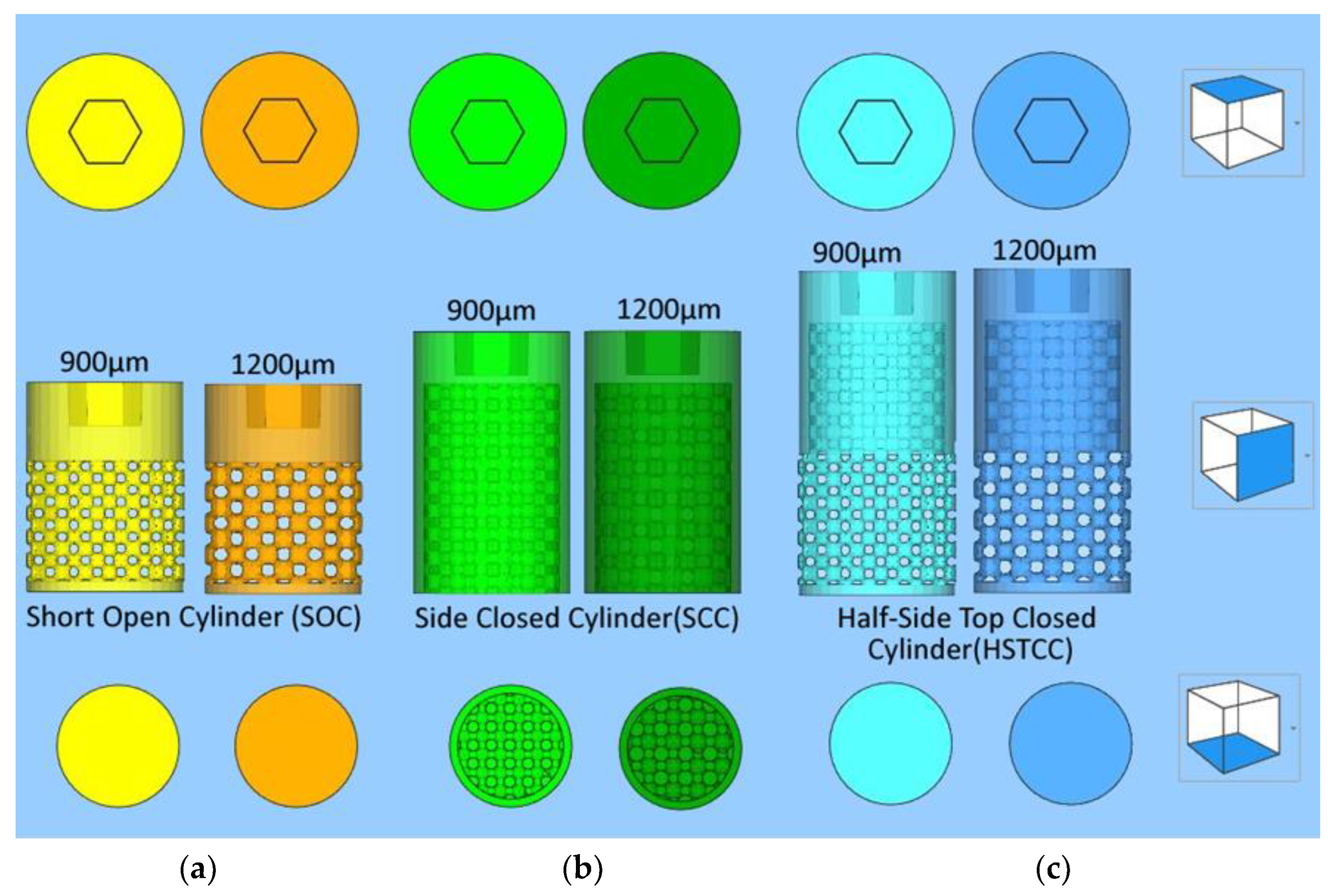
2.1.1. Designs with a Lattice Structure

To study the bone growth in implants including a lattice structure, three different implants were designed (Figure 1) with the characteristics below:

➢

General shape of the three designs: cylinders with a diameter of 6 mm and a top hexagonal hole conceived to accommodate a holder;

➢

Differences between the three different designs:

• Short side-open cylinder: 5 mm of lattices for 8 mm in total height. The top and bottom of the cylinder are closed by dense surfaces. In this way, the bone penetration is peripherally limited (Figure 1a);
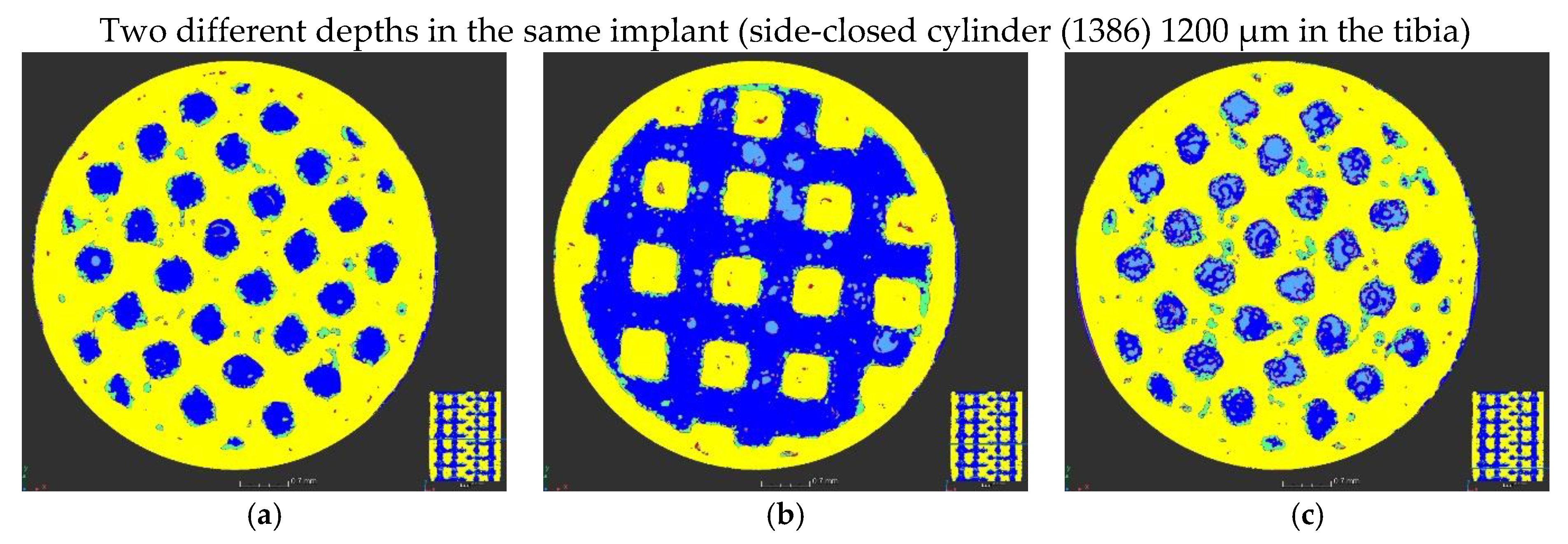
• Side-closed cylinder: 8 mm of lattice for 10 mm in total height The bottom of the cylinder is open. In this way, the bone penetration is bottom limited (Figure 1b).
• Half-side-closed cylinder: 10.4 mm of lattice for 12.4 mm in total. The top and bottom of the cylinder are closed by dense surfaces. In this way, the bone penetration is half peripherally limited (Figure 1c);

➢

Ø Shape of the elementary cells of the lattice: cubic octahedron (diagonal cell);

➢

Ø Size of the elementary cells of the lattice: 900 µm (octahedron with diagonal cell size of 350 µm) or 1200 µm (octahedron with diagonal cell size of 450 µm);

➢

Ø Number of implants studied: five labeled 1382, 1384, 1385, 1387, and 1386 as targeted in Figure 1.

2.1.2. Manufacturing in a New Titanium Alloy Using a Powder Bed Fusion-Laser Beam (PBF-LB) Process

The implants (Figure 2) were additively manufactured with a laser beam powder bed fusion (PBF-LB) process by Z3Dlab using the patented titanium alloy Ti–19Nb–14Zr (at %), hereinafter ZTM14N [7]. The pre-alloyed powder of Ti–19Nb–14Zr (at %) was produced using powder atomization to obtain a spherical-shaped powder. An SLM 125HL (SLM solution) PBF-LB machine equipped with a 200 W ytterbium fiber laser was employed. The layer thickness was chosen to be 30 µm, and the temperature of the building platform was kept constant at 200 °C to minimize residual stresses.

None of these samples underwent heat treatment or polishing. However, the following cleaning protocol was applied:

(1)

60 min in an ultrasound tank with 60 °C distilled water without any detergent;

(2)

30 min soaking in Dentasept 3 H rapid for decontamination;

(3)

Rinsing by ultrasound;

(4)

Cleaning with benzalkonium chloride, chloramine T, E.D.T.A betatetrasodium, and isopropylic alcohol;

(5)

Drying at DPH21;

(6)

Sterilization by surgical autoclave.

At the end, the bulk density and density of the implant were measured with a He-pycnometer and are, respectively, 99.95% ± 0.05% and 5.54 g/cm³.

2.2. Animal

2.2.1. Animal Model

Two female sheep were involved in this study, which was performed in accordance with good laboratory practices. The sheep were bred by the French National Research Institute for Agriculture, Food and Environment (Institut national de recherche pour l’agriculture, l’alimentation et l’environnement (INRAE)). The animals’ ages ranged between five and a half and six years, and their weights were around 55 kg. Tibias and metatarsal bones were used for the inclusion of all implants. For two days immediately following implant placement surgery, the two sheep were housed in individual pens with eye contact. Then, they were housed in a paddock with a group of sheep until the implant removal surgery. In this paddock, the temperature was maintained between 19 °C and 22 °C, the sheep were exposed to an artificial 12 L–12 G light cycle, they were supplied with vegetal bedding, and fed with hay and water ad libitum. A daily check of their physical condition was performed throughout the study.

2.2.2. Surgical Steps of the Implant Placement

The surgical operations (Figure 3a) enabling the placement and removal of the implants into and from the sheep were approved by the French Ministry of Research after ethical evaluation by the facility’s Ethical Committee. These operations were performed by a surgeon assisted by a technician at the Biomedical Research Center of the National Veterinary School of Alfort in France (Centre de Recherche BioMédicale (CRBM) de l’Ecole Nationale Vétérinaire d’Alfort). The center has a dedicated operating room for both large and small animals. Prior to the operation, the sheep underwent a complete veterinary examination and then anesthesia. The anesthetic and analgesic protocol performed by an anesthetist implied the following steps:

(1)

Pre-medication by intravenous injection of a mixture of ketamine (6 mg/kg) and diazepam (0.5 mg/kg);

(2)

Intubation with an endo-tracheal probe of 9 mm internal diameter;

(3)

Connection to respirator with maintenance of anesthesia by inhalation of 2.5% isoflurane in an air/oxygen mixture with 60% O₂;

(4)

Analgesia: IV injection of morphine (0.1 mg/kg);

(5)

NSAIDs: IM injection of meloxicam (0.4 mg/kg);

(6)

Antibiotic: IM injection of 0.15 mL/kg of PeniDHS (combination of penicillin and streptomycin).

After anesthesia, the sheep’s legs were shorn and brushed with chlorhexidine. Then, the cylindrical specimens were placed (Figure 3c) in a bone cavity of the tibias and metatarsal bones, previously drilled at the right dimensions (Figure 3b) by tilting the periosteum, following a strict protocol. Dental implantology equipment was used.

2.2.3. Surgical Steps of the Implant Removal

The euthanasia of the sheep after twelve weeks was performed by pre-medication by intravenous injection of a mixture of ketamine (6 mg/kg) and diazepam (0.5 mg/kg), followed by an injection IV of 20 mL of pentobarbital 18%. For the removal of the implants, the surgical site was taken over by the same approach as the placement surgery. A visual inspection of this surgical site was carried out and compared to the site after the implants’ placement (Figure 4). Then, the bone parts including the cylindrical specimens were sliced and immediately frozen at −18 °C. Finally, the parts were transferred in dry ice to BAM in Berlin, where they were kept frozen at −18 °C before the XCT characterizations.

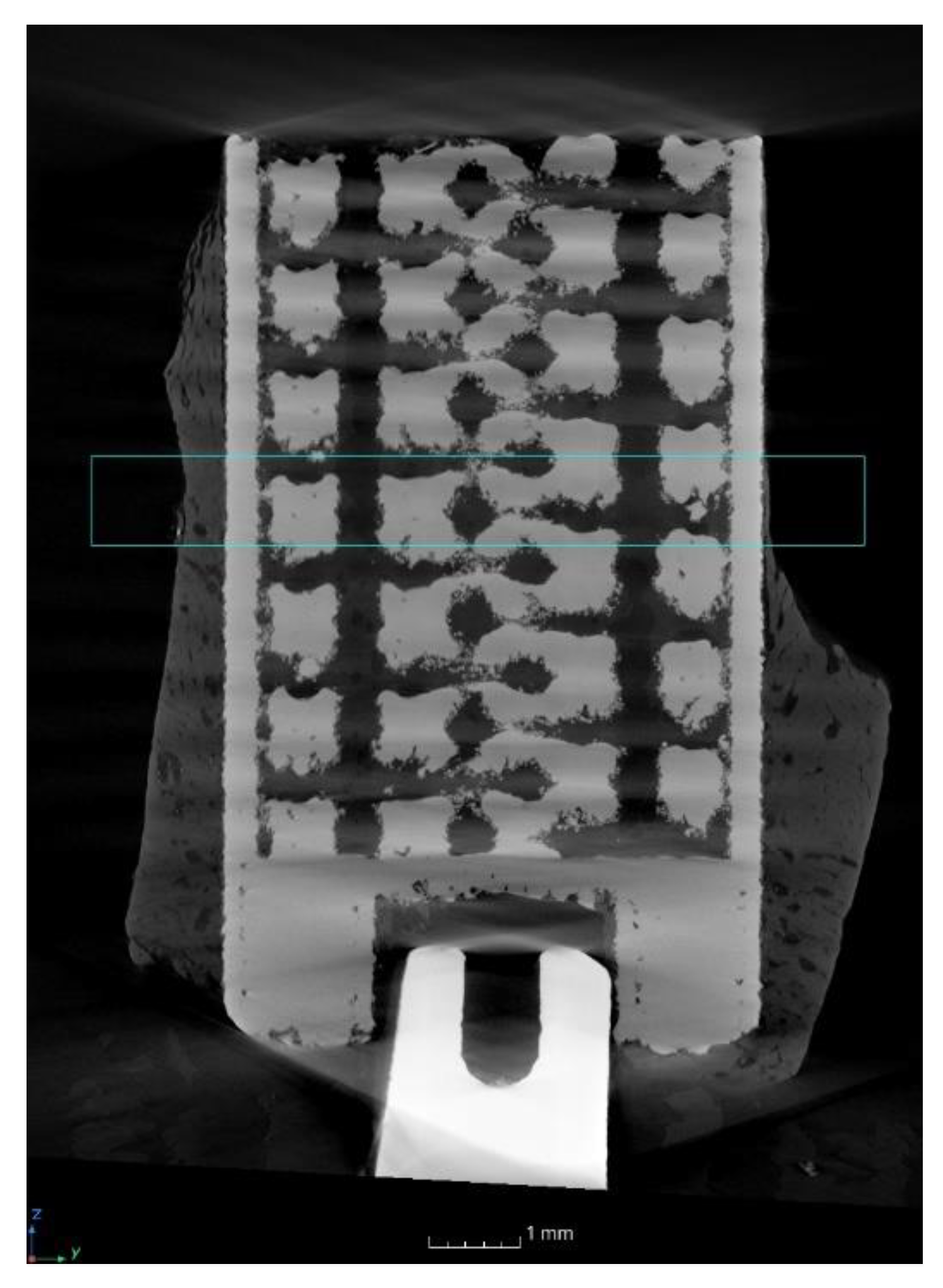
2.3. Characterization of the Implant Using an X-ray Computed Tomography (XCT) System

X-ray computed tomography (XCT) imaging was conducted at BAM with an industrial General Electric (GE) phoenix v|tome|x L 300/180 cone–beam XCT system. This system includes a 300 kV microfocus X-ray tube, as well as a 180 kV high-resolution nanofocus X-ray tube. The entire system is mounted on a granite-base 8-axes manipulator. The 180 kV high-resolution nanofocus X-ray tube was used for the scanning of the implants. This tube includes a transmission target made of tungsten on diamond with a minimum focal spot size of 1 μm. The custom bay system is also equipped with a GE 2048 × 2048 pixel (200 μm pitch) 14-bit amorphous silicon flat panel detector. The acquisitions (version datos|x 2.2.1.695) and the reconstruction (version datos|x 2.1.0.582—RTM) after the scans were performed with the phoenix datos|x GE software (version number 2.2.1.695).

A photo of the set-up is shown in Figure 5. The samples were removed from the freezer just before the acquisitions and returned to the freezer immediately after the acquisitions. They were not maintained at −18 °C during the acquisitions. The XCT parameters used are provided in

Table 1. XCT acquisition parameters used for the implant characterizations.

Accelerating Voltage (kV)	Current (µA)	Number of Projection	Exposure Time per Projection (ms)	Number of Projection Averaged	Scan Duration (h)	Voxel Size (µm)
120	120	3142	1000	2	2	6.8

. No filter was used. A geometrical magnification of 30 was achieved by positioning the samples close to the beam X-ray source (Figure 5a), giving an effective voxel size of 6.8 μm.

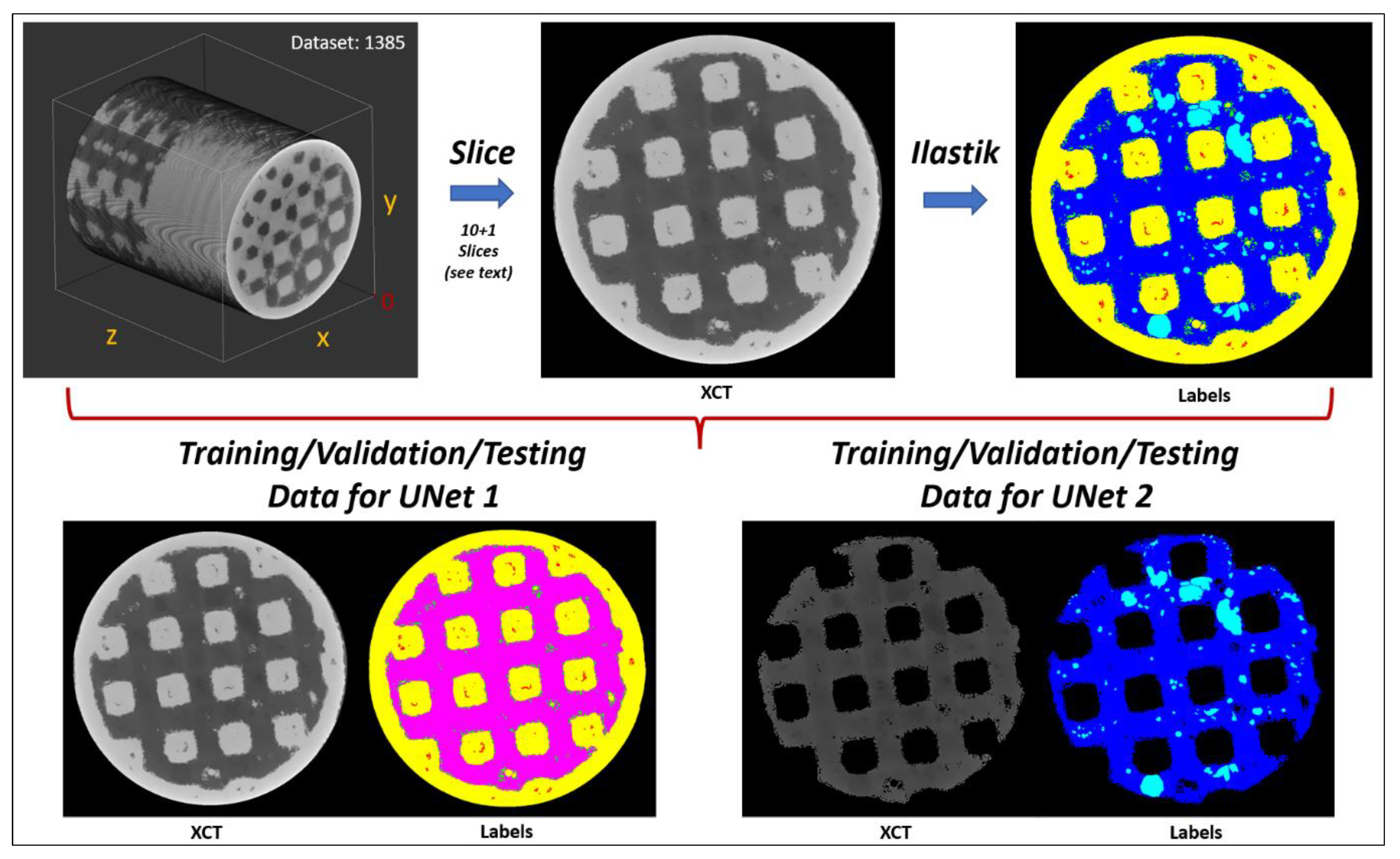
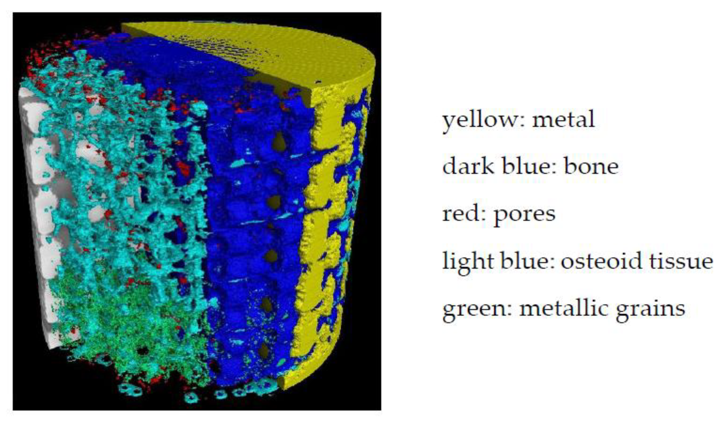
2.4. Analysis of the XCT Images Implementing a Machine Learning (ML) Segmentation

The separation of the metal, bone, pores, osteoid tissue, and metallic grains from each other on the 3D images was carried out with the Ilastik program [15] and two custom in-house 2D UNets [16], forming a three-stage sequential ML process. Ilastik was used to annotate/generate efficiently the training data, which were subsequently employed to train the UNets. This approach reduced considerably the time required to annotate the training labels compared to purely manual annotation. In other words, we accelerated the annotation of the required (by the UNets) training labels with the ML capabilities of Ilastik.

Ilastik has been developed by the Ilastik team in Anna Kreshuk’s laboratory at the European Molecular Biology Laboratory (EMBL) in Heidelberg (Germany), and uses iterative ML algorithms to segment, classify, track, and count the different image areas in 2D images and 3D stacks.

The pixel classification workflow in Ilastik assigns pixels to a group based on pixel/voxel features. These features can be selected by the user from a wide range of operations, for example, smoothed pixel/voxel intensity, edge filters, and texture descriptors. The user then selects some representative areas in the 3D image stack by color-coding the different areas to be segmented. Based on the image areas assigned to the classes by the user, the system interactively trains a random forest classifier. The predictions in the image data can be previewed so that the training can be improved interactively. The result is a unique classification of each pixel/voxel into a previously defined class. These classifications can then be extracted.

The main challenge with these XCT datasets is that it is very difficult to distinguish the bone and osteoid phases from each other based solely on gray values, as they appear very similar. The osteoid phase appears typically slightly darker compared to the bone phase due to its lower density. However, the variation of contrast arising from beam hardening within the XCT datasets can result in certain regions where the bone phase appears darker compared to the osteoid phase located at a different region (i.e., regions in different images within the 3D stack or different locations within the same image). An example of this is shown in Figure 6. The complete segmentation of the datasets with Ilastik could have been possible, but with a lot more (manual) effort to account for all deviations across all regions. Our three-stage ML segmentation method accelerated the whole process by overcoming the above limitations.

Our training strategy was the following:

Firstly, we conditioned the five XCT datasets (labeled: 1382, 1384, 1385, 1386, and 1387) with a non-local-means (NLM) filter [17] (parameters: sigma = 2, smoothing_factor = 1) to reduce noise. Secondly, we extracted from the dataset 1385 eleven random images (4 + 1 along xy plane, 2 along xz plane, and 2 along yz plane, (xy, xz, and yz planes, as shown in Figure 7). Ilastik was employed to annotate the various phases/labels only within these eleven images (metal, bone, pores, osteoid tissue, and metallic grains), which then served as the training/validation/testing data for the UNets. The extra (+1) image from the xy plane was reserved only for testing the final segmentation accuracy (i.e., training/validation: ten image pairs, testing: one image pair). Thirdly, to increase the number of training/validation data, we randomly mirrored/rotated the 10 images to a total of 2000 image pairs (input images and ground truth labels), of which 1800 image pairs (90%) were used as training data, and 200 image pairs (10%) were used as validation data. To improve generalization (i.e., to distinguish the similar bone and osteoid phases better during segmentation), we introduced to the training/validation datasets random brightness and contrast augmentations (+/− 10%) in random order and intensity, moderate random Gaussian noise (0–8 in 8-bit grayscale range: 0–255), and random Gaussian blur (random sigma: 0–1). This approach has been proven by Tsamos et al. [18] to considerably improve the segmentation accuracy of different phases in XCT scans with overlapping gray levels. To further improve the segmentation accuracy, the training of the UNets was undertaken in two stages with a different UNet in each stage. The first UNet was trained to segment the various phases while treating the bone and osteoid phases as a single phase (i.e., 5 phases: metal, pores, metallic grains, bone/osteoid combined, and background). The second UNet was responsible for segmenting only the challenging bone and osteoid phases while considering the rest phases as background (i.e., 3 phases: bone, osteoid, and background). Effectively, the regions in the training/validation image pairs belonging to the metal, pores, and metallic grains phases were nulled (i.e., converted to “black” background) before training the second UNet. Samples of the training/validation/testing data used for the two UNets are illustrated in Figure 7.

The UNet architectures (shown in Figure 8) were designed and trained with Sony’s Neural Network libraries [19] on a workstation equipped with a GeForce RTX 3090 graphics card (Nvidia, Santa Clara, CA, USA), an Intel i7 CPU (Intel, Santa Clara, CA, USA), and 32 GB of memory. The ADAM optimizer [20] was selected as the training algorithm (parameters: initial learning rate/alpha = 10⁻⁴, beta1 = 0.9, beta2 = 0.999, updated every iteration), with an input batch size of 8, and random shuffling for the training dataset on each epoch. The learning rate was updated exponentially on every epoch with a learning rate multiplier LRM = 0.95, and we trained for a total of 300 epochs with Categorical Entropy Loss. The decisive (learnable/trainable) parameters within the UNet architectures were adopted from the epoch that minimized the validation error. Based on the reserved testing image, we report a global accuracy Dice score of 85%.

Our forwarding strategy was the following:

We sliced the NLM-conditioned XCT datasets/stacks in 2D images along all three planes (i.e., xy, xz, and yz planes), and for each plane, we applied four rotations (0°, 90°, 180°, and 270°). Thus, this resulted in 12 different sets of images (12 different views). Each set was forwarded through the first (trained) UNet, resulting in 12 × 5 (5 possible phases for the first UNet) probability map sets. These probability map sets were rotated back to 0° and assembled back into 3D stacks according to the plane direction that was initially sliced, resulting in 12 × 5 probability map 3D stacks. Finally, the probability stacks were summed together according to their respective phase probability group, resulting in 5 probability stacks for the 5 phases. The final classification (i.e., assigned class/label: metal, pores, metallic grains, bone/osteoid combined, or background) was assigned based on the highest phase probability across all 5 probability stacks for each voxel. Based on this segmentation (i.e., from the first UNet), the gray levels of regions (voxels) in the XCT datasets that were segmented/classified as metal, pores, and metallic grains were nulled to appear as background. Next, a similar “multi-view” slicing of these datasets was performed before being fed into the second UNet. The assembly and final classification procedure was exactly the same as in the case of the first UNet (but this time with 3 probability stacks for the 3 phases: bone, osteoid, or background). Finally, we maintained the metal, pores, metallic grains, and background assigned labels from the first UNet segmentation, and the bone and osteoid labels from the second UNet segmentation to compose the concluding segmentation (Figure 9).

2.5. Evaluations of the Osseointegration Process

2.5.1. Bone–Implant Interface (BII) and Bone–Implant Contact (BIC)

The osseointegration process of titanium (Ti) implants in the body begins with the oxidation of Ti on the implant periphery by biological fluids (blood and lymph). This oxidation results in the formation of a TiO₂ layer.

This step is followed by the formation of a calcified (but not ossified) layer with a thickness of about a few nanometers. Such calcification occurs by adsorption on the oxidized metal by the mean of calcium (Ca) and phosphate ions present in the blood. This layer has been observed by Nishikawa et al. [21], Goto [22], and Sundell et al. [23].

Then, healing proceeds by the formation of an intermediate osteoid tissue, the woven or fibrous bone, in the empty spaces. Ossification takes place within this tissue. However, there remains an interface called the bone–interface implant (BII) between the metal and the bone. The surgical success of the integration and fixation of an implanted device in the human body depends on the stability of the implant. This stability is determined by the biomechanical properties of this BII. The BII is the weakest region in the bone–implant system, and most of the failures occur there. Good-quality osseointegration requires close contact between the bone and the implant over a significant proportion of the implant surface. The thickness of this BII is an important characteristic of the quality of osseointegration. A thickness of less than 10 µm is recognized as an indicator of high quality [8,21,24].

The fraction of the implant surface in contact with bone, i.e., the ratio of bone over metal in a given direction, is provided by the bone–implant contact (BIC), a metric that quantifies the stability and the durability of the implant. Classically, the BIC is evaluated by histomorphometry. In the present article, it was evaluated from the XCT images segmented by ML. According to Bernhardt et al. [25] in 2012, histomorphometry and 3D XCT provide similar results. For Lyu et al. [26] in 2011, the BICs evaluated from histomorphometric sections and those evaluated from 2D XCT sections also showed a strong correlation. Finally, Hong et al. [27] in 2022 found the same correlation. Thus, the measurements performed on 2D slices extracted from 3D XCT images are justified.

The advantages of evaluating the BIC from XCT images rather than from histomorphometry are (a) the non-invasive character of XCT, (b) the ability to perform multiple evaluations on different sections (in histomorphometry, the evaluation is performed on thin layers explicitly fabricated), and (c) the 3D approach. Thus, the evaluation of osseointegration of implants from XCT images seems relevant.

In the present study, BICs with the side-closed cylinder open at its bottom were evaluated (8 mm of lattice for 10 mm in total) (Figure 1b). The measurements were performed on 1 mm high sagittal sections (see blue rectangle in Figure 10) corresponding to 150 pixels of 6.8 µm (Figure 11).

More precisely, the sections were located at different angular positions at the cylinder periphery: 0°, 45°, 90° and 135° (Figure 12). On these sections, the number of pixels of osteoid tissue in contact with the metal was counted by visual examination.

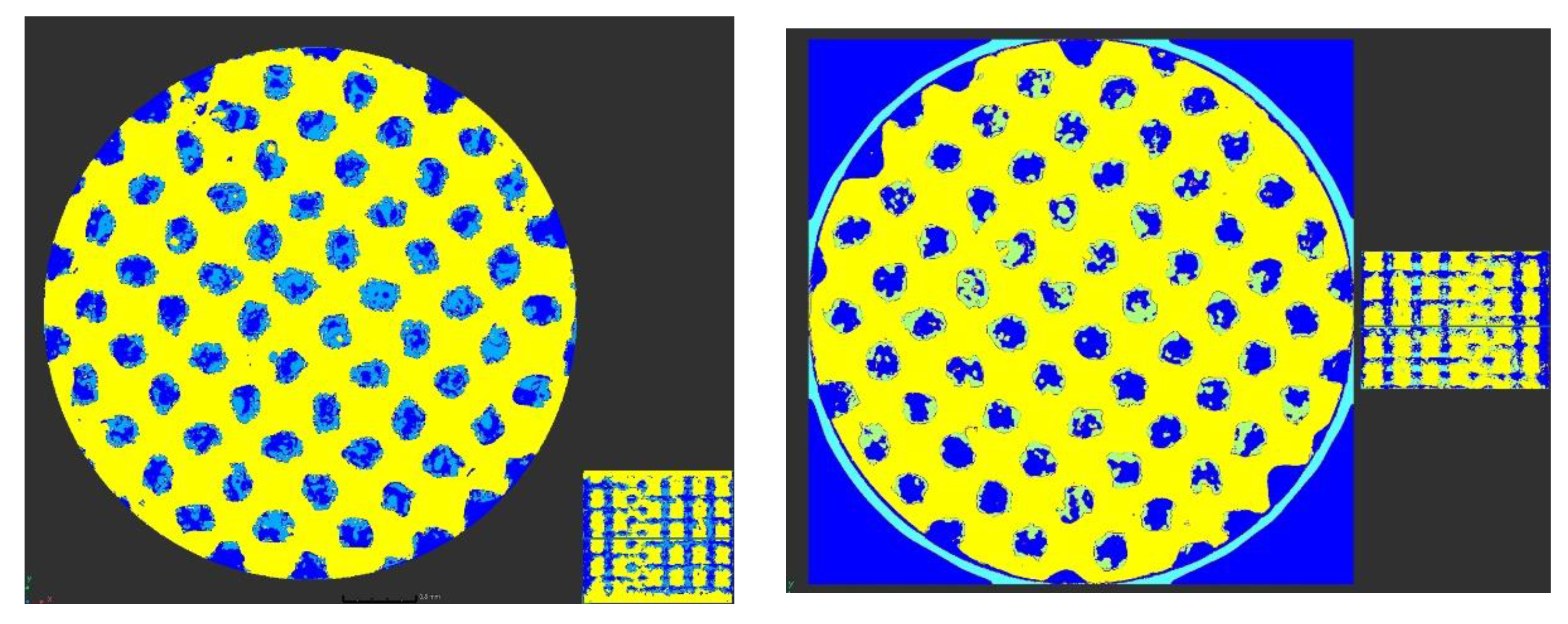
2.5.2. Bone Progression in the Lattice Structure

The bone progression was evaluated from 2D slices and 3D images at the boundary of the metal on the three different designed implants: short-side-open cylinder, side-closed cylinder, and half-side-closed cylinder. Furthermore, to locate the state of bone development, sagittal sections were considered.

3. Results and Discussion Related to the Evaluations of the Osseointegration Process

3.1. Visual Inspection before the Implant Removal

A high overlap of the metal by the bone after twelve weeks can be observed in Figure 4b. According to the surgeon’s experience, this can be attributed to the material’s properties of the new proposed titanium alloy, Ti–19Nb–14Zr, containing Nb and Zr instead of Al and V, and more precisely to the Nb. Indeed, the surgeon who performed the operation did not observe such an overlap with conventional and AM titanium alloys [6].

3.2. BII and BIC

Concerning the BII distance, 10 µm is used as a limit by Nishikawa et al. [21], Jain et al. [24], and the main implant manufacturers of dental implants. In the present study, 1 pixel corresponds to 6.8 µm, which means that the BII is 3.3 µm, much less than 10 µm, thus even more favorable.

The BIC evaluations performed on the four sections displayed in Figure 12 are given in

Table 2. BIC evaluations performed on an area located close to the external border of the side-closed implant, open at its bottom, labeled 1386, for different angular positions at the cylinder periphery.

Angular Position around the Cylinder	0°	45°	90°	135°	Total
Number of pixels in the selected image area	148	151	150	154	603
Number of pixels for which bone and metal have no contact	1	5	17	5	28
% of pixels free of bone or metal	0.6	3.3	11.3	3.2	4.6
BIC (%)	99.4	96.7	88.7	96.8	95.4

. An area located close to the external border of the side-closed implant, open at its bottom, was investigated for different angular positions at the cylinder periphery.

Over the 603 pixels corresponding to the cumulative height of the 4 selected sections on the outer portion of the cylinder, 28 pixels representing bone are not in contact with pixels representing metal, i.e., 4.6%. The contact between the bone and the metal, related to the BIC, is therefore 95.4%. Such a high level of osseointegration promises the highest stability and duration of the implant in the bone. Indeed, classically BICs ranging between 50% and 80% are considered to be favorable scores [28].

A similar count was also performed on the same sections, but on an area located close to the internal border. In this case, the analysis was conducted in the lattice region of the side-closed implant open at its bottom for different angular positions at the cylinder periphery. The results are given in

Table 3. BIC evaluations performed on an area located close to the internal border, in the lattice region of the side-closed implant open at its bottom, labeled 1386, for different angular positions at the cylinder periphery.

Angular Position around the Cylinder	0°	45°	90°	135°	Total
Number of pixels in the selected image area	38	300	254	61	653
Number of pixels for which bone and metal have no contact	0	0	47	0	47
% of pixels free of bone or metal	0	0	18.5	0	7.2
BIC (%)	100	100	81.5	100	92.8

. Out of the 653 pixels considered, 47 did not show bone/implant contact, a rate of 7.1%. The difference in the BIC between the internal and external borders of the implant mainly originates from one of the four considered sections, located at 90°.

The low thickness of the BII and the importance of the BIC may induce stress concentration at the bone–implant junction if there is a high stiffness difference between the bone and the implant. However, in the present study, the smaller difference between Young’s modulus, i.e., the metric representing the stiffness of the cortical bone (25–30 GPa) and the new used alloy (38 GPa), has reduced the effective stress compared to other commonly used materials.

3.3. Bone Progression in Lattice Structures

First of all, the bone progression was examined as a function of the location of the implants in the sheep’s body, i.e., the bone progression in the metatarsal bone was compared to that in the tibia (Figure 13). The percentages of bone (dark blue in Figure 13) and of osteoid tissue (light blue in Figure 13) within the lattice are, respectively, 20.5% and 8.8% for the metatarsal bone and 26.6% and 3.9% for the tibia for the same sheep. Therefore, it seems that the bone progression is more accentuated in the tibia than in the metatarsal bone. This result confirms that vascularization, one of the four processes that come into play in implant stabilization, is better in the tibia than in the metatarsal bone.

Then, the bone progression was examined as a function of the type of designs of the implants (Figure 14), as a function of the depths in the implants (Figure 15), and as a function of the lattice cell sizes (Figure 16). At 5 mm depth, the bone formation is almost complete for the 1200 µm lattice cell size, whatever the implant design (Figure 14b,c and Figure 15a,b). At 8 mm, the bone creation is not complete when the cylinder is laterally closed at all its height for the 1200 µm lattice cell size (compare Figure 15b with Figure 15c). For the 900 µm lattice cell size, bone creation exists but seems incomplete (Figure 14c and Figure 16). However, it is not possible to conclude from this study whether the size of the lattice cell or its location in the sheep’s body is the cause of this incomplete ossification.

4. Conclusions

Additive manufacturing naturally leads to a high-roughness surface finish. This roughness has a positive effect, as it increases the wettability of the implant. Furthermore, the new proposed titanium alloy, Ti–19Nb–14Zr, has an increased affinity to bone, which enhances the quality of osseointegration. At last, the lattice provides crevices in which the biological tissue can jump in and cling. The combination of these factors is pushing ossification beyond its natural limits.

In France in 2017, 19,000 patients had to undergo further surgery for unsealing their prostheses. Thus, the stabilization of hip prosthesis needs to be increased, but in anticipation of the need for its removal, the procedure must be simplified by a bone spline key that can be easily cut for prosthesis removal. Bone spline key has been already investigated in dental implants by tunneling their apex into the bone (e.g., Paragon implant). However, the insufficient ossification of this transfixing cavity has led to a disaffection of this technique. The type of laterally closed lattice structures described in this article allows this technique to be reconsidered.

The speed and quality through high stability of the osseointegration of an implant into a patient’s body is crucial for the rapid recovery of the patient, as well as the durability of prosthesis implantation for a better quality of life. The new titanium alloy (Ti–19Nb–14Zr) proposed in this paper increases the quality of osseointegration with a BIC of 95% and speeds up the ossification compared to conventionally used titanium alloys. In addition, the lattice structure of the implant increases its stability, and the lateral closing up of the lattice structures opens the possibility for bone spline key of prostheses allowing the implant to be removed more easily if required (end of life of the implant, material incompatibility into the body, bad positioning). Thus, this new titanium alloy, whose flexibility is close to that of the cortical bone, reduces stress at the bone/implant junction and hence the risk of loosening, and such laterally closed lattice structures are appropriate candidates to be implemented in a new generation of implants. This new generation of implants is made necessary to face the medical complications that can arise with certain components in alloys presently used, such as Al and V, as well as the prohibition of cobalt in 2025, decreed by the European Chemicals Agency (ECHA) in 2017, and included and enshrined in the European regulation [29]. The next step of this study, consisting of establishing a partnership with the medical sector to implement a comparative study of the available implants on the market and our proposal (material and geometrical configuration), is ongoing to demonstrate its value. A statistical study will be included.

References

1. Abbas, M.M.; Rasheed, M. Solid State Reaction Synthesis and Characterization of Cu doped TiO2 Nanomaterials. J. Phys. Conf. Ser. 2020, 1795, 012059. [Google Scholar] [CrossRef]
2. Alshalal, I.; Al-Zuhairi, I.H.-M.; Awad Abtan, A.; Rasheed, M.; Khalil Asmail, M. Characterization of wear and fatigue behavior of aluminum piston alloy using alumina nanoparticles. J. Mech. Behav. Biomed. Mater. 2023, 32, 20220280. [Google Scholar] [CrossRef]
3. Khorasani, M.; Ghasemi, A.-H.; Leary, M.; Downing, D.; Gibson, I.; Sharabian, E.G.; Kozhuthala, V.-J.; Brandt, M.; Bateman, S.; Rolfe, B. Benchmark models for conduction and keyhole modes in laser-based powder bed fusion of Inconel 718. Opt. Laser Technol. 2023, 164, 109509. [Google Scholar] [CrossRef]
4. Huang, X.; Ding, S.; Lang, L.; Gong, S. Compressive response of selective laser-melted lattice structures with different strut sizes based on theoretical, numerical and experimental approaches. Rapid Prototyp. J. 2023, 29, 209–217. [Google Scholar] [CrossRef]
5. Yue, M.; Li, M.; An, N.; Yang, K.; Wang, J.; Zhou, J. Modeling SEBM process of tantalum lattices. Rapid Prototyp. J. 2023, 29, 232–245. [Google Scholar] [CrossRef]
6. Obaton, A.-F.; Fain, J.; Djemaï, M.; Meinel, D.; Léonard, F.; Mahé, E.; Lécuelle, B.; Fouchet, J.-J.; Bruno, G. In vivo XCT bone characterization of lattice structured implants fabricated by additive manufacturing: A case report. Heliyon 2017, 3, e00374. [Google Scholar] [CrossRef] [Green Version]
7. Djemai, A.; Fouchet, J.-J. Process for Manufacturing a Titanium Niobium Zirconium (tnz) Beta-Alloy with a Very Low Modulus of Elasticity for Biomedical Applications and Method for Productive Same by Additive Manufacturing. WO2017137671A1, 17 August 2017. [Google Scholar]
8. ASTM WK84537; New Specification for Additive Manufacturing—Finished Part Properties—Titanium-27Niobium-21Zirconium via Laser Beam Powder Bed Fusion for Medical Implant Applications. ASTM: West Conshohocken, PA, USA, 2022.
9. Boyer, R.; Collings, E.W.; Welsch, G. Materials Properties Handbook: Titanium Alloys; ASM International: Almere, The Netherlands, 1994. [Google Scholar]
10. Lee, D.-G.; Mi, X.; Eom, T.K.; Lee, Y. Bio-Compatible Properties of Ti–Nb–Zr Titanium Alloy with Extra Low Modulus. J. Biomater. Tissue Eng. 2016, 6, 798–801. [Google Scholar] [CrossRef]
11. Kurtz, M.; Wessinger, A.; Mace, A.; Moreno-Reyes, A.; Gilbert, J. Corrosion Resistance of Additively Manufactured Titanium Alloys in Physiological and Inflammatory-Simulating Environments: Ti-6Al-4v Versus Ti-29Nb-21zr. Mater. Eng. 2022. [Google Scholar] [CrossRef]
12. Kurtz, M.; Wessinger, A.; Mace, A.; Moreno-Reyes, A.; Gilbert, J. Additively manufactured Ti-29Nb-21Zr shows improved oxide polarization resistance versus Ti-6Al-4V in inflammatory stimulating solution. J. Biomed. Mater. Res. 2023, 1–16. [Google Scholar]
13. Walker, P.R.; LeBlanc, J.; Sikorska, M. Effects of aluminum and other cations on the structure of brain and liver chromatin. Biochemistry 1989, 28, 3911–3915. [Google Scholar] [CrossRef] [PubMed]
14. Rao, S.; Ushida, T.; Tateishi, T.; Okazaki, Y.; Asao, S. Effect of Ti, Al, and V ions on the relative growth rate of fibroblasts (L929) and osteoblasts (MC3T3-E1) cells. Biomed. Mater. Eng. 1996, 6, 79–86. [Google Scholar] [CrossRef] [PubMed]
15. Berg, S.; Kutra, D.; Kroeger, T.; Straehle, C.N.; Kausler, B.X.; Haubold, C.; Schiegg, M.; Ales, J.; Beier, T.; Rudy, M.; et al. Ilastik: Interactive machine learning for (bio)image analysis. Nat. Methods 2019, 16, 1226–1232. [Google Scholar] [CrossRef] [PubMed]
16. Ronneberger, O.; Fischer, P.; Brox, T. U-Net: Convolutional Networks for Biomedical Image Segmentation, Lecture Notes in Computer Science; Springer International Publishing: Cham, Switzerland, 2015; Volume 9351, pp. 234–241. [Google Scholar] [CrossRef] [Green Version]
17. Buades, A.B.; Coll, J.-M.; Morel, A. Non-Local Algorithm for Image Denoising. In Proceedings of the IEEE Computer Society Conference on Computer Vision and Pattern Recognition (CVPR’05), San Diego, CA, USA, 20–25 June 2005; Volume 2, pp. 60–65. [Google Scholar]
18. Tsamos, A.; Evsevleev, S.; Fioresi, R.; Faglioni, F.; Bruno, G. Synthetic data generation for automatic segmentation of X-ray computed tomography reconstructions of complex microstructures. J. Imaging 2023, 9, 22. [Google Scholar] [CrossRef] [PubMed]
19. Neural Network Libraries. An Open-Source Software to Make Research, Development and Implementation of Neural Network More Efficient. Sony Corp. Available online: https://nnabla.org/ (accessed on 9 January 2022).
20. Kingma, D.P.; Ba, J. Adam: A Method for Stochastic Optimization, ICLR 2015. Available online: https://www.semanticscholar.org/paper/a6cb366736791bcccc5c8639de5a8f9636bf87e8 (accessed on 9 January 2022).
21. Nishikawa, T.; Masuno, K.; Mori, M.; Tajine, Y.; Kakudo, K.; Tanaka, A. Calcification at the interface between titanium implants and bone observation with confocal laser scanning microscopy. J. Oral. Implantol. 2006, 32, 211–217. [Google Scholar] [CrossRef]
22. Goto, T. Ostéointégration and dentals implants. Clin. Calcium 2014, 24, 265–271. Available online: https://pubmed.ncbi.nlm.nih.gov/24473360/ (accessed on 10 May 2023).
23. Sundell, G.; Dahlin, C.; Andersson, M.; Thuvander, M. The bone implant interface of dentals implants in humans on the atomic scale. Acta Biomater. 2017, 48, 445–450. [Google Scholar] [CrossRef]
24. Jain, R.; Kapour, D. The dynamic interface: A review. J. Int. Soc. Prev. Commun. Dent 2015, 5, 354–358. [Google Scholar] [CrossRef] [Green Version]
25. Bernhardt, R.; Kublisch, E.; Schultz, M.-C.; Eckelt, U.; Stadlinger, B. Comparison of bone-implant contact and bone-implant volume between 2D-histological sections and 3D-SRµCT slices. Eur. Cell Mater. 2012, 23, 237–247. [Google Scholar] [CrossRef]
26. Lyu, H.-Z.; Lee, J.H. Correlation between two-dimensional micro-CT and histomorphometry for assessment of the implant osseointegration in rabbit tibia model. Biomater. Res. 2011, 25, 11. [Google Scholar] [CrossRef]
27. Hong, J.-M.; Kim, H.-G.; Luke Yeo, I.-S. Comparison of three-dimensional digital analysis and the two-dimensional histomorphometric analysis of the bone-implant interface. PLoS ONE 2022, 17, e276269. [Google Scholar] [CrossRef]
28. Lian, Z.; Guan, H.; Ivanovski, S.; Loo, Y.-C.; Johnson, N.-W.; Zhang, H. Effect of bone to implant percentage on bone remodeling surrounding a dental implant. Int. J. Oral Maxillofac. Surg. 2010, 39, 690–698. [Google Scholar] [CrossRef] [PubMed] [Green Version]
29. Regulation (EU) 2020/561 of the European Parliament and of the Council of 23 April 2020 Amending Regulation (EU) 2017/745 on Medical Devices, as Regards the Dates of Application of Certain of Its Provisions (Text with EEA Relevance), Document 32020R0561. Available online: http://data.europa.eu/eli/reg/2020/561/oj (accessed on 6 May 2023).
Figure 1. The three different designs of the implants with a lattice structure (“meta” stands for metatarsal bone): (a) 1382:900 µm, meta, 1384:900 µm, tibia; (b) 1386:1200 µm, tibia; (c) 1385:1200 µm, tibia, 1387:900 µm, meta.
Applsci 13 07282 g001
Figure 2. Titanium alloy manufactured implants with a lattice structure (three different designs).
Applsci 13 07282 g002
Figure 3. Surgical steps of the implant placement: (a) surgical operating room; (b) drilling of the bone for implant placement; (c) implant placement.
Applsci 13 07282 g003
Figure 4. Comparison of the surgical sites: (a) at the end of implant placement; (b) before implant removal after twelve weeks.
Applsci 13 07282 g004
Figure 5. Implant photographs after removal from the sheep and machined for XCT characterization: (a) implant mounted on the XCT system (close to the XCT source in yellow); (b) implant, surrounded by bone, on its holder.
Applsci 13 07282 g005
Figure 6. Bone and osteoid tissue sharing the exact same XCT gray levels at different locations within the same dataset due to beam hardening.
Applsci 13 07282 g006
Figure 7. Training/validation/testing data for the two UNets. Labels: Bone (dark blue), osteoid tissue (light blue), bone and osteoid combined (magenta), pores (red), metal (yellow), metallic grains (green), background (black).
Applsci 13 07282 g007
Figure 8. The two in-house UNet architectures employed for the segmentation.
Applsci 13 07282 g008
Figure 9. Implant 3D XCT image segmentation performed by the Ilastik program implementing machine learning (ML) algorithms.
Applsci 13 07282 g009
Figure 10. Two-dimensional (2D) XCT sagittal slice of the side-closed implant, open at its bottom, labeled 1386. The blue rectangle is indicating the sections where the BICs were evaluated.
Applsci 13 07282 g010
Figure 11. Grayscale, as well as colored, ML segmented 2D XCT slices of the side-closed implant (labeled 1386), open at its bottom. The inserts are indicating the location where the BICs were measured.
Applsci 13 07282 g011
Figure 12. ML segmented 2D XCT image sections, located at different angular positions at the cylinder periphery, used to evaluate the BICs of the side-closed implant, open at its bottom, labeled 1386: (a) 0°; (b) 45°; (c) 90°; (d) 135°.
Applsci 13 07282 g012
Figure 13. Two-dimensional (2D) XCT images of implant horizontal (top) and sagittal (bottom) slices showing the proportion of bone (in dark blue) within the implant (in yellow) compared to other areas (osteoid tissue is in light blue and metallic grains are in green), in the metatarsal bone and tibia. The green or red line in the smaller images located on the right of the main images indicate where the slices were extracted.
Applsci 13 07282 g013aApplsci 13 07282 g013b
Figure 14. Bone progression in the three types of designs of the implants: (a) Side-open cylinder (1384) 900 µm in the tibia; (b) Half-side-closed cylinder (1385) 1200 µm in the tibia; (c) Side-closed cylinder (1386) 1200 µm in the tibia.
Applsci 13 07282 g014
Figure 15. Bone progression at two different depths in the same implant (Depth 1 = 5 mm and Depth 2 = 8 mm): (a) Depth 1 at the nodes of the lattice’s cells; (b) Depth 1 at the center of the lattice’s cells; (c) Depth 2.
Applsci 13 07282 g015
Figure 16. Bone progression for two different lattice cell sizes of the same implant design: (a) 900 µm (1387, meta); (b) 1200 µm (1385, tibia).
Applsci 13 07282 g016