An Attention-Based CNN-LSTM Method for Effluent Wastewater Quality Prediction

Abstract

Wastewater treatment is a pivotal step in water resource recycling. Predicting effluent wastewater quality can help wastewater treatment plants (WWTPs) establish efficient operations so as to save resources. We propose CNN-LSTM-Attention (CLATT), an attention-based effluent wastewater quality prediction model, which uses a convolutional neural network (CNN) as an encoder and a long short-term memory network (LSTM) as a decoder. An attention mechanism is used to aggregate the information at adjacent sampling times. A sliding window method is proposed to solve the problem of the prediction performance of the model decreasing with time. We conducted the experiment using data collected from a WWTP in Fujian, China. Our results show that the accuracy of prediction is improved, with MSE decreasing by 0.25, MAPE decreasing by 5% and LER decreasing by 7%, after using the sliding window method. Compared with other methods, CLATT achieves the fastest prediction speed among all the methods based on LSTM and the most accurate prediction performance, with MSE increasing up to 0.92, MAPE up to 0.08 and LER up to 0.11. Furthermore, we performed an ablation study on the proposed method to validate the rationality of the major part of the model, and the results show that the LSTM significantly improves the predictive performance of the model, and the CNN and the attention mechanism also improve the accuracy of the prediction.

1. Introduction

Wastewater treatment, which refers to the use of physical, chemical and biological methods to treat wastewater, can reduce pollution and make full use of water resources. Wastewater treatment plants (WWTPs) play a significant role in water resource recycling, allowing the treated wastewater to be discharged directly or reused.

In order to protect the environment, WWTPs need to meet the requirements of local regulations [1]. WWTPs use sensors to obtain effluent wastewater quality indicators and regulate the treatment process according to these indicators; this approach creates hysteresis in the control method and makes it difficult to establish effective control methods for WWTPs. Therefore, most WWTPs make use of excessive control methods, which means the wastewater plants can meet the requirements by adding excessive chemicals, taking over aeration, etc. This measure not only wastes a lot of resources, but also fails to keep WWTPs operating efficiently. If we can predict the quality of effluent wastewater when it flows in, WWTPs can establish effective control methods instead of excessive control methods to save energy and prevent wastewater quality indicators from exceeding the standard.

Predicting effluent wastewater quality via modeling simulates the complicated and dynamic process of wastewater treatment, in which many unmeasured biochemical reactions occur. Each biochemical reaction consumes existing substances and produces new substances. The theory of wastewater treatment can explain some of the biochemical reactions; moreover, the model methods based on the reaction mechanism, such as the Activated Sludge Model (ASM) [2,3], use differential equations to model the dynamic process of wastewater treatment, and their predictive reliability has been verified in practice [4,5]. However, this kind of method needs to determine a large number of parameters, and these parameters need to be updated with changes in time and working conditions to ensure the accuracy of the prediction. This process of updating parameters requires a lot of manpower and material resources.

The rate of biochemical reaction in wastewater treatment will vary with changes in wastewater components, process control settings and weather conditions. Many factors are coupled with each other, which makes the whole wastewater treatment process a complex nonlinear system. Data-driven neural network methods have the powerful capability of modeling nonlinear processes and have been successfully applied in many fields. Compared with model methods based on reaction mechanisms, the neural network method does not require too much mathematical derivation and calculation. It can automatically select the important characteristics of wastewater quality and establish nonlinear relationships to predict effluent wastewater quality according to these characteristics by learning.

Pakrou et al. [6] applied artificial neural networks to predict the wastewater chemical oxygen demand (COD) concentration of treated water in treatment plants. They identified the best model by combining several input variables. Nourani et al. [7] applied a neural network ensemble and other machine learning methods to predict effluent biological oxygen demand (BOD), COD and total nitrogen (TN). The results show that the NNE model is a more robust and reliable ensemble method for predicting WWTP performance due to its non-linear averaging kernel. Dong et al. [8] used random forest (RF) models, and deep neural network (DNN) models to predict the total suspended solids (TSS) and phosphate in effluent. Zhang et al. [9] proposed a convolutional neural network (CNN) model called Reg-CNN to predict wastewater quality containing COD, total phosphorus (TP), ammonia nitrogen (NH3-N) and pH; the results show that Reg-CNN achieves better prediction results than other machine learning methods. Li et al. [10] proposed a novel hybrid CLSTMA method and compared CLSTMA with CLSTM; the results shows that CLSTMA is more accurate than CLSTM in predicting performance. R. Jafar et al. [11] applied a CNN, a recurrent neural network (RNN) and other machine learning methods to predict the effluent concentrations of several wastewater quality indicators (COD, BOD, etc.); the authors attribute the poor prediction result to the small datasets. WAN et al. [12] improved long short-term memory networks (LSTM) by combining the oblivion gate and the input gate into a new input gate, adding a peephole and integrating the Gaussian regression algorithm to achieve the prediction of the COD and suspended matter of the effluent. Wang et al. [13] proposed a long short-term memory network water quality prediction model (SSAA-LSTM) based on SSA and an attention mechanism to predict the COD. Existing data-driven neural network methods are based on a single neural network model to predict effluent wastewater quality.

The existing methods have achieved significant performance in the prediction of effluent wastewater quality, but there are still some problems to be tackled:

First and foremost, the existing neural network methods mostly adopt a single neural network structure for prediction, and have weak nonlinear modeling ability, making it difficult to model the complex biochemical process of wastewater treatment. Second, wastewater treatment is a continuous flow and mixing process; wastewater quality data collected at adjacent sampling times have a strong correlation, and effluent wastewater quality information from the previous moment should also be fully applied to predict effluent wastewater quality. Finally, in its actual production, wastewater will continuously pour into WWTPs; wastewater quality condition is in flux, and the prediction method should have the ability to update dynamically.

We propose a CNN-LSTM-Attention hybrid model called CLATT in combination with the sliding window method to predict the quality of effluent wastewater. A CNN [14,15] can capture local patterns of time series data, such as trends, while an LSTM [16] can integrate these patterns into long-term dependencies. The proposed method improves nonlinear modeling ability by establishing a CNN-LSTM hybrid model. In addition, an attention mechanism is used to integrate the output of the LSTM at adjacent sampling times and extract the information from previous moments. In this paper, a sliding window method is also proposed. By dividing the original prediction method into multi-step prediction, the internal parameters of the model can be dynamically updated with time, enabling it to meet the actual production demand of WWTPs. Extensive experimental results show that our method is more accurate than other deep neural networks. Briefly, our main contributions are:

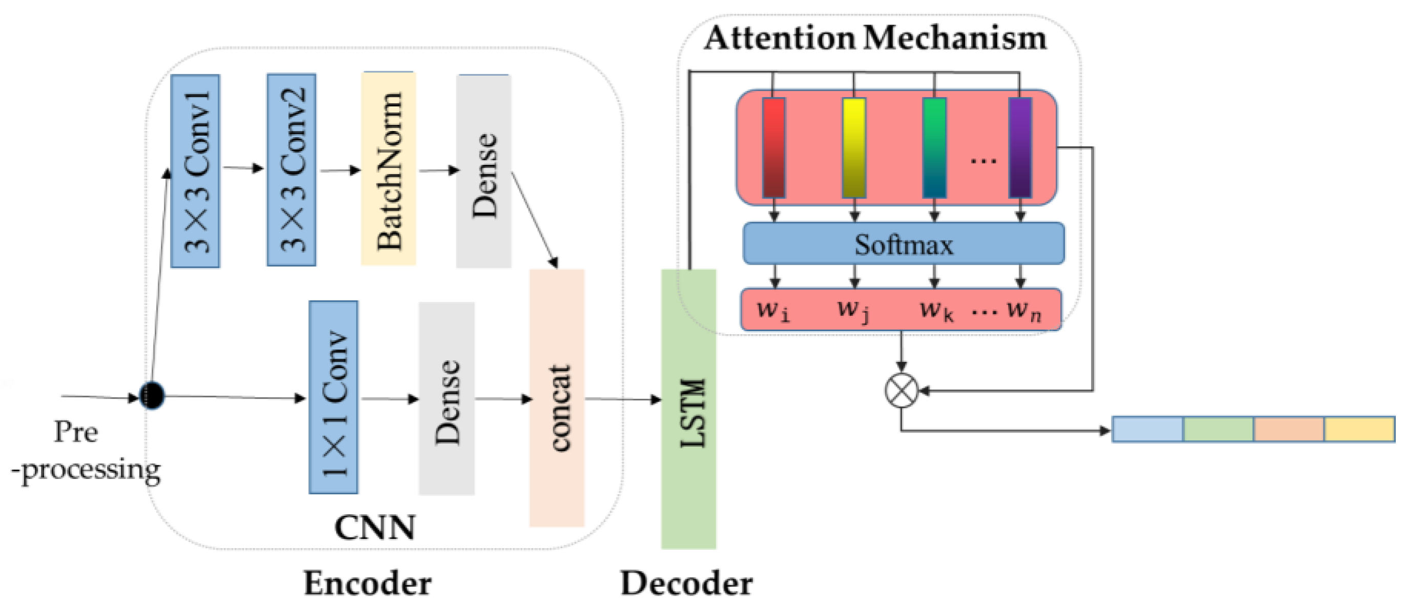
• A hybrid model for effluent wastewater quality prediction that uses a CNN as an encoder and an LSTM as a decoder.
• An attention mechanism to extract the correlation between the wastewater quality data at the adjacent sampling time.
• A sliding window method that supports dynamic updating and can meet the actual use requirements of real-world wastewater treatment plants.

The rest of the paper is arranged as follows:

• Section 2 presents the theoretical background of our method.
• Section 3 introduces the details of the proposed method.
• Section 4 describes the results of the experiments with the corresponding analysis.
• In Section 5, the conclusion is provided.

2. Theoretical Background

2.1. Convolutional Neural Network

A convolutional neural network (CNN) is a class of feed-forward neural network that includes convolutional computation and has a deep structure. It is one of the representative algorithms of deep learning. A CNN extracts features through convolution operations, in which a small convolution kernel is used to scan the input features. The convolution kernel is a small matrix whose values can be learned or set manually. The convolution kernel moves over the input signal or image and is dotted with a small portion of the feature map at each position, and the product is added to give a single value of the output. The output is the response of the convolution kernel at that location, and it represents the feature at that location. The convolution operation can be expressed using the following formula:

$$\mathrm{F}\left(\mathrm{x}\right)={\int }_{-\mathrm{\infty }}^{\mathrm{\infty }}\mathrm{f}\left(\mathsf{\tau }\right)\mathrm{g}\left(\mathrm{x}-\mathsf{\tau }\right)\mathrm{d}\mathsf{\tau }$$

(1)

Convolutional neural networks are widely used in many fields, such as image recognition [14,15].

2.2. Long Short-Term Memory

Long short-term memory (LSTM) was proposed in 1997 by Hochreiter and Schmidhuber, who introduced a structure called a “gate” for controlling the flow of information and maintaining long-term memory. The basic structure of LSTM consists of four main gates, including the input gate, forget gate, output gate and cell state. The input and forget gates determine what information should be selected from the current input and the output of the previous time step to be stored in the cell state, while the output gates control what information should be output from the cell state. The cell state is the core component of LSTM, which maintains memory in the network in the long term and updates or clears unnecessary information when necessary.

Long short-term memory has been applied in many fields, such as speech recognition [17], text recognition [18] and machine translation [19], and is also used in various kinds of time series prediction tasks [20,21].

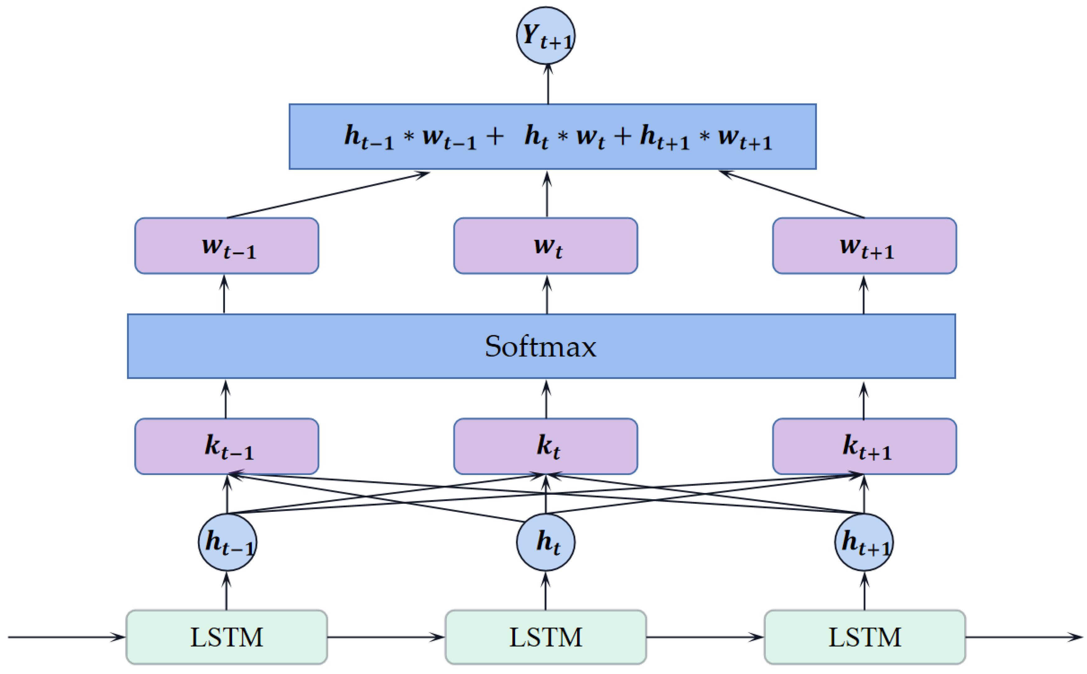
2.3. Attention Mechanism

An attention mechanism [22] refers to how the human visual system automatically selects and focuses attention resources on a specific target while ignoring other irrelevant information when processing visual information. In the field of machine learning, this mechanism is also widely used in neural network models to help improve their accuracy and interpretability when processing complex information.

In neuroscience, researchers have found that the human visual system uses an automated process to sift through information from the outside world to retain important information and ignore irrelevant information. This process is called an attention mechanism. By activating neurons, an attention mechanism filters and focuses visual information to achieve more efficient information processing. In machine learning, we often use attention mechanisms to solve problems. An attention mechanism can solve a problem better by calculating the correlation between different parts to automatically select the parts that need to be dealt with. In computer vision, attention mechanisms are often used to select features of a region or regions and combine these features into a more powerful feature vector for more precise recognition or classification.

3. Proposed Method

CLATT is an encoder–decoder model with an attention mechanism for wastewater quality prediction. The overall structure of the model is shown in Figure 1. In Section 3.1, the preprocessing will be discussed. In Section 3.2, we will focus on the input and output of the model. The encoder-decoder module of the model will be explained in Section 3.3 and the attention mechanism is described in Section 3.4.

3.1. Preprocessing Method

3.1.1. Processing of Abnormal Samples

Our datasets were collected from a wastewater plant in Fujian Province, China. Due to power outages, maintenance or other reasons, there existed vacant or multiple duplicate samples in the datasets, which occurred in about 5 percent of our original datasets. We generated simulated values through interpolation combined with samples at adjacent sampling times, supplemented the vacant samples and replaced the multiple duplicate samples with simulated values. The interpolation formula can be computed as follows:

Y = Y₁ + (X − X₁) (Y₂ − Y₁)/(X₂ − X₁)

(2)

where Y represents the value produced via interpolation, and X stands for the time of interpolation. X₁ and Y₁ represent the value and the time of the previous sampling time. X₂ and Y₂ represent the value and the time of the subsequent sampling time.

The data preprocessing stage also includes the following two methods:

(1)

The distorted data are deleted. The deletion of distorted data is the most common method in data preprocessing. Wastewater quality belongs to a time series, and data at adjacent sampling times have a strong correlation. After deletion, the correlation is damaged, thus increasing the difficulty of prediction. Therefore, the interpolation method is adopted to maintain the correlation between adjacent sampling data.

(2)

The previous sampling data are selected for filling. This method is a commonly used method in real production. When filling multiple continuous data, this method will cause multiple duplicate values, which is one cause of the distorted data we identified. Therefore, the interpolation method is used to prevent the occurrence of multiple duplicate values.

3.1.2. Data Standardization

Since each sample of the datasets contained multiple features and different features were distributed at different orders of magnitude, we needed to normalize the data to ensure that different feature distributions were processed in the same dimension. The normalization formula is as follows:

Z_i = (X_i − μ)/σ

(3)

where Z_i represents the sample value after normalization, and X_i stands for the value of the original sample. μ and σ are the mean and variance of the sample space.

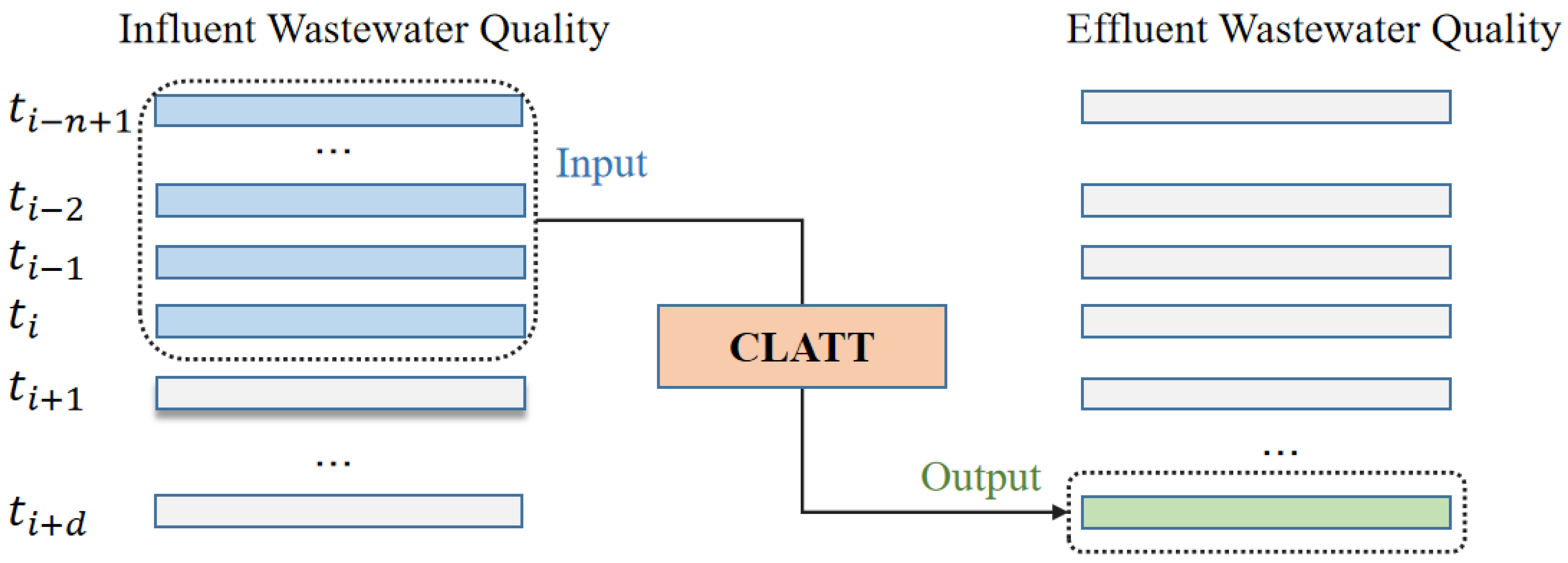
3.2. The Input and Output of the Model

In the actual wastewater treatment process, WWTPs adopt a push-flow design, which removes pollutants through the continuous forward movement of water flow and the reaction with microorganisms. The water flow undergoes a process of constant mixing, and the influent and effluent wastewater quality does not have a strictly one-to-one relationship; that is, when a certain batch of water flows into the WWTP, it is not certain when it will flow out, so we can only estimate the time gap. Consequently, the effluent wastewater quality at one time is affected by the influent wastewater quality several times before.

As shown in Figure 2, the input of the model can be described as below:

$${\mathrm{X}}^{{\mathrm{t}}_{\mathrm{i}}}=({\mathrm{x}}_{{\mathrm{t}}_{\mathrm{i}-\mathrm{n}+1}};{\mathrm{x}}_{{\mathrm{t}}_{\mathrm{i}-\mathrm{n}+2}}{;...;\mathrm{x}}_{{\mathrm{t}}_{\mathrm{i}}})\in {\mathrm{R}}^{\mathrm{n}\times {\mathrm{D}}_{\mathrm{i}\mathrm{n}}}$$

(4)

where ${\mathrm{x}}_{{\mathrm{t}}_{\mathrm{u}}}$ ($\mathrm{i}-\mathrm{n}+1$ ≤ $\mathrm{u}$ ≤ i) refers to the influent water quality measured at ${\mathrm{t}}_{\mathrm{u}}$, and $\mathrm{n}$ represents the input sequence. ${\mathrm{D}}_{\mathrm{i}\mathrm{n}}$ is the number of influent wastewater quality indicators.

Additionally, the corresponding output can be described as below:

$${\mathrm{Y}}^{{\mathrm{t}}_{\mathrm{i}+\mathrm{d}}}\in {\mathrm{R}}^{{\mathrm{D}}_{\mathrm{o}\mathrm{u}\mathrm{t}}}$$

(5)

where ${\mathrm{Y}}^{{\mathrm{t}}_{\mathrm{i}+\mathrm{d}}}$ refers to the effluent wastewater quality measured at ${\mathrm{t}}_{\mathrm{i}+\mathrm{d}}$, and $\mathrm{d}$ refers to the time gap between the inflow and outflow of water from the wastewater treatment plant. ${\mathrm{D}}_{\mathrm{o}\mathrm{u}\mathrm{t}}$ is the number of effluent wastewater quality indicators.

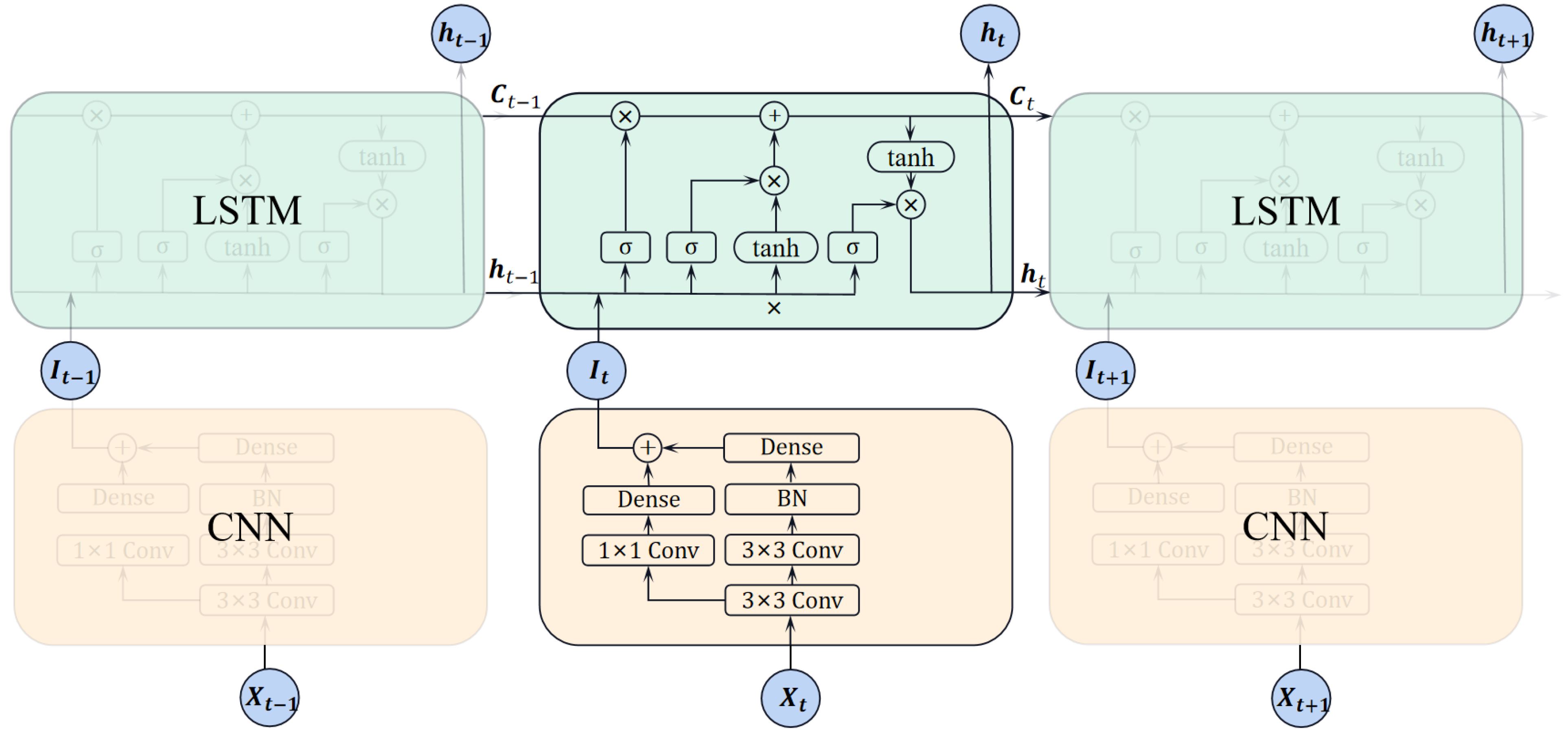
3.3. Encoder–Decoder

As shown in Figure 3, an encoder–decoder structure is adopted in the model that uses a CNN as an encoder and an LSTM as a decoder. The encoder is responsible for converting input into features and the decoder is responsible for converting features into targets.

The encoder is formed by a CNN, such as Resnet [15], which adopts a residual structure to avoid over-fitting. Firstly, since the input contains the time dimension and the feature dimension, two continuous 3 × 3 convolution layers are applied to receive the input and capture feature. After that, it will come through a BatchNormalization (BN) layer, which is widely used to normalize the data to the same quantity and accelerate convergence; then, a Dense layer is used to accept the characteristics and reduce the dimensions, and at the same time, a 1 × 1 convolution layer is used to deliver useful information and concatenate the output of the Dense layer. The concatenated feature is flattened and passes through a Dense layer to reduce the dimensions. The output of the CNN module will be passed to a standard LSTM module as the input. The output of the LSTM module will predict the effluent wastewater quality through the attention mechanism.

3.4. Attention Mechanism

As stated in Section 3.2, WWTPs adopt a push-flow design to flow the wastewater, so the quality of the effluent wastewater at the adjacent sampling time should be highly correlated. As shown in Figure 4, we calculated the PACF (Partial Autocorrelation Function) for four effluent wastewater quality indicators.

In the figure, the zero point of the horizontal axis represents the current time ${\mathrm{t}}_{\mathrm{i}}$, and the remaining points represent the previous times ${\mathrm{t}}_{\mathrm{i}-1},{\mathrm{t}}_{\mathrm{i}-2},\dots {\mathrm{t}}_{\mathrm{i}-\mathrm{n}}$. The vertical axis represents the correlation between the value of the current time and the value of the previous time. The larger the value, the stronger the correlation, and the points outside the blue area represent significant correlation.

As can be seen from the figure above, for the four wastewater quality indicators, the wastewater quality data at the current moment are significantly correlated with the wastewater quality data at the previous two moments. With increasing time, the correlation of the data gradually becomes weaker. To extract the correlation between the wastewater quality data at the current moment and the wastewater quality data at the previous moment, as shown in Figure 5, we propose an attention mechanism for wastewater quality prediction.

Ref. [23] proposed an attention mechanism to aggregates global information. The attention mechanism used in this paper aggregates the information at adjacent moments, and the structure of the attention mechanism is similar to a Dense layer with several weight parameters corresponding to the time dimension of the output from LSTM. The weight is accumulated after being multiplied by the output from LSTM, which produces the predicted effluent water quality. The attention mechanism can be computed as follows:

$${\mathrm{k}}_{\mathrm{i}}=\sum _{\mathrm{t}}\left({\mathrm{h}}_{\mathrm{t}}{\mathrm{h}}_{\mathrm{i}}\right)$$

(6)

$${\mathrm{w}}_{\mathrm{i}}=\exp \left({\mathrm{k}}_{\mathrm{i}}\right)/\exp \left(\sum _{\mathrm{t}}\left({\mathrm{k}}_{\mathrm{t}}\right)\right)$$

(7)

$${\mathrm{Y}}_{\mathrm{t}+1}=\sum _{\mathrm{i}}{\mathrm{w}}_{\mathrm{i}}{\mathrm{h}}_{\mathrm{i}}$$

(8)

where ${\mathrm{h}}_{\mathrm{i}}$ represents the output from LSTM, ${\mathrm{w}}_{\mathrm{i}}$ is the weight of the corresponding output, and ${\mathrm{Y}}_{\mathrm{t}+1}$ refers to the predicted effluent wastewater quality.

4. Experiments

In this section, we will evaluate our method using comparative experiment and describe some of the implementation details. Section 4.1 discusses our datasets. Section 4.2 focus on the baseline and evaluation indicators. The results of the experiments and an ablation study on the model’s parts is described in Section 4.3.

4.1. Datasets

Our dataset, called WD-1, was collected from a wastewater plant in Fujian Province, China, which runs stably and samples every two hours. WD-1 contained 2622 samples collected from 30 May 2022 to 1 February 2023. The dataset was divided into a training set with 2102 samples, a validation set with 20 samples and a test set with 500 samples, and all the samples had six inputs and four effluent wastewater quality indicators, as shown in

Table 1. Influent and effluent wastewater quality indicators.

Indicators
Influent	Chemical Oxygen Demand (COD)
	Ammonia Nitrogen (NH3-N)
	Total Phosphorus (TP)
	Total Nitrogen (TN) Water Flow Rate
	PH
Effluent	COD
	NH3-N
	TP
	TN

.

4.2. Baselines and Evaluation Indicators

4.2.1. Baselines

In our experiments, three other methods based on machine learning and neural networks were considered as our baselines. Since the code for the other methods was not available, we reproduced their model structure and conducted experiments. The results of the experiments are shown Section 4.3.

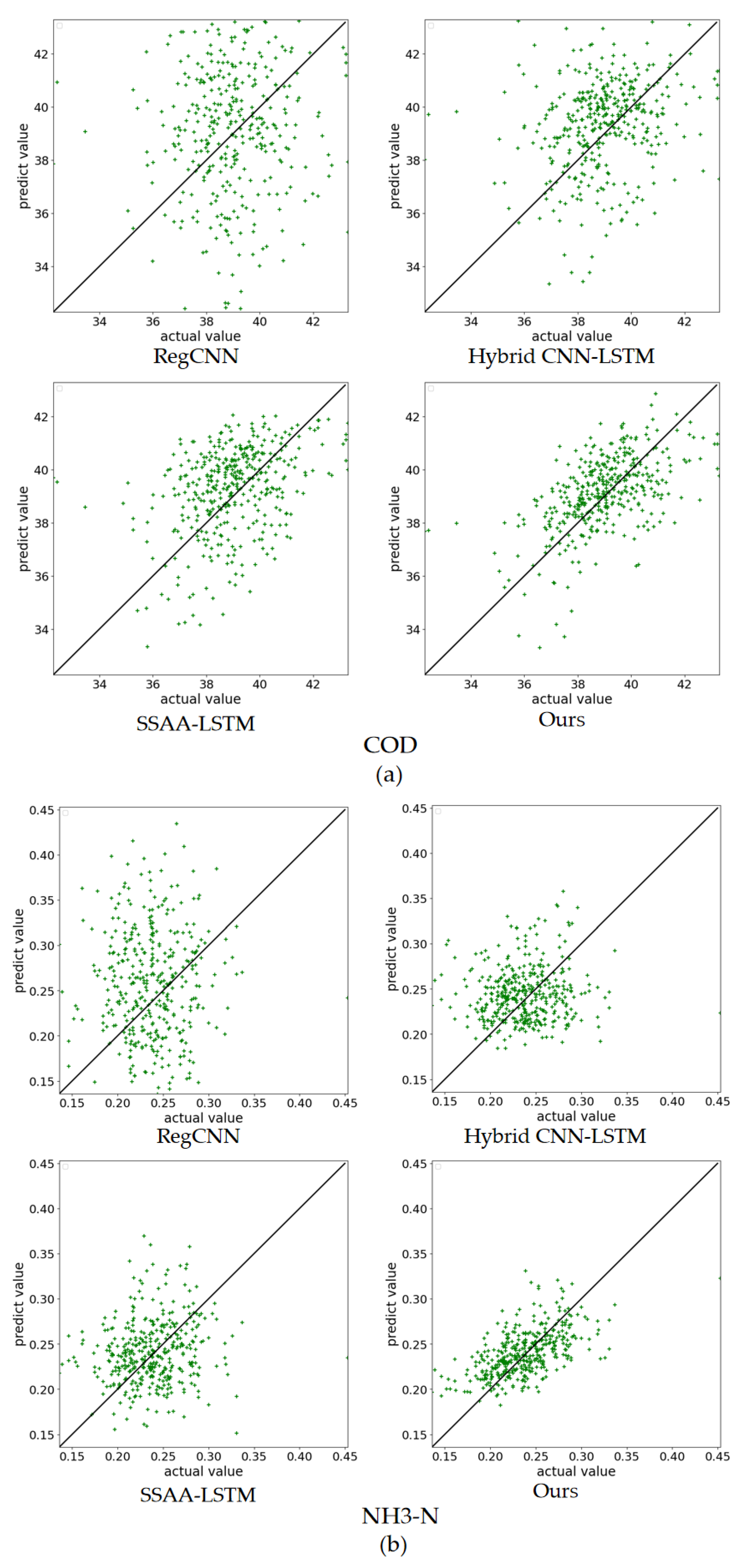
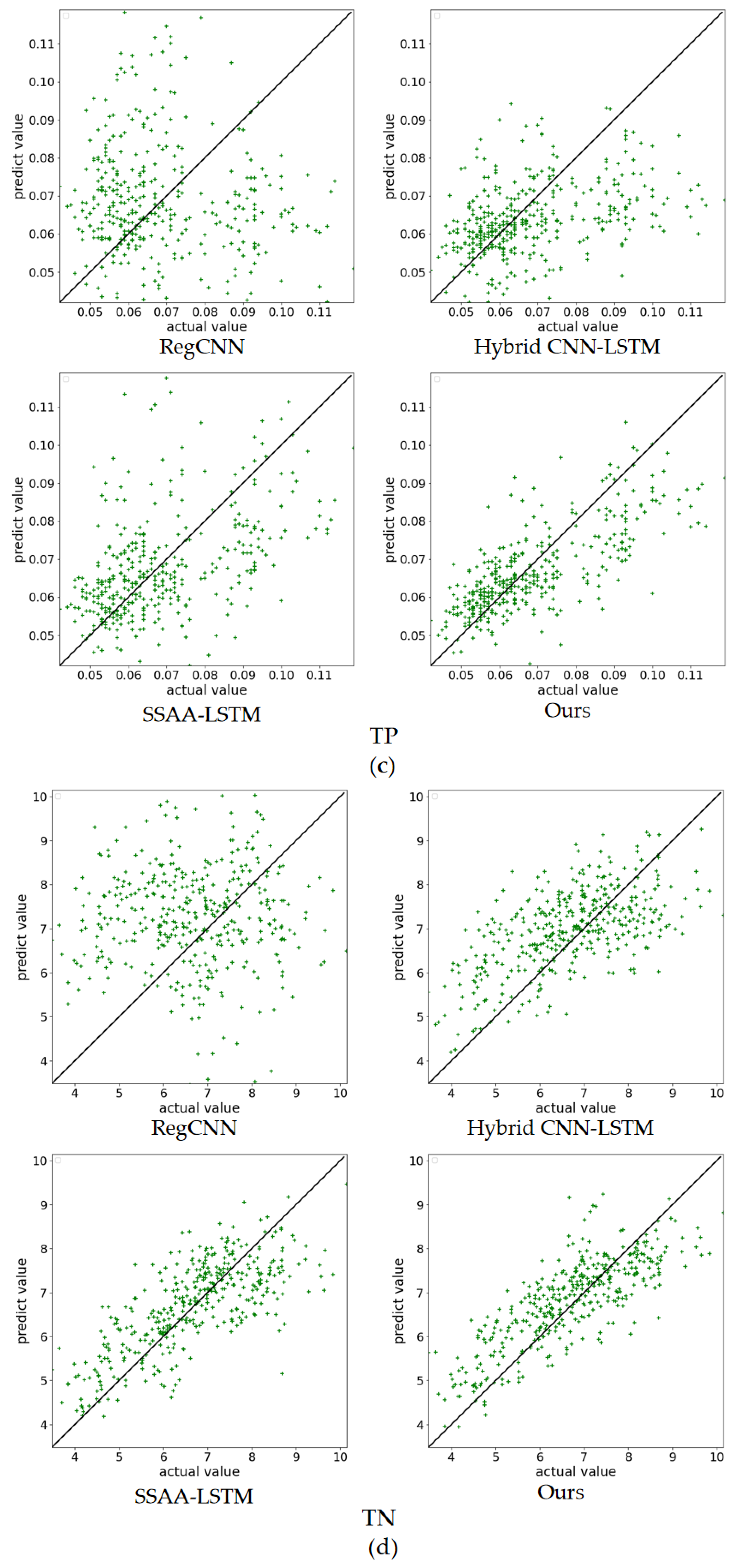
• Reg-CNN [9], based on a CNN, is used to solve multi-output regression problems and is adopted to predict effluent wastewater indicators.
• CNN-LSTM hybrid [24] is a multi-scale CNN-LSTM hybrid neural network used to make predictions in electricity load forecasting, similar to the use of the hybrid model in our method.
• SSAA-LSTM [13] is a long short-term memory network water quality prediction model based on SSA and an attention mechanism, similar to the use of an attention mechanism in our method.

4.2.2. Evaluation Indicators

• In each experiment, the three standard evaluation indicators were the Mean Square Error (MSE), Mean Absolute Percent Error (MAPE) and Limit Error Ratio (LER). MSE and MAPE were calculated as follows:

$$\mathrm{M}\mathrm{S}\mathrm{E}=\frac{1}{\mathrm{n}}\sum _{\mathrm{i}=1}^{\mathrm{n}}{({\mathrm{Y}}_{\mathrm{i}}-{\widehat{\mathrm{Y}}}_{\mathrm{i}})}^2$$

(9)

$$\mathrm{M}\mathrm{A}\mathrm{P}\mathrm{E}=\frac{1}{\mathrm{n}}\sum _{\mathrm{i}=1}^{\mathrm{n}}\frac{|{\mathrm{Y}}_{\mathrm{i}}-{\widehat{\mathrm{Y}}}_{\mathrm{i}}|}{{\mathrm{Y}}_{\mathrm{i}}}$$

(10)

where ${\mathrm{Y}}_{\mathrm{i}}$ represents the prediction value and ${\widehat{\mathrm{Y}}}_{\mathrm{i}}$ represents the actual value of wastewater quality.

LER represents the percentage of samples with more than 15% of MAPE to the total samples. The lower the LER, the higher the reliability of the predicted results.

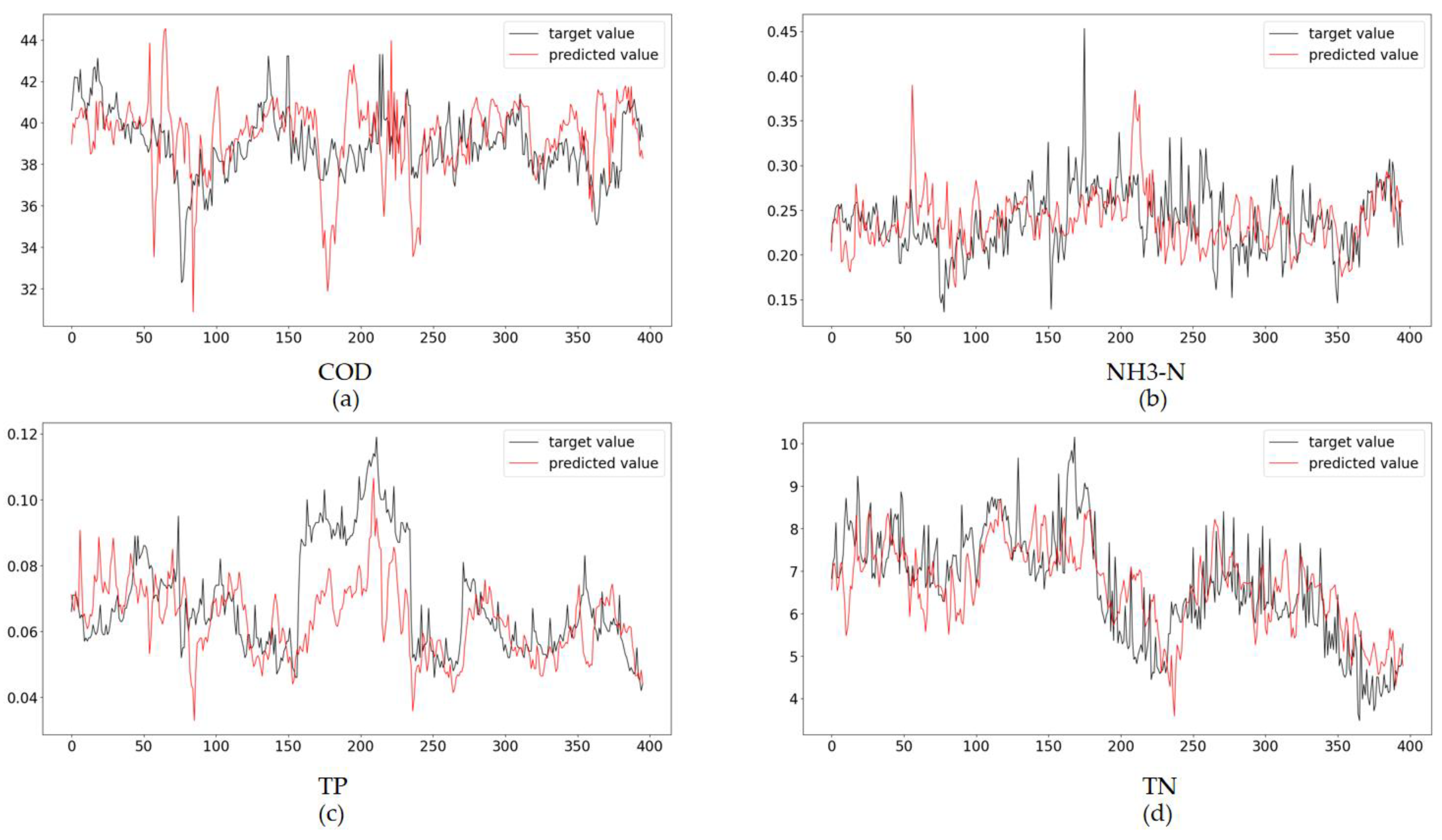
4.3. Experimental Results

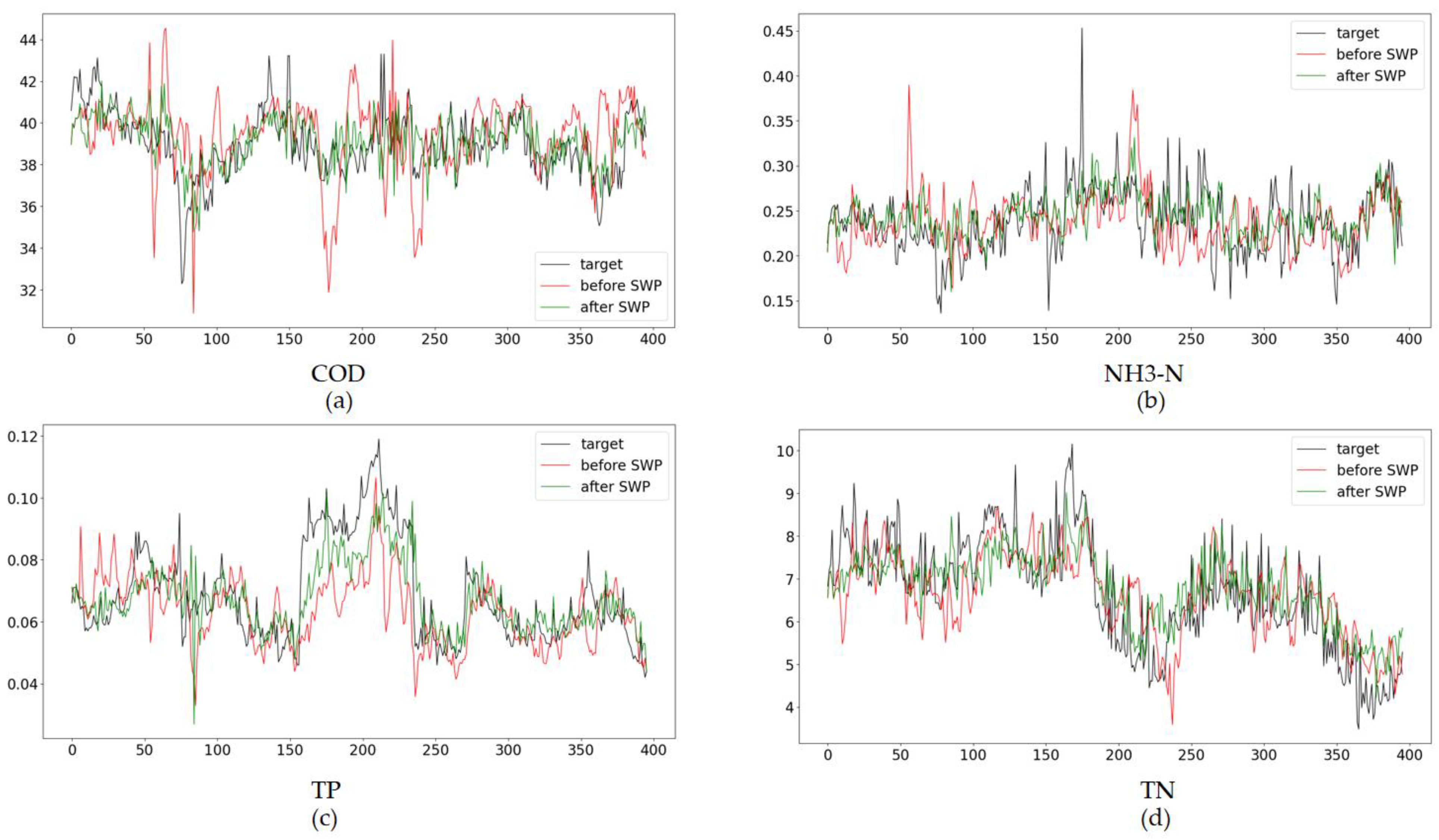
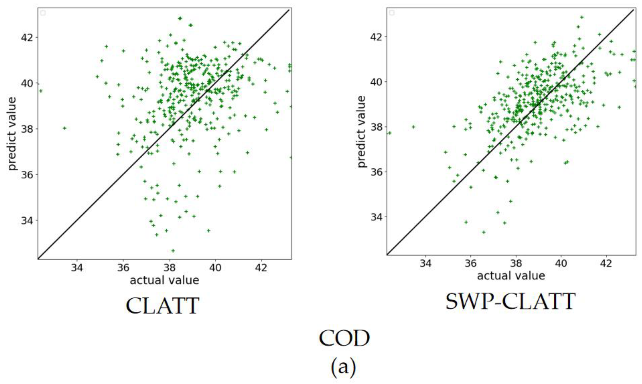
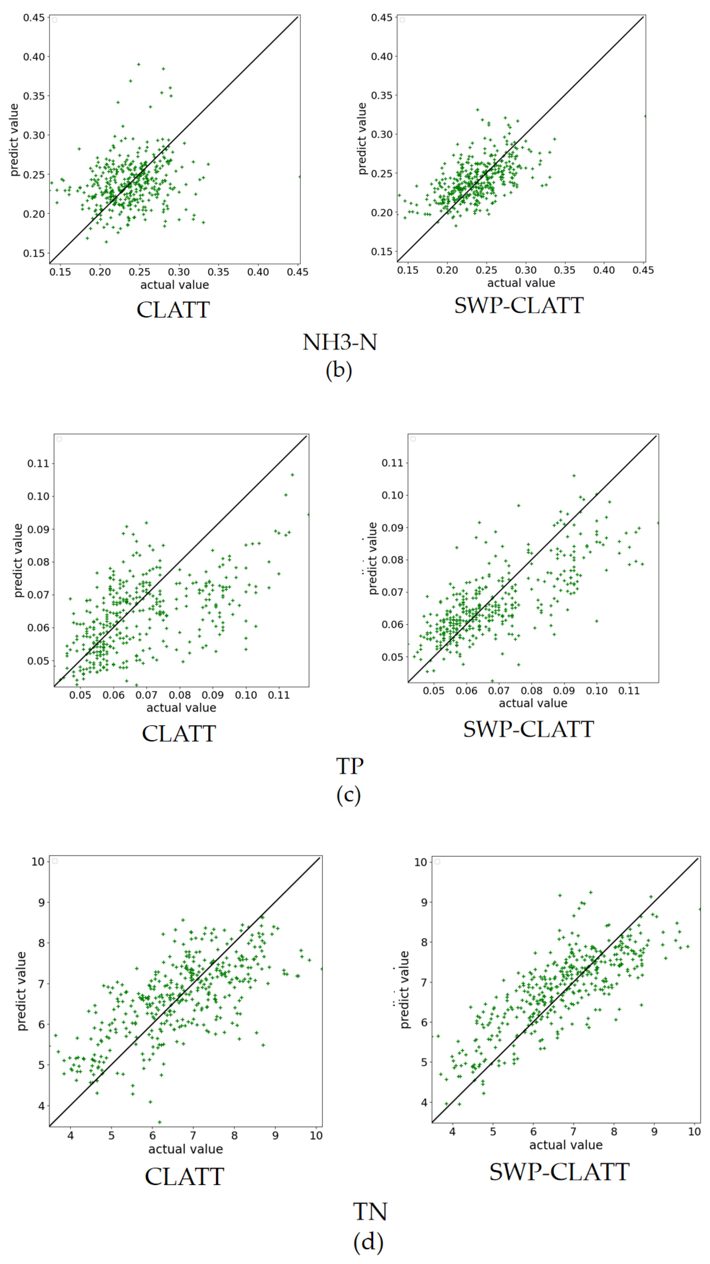
4.3.1. Comparison with Sliding Window Method

We conducted the experiment on the pre-treated dataset and selected all six influent wastewater quality indicators as the input and all four effluent wastewater quality indicators as the output of the model. According to the design, the residence time of the WWTPs was 12 h and the sampling frequency was 2 h, the interval between input and output was set as 6. After determining the input and output of the model, we put the data into the model for training. The training method adopted a fixed epoch number, and the hyperparameters of the model are shown in

Table 2. The hyperparameters of the model.

Hyperparameter	Values
3 × 3 Conv1-channel	8
3 × 3 Conv2-channel	8
1 × 1 Conv-channel	3
CNN-Dense	32
LSTM-hidden size	64
Epoch number	200
Learning rate	0.0002
Batch size	64
Optimizer	Adam

.

The 3 × 3 Conv1-channel is the number of channels in the first 3 × 3 convolution layer, the 3 × 3 Conv2-channel represents the number of channels in the second 3 × 3 convolution kernel, the 1 × 1 Conv-channel represents the number of channels in the 1 × 1 convolution kernel, and CNN-Dense represents the dimensions of the output in the Dense layer used in the CNN module. LSTM-hidden size represents the number of neurons in the LSTM layer. Epoch number, learning rate, batch size and optimizer refer to the hyperparameters of the training method.

After the training was completed, the data in the test set were fed into the model for predicting the effluent wastewater quality at once. The predicted results are shown in Figure 6.

In the figure above, the black line represents the effluent wastewater quality value, and the red line represents the effluent wastewater quality value predicted by the model. The horizontal coordinate represents the sample, and the vertical coordinate represents the concentration. It can be seen from the figure that the model can predict the general trend of effluent wastewater quality value, but for some of the large mutations, such as the middle part of the line, the predicted value differs greatly from the target value.

We calculated the MAPE value of the predicted results for 5 days, 10 days, 20 days and 30 days, as shown in Figure 7; it was found that the MAPE of all four wastewater quality indicators increases over time, which may be caused by changes in the wastewater quality conditions or the control methods of the WWTPs.

Therefore, we decided to adopt the sliding window method, similar to [25]. The idea of sliding window method is based on the following two points:

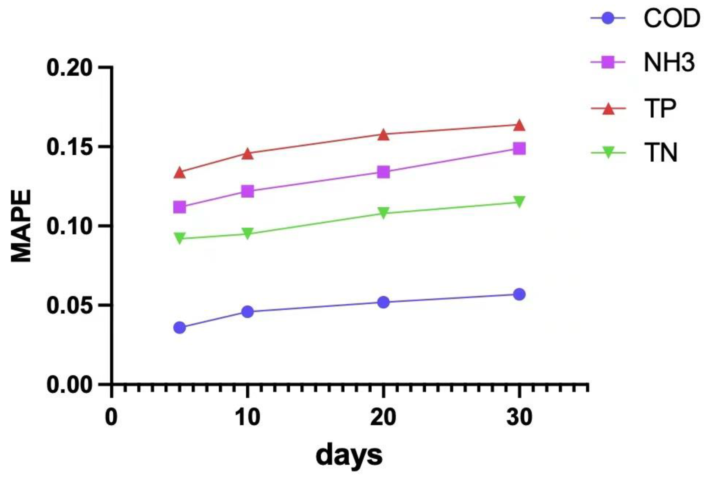
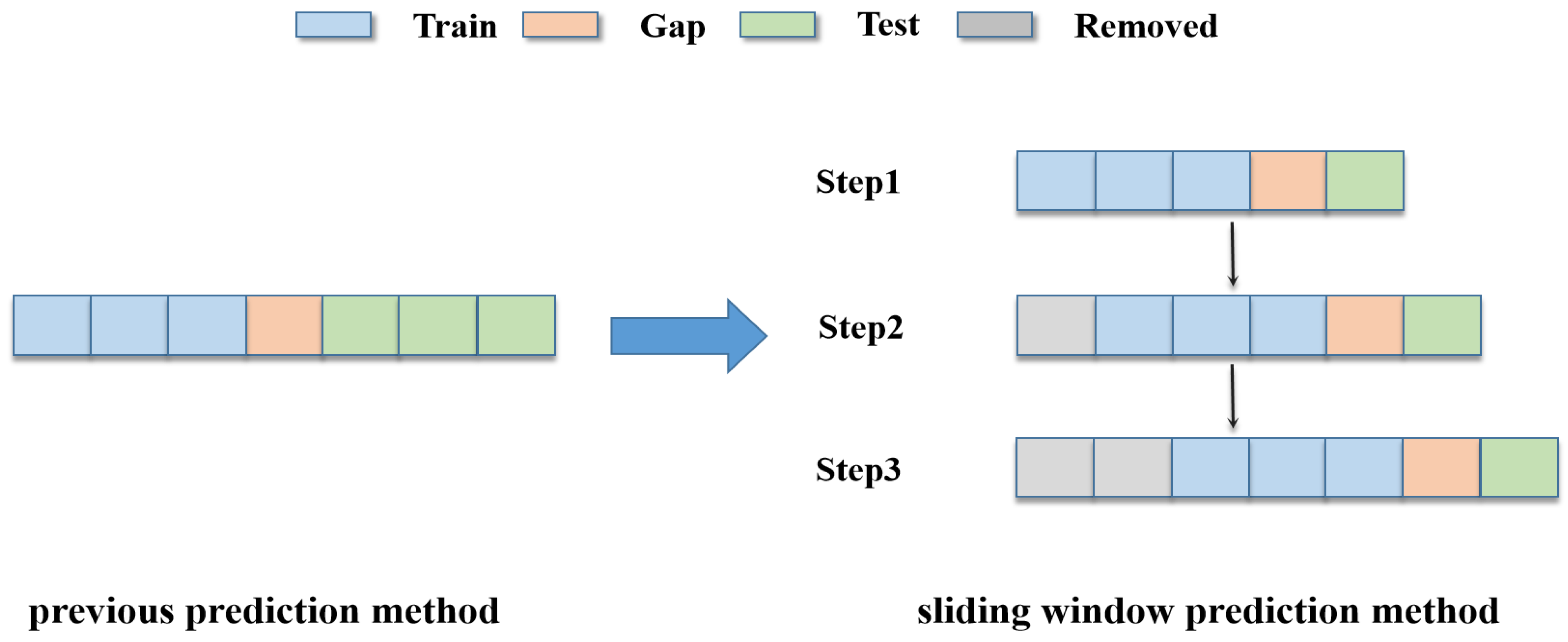
• In the daily operation of WWTPs, the effluent wastewater quality prediction model should meet the requirement of supporting dynamic updating; that is, the model will constantly update the parameters with changing time. The sliding window method simulates the dynamic updating and incremental training of the model; when a batch of new data is obtained from the WWTPs, the model is dynamically updated to improve the accuracy of the predicted results.
• Data augmentation refers to the technology of generating new training data by transforming or combining existing data. The sliding window method can also be regarded as the “data augmentation” of the datasets, which makes it easier for the model to capture the rules in the data and prevent the model from overfitting a certain section of data.

The previous prediction method predicted all the results at once, whereas the sliding window method, shown in Figure 8, breaks the process down into multiple steps. Each step only predicts the part of the test set adjacent to the training set. After completing the prediction, we slide back to proceed to the next step. Finally, the predicted results of each step are combined to obtain all of the predicted results.

The predicted results before and after using sliding window prediction (SWP) are shown in Figure 9.

In the figure, the black line represents the target values of the wastewater quality indicators, the red line represents the predicted values without using SWP, and the green line represents the predicted values with SWP. As can be seen from the image, the effect of prediction is significantly improved after using SWP. For the parts with poor prediction without using SWP, such as the middle part of the line, the prediction effect is improved after using SWP.

We also calculated the MAPE value of the predicted results for 5 days, 10 days, 20 days and 30 days, as shown in Figure 10. After using the SWP method, the prediction performance is improved in two aspects. On one hand, the accuracy of the prediction is improved, which means that for any effluent wastewater quality indicator, after using SWP, the MAPE value of the predicted result is decreased, showing that the model can achieve more accurate prediction with SWP. On the other hand, the stability of prediction is improved. In the absence of SWP, the MAPE value of the predicted results increases over time. After the sliding window is adopted, the MAPE values of the predicted results remain stable.

The SWP method can maintain stable prediction performance by constantly updating the parameters of the model, and can be used in any model of wastewater quality prediction based on neural network. In order to better compare different models, the SWP method was adopted in all subsequent experiments. Furthermore, in order to compare the predicted results of different methods more intuitively, we use the following point cloud map (PCM) to show the predicted results. The horizontal axis of the image represents the actual value, and the vertical axis represents the predicted value. The closer the point cloud on the image to the diagonal line, the more accurate the prediction results.

As can be seen from Figure 11, for the indicators COD and TP, there are a large number of discrete points with poor prediction effects on the edge of the point cloud map when SWP is not used for prediction. After SWP is used for prediction, the original discrete points on both sides of the slanted line move closer to the middle, while the point clouds converge toward the middle. For the indicators NH3 and TN, when SWP is not used, a small number of points are distributed on the edge. After SWP is used, it is difficult to find scattered points on the edge of the point cloud map.

As can be seen from

Table 3. Predicted results before and after the sliding window is used.

Method	MSE	MAPE (%)	LER (%)
CLATT	1.17	0.13	0.18
SWP-CLATT	0.92	0.08	0.11

, after using SWP, the accuracy of prediction is improved to some extent, with MSE decreasing by 0.25, MAPE decreasing by 5% and LER decreasing by 7%.

For practical engineering applications, wastewater treatment plants care more about the MAPE and LER metrics. MAPE represents the prediction accuracy of the model. The lower the MAPE value, the higher the accuracy of prediction for the whole dataset. LER represents the stability of the model under different working conditions. The lower the LER value, the fewer “mistakes” are made in the prediction results, and the stronger the stability of the model.

In summary, after SWP is used, the prediction performance of the model remains stable over time, indicating that the stability and accuracy of the prediction are improved.

4.3.2. Ablation Study

The proposed method combines a CNN, an LSTM and an attention mechanism. We conducted ablation experiments on the proposed method. The ablation experiment was divided into two parts. In the first part, we removed the CNN, the LSTM and the attention mechanism modules, respectively, as shown in

Table 4. Results of the ablation study on the parts of the model.

Model	MSE	MAPE (%)	LER (%)
CLATT	0.92	0.08	0.11
-CNN	1.30	0.17	0.18
-LSTM	1.25	0.15	0.16
-Attention	1.01	0.10	0.12

. The first row presents the results of the standard model, the second row represents the model excluding only the LSTM module, and the third row represents the model excluding only the CNN module. The last row represents the replacement of the attention mechanism in the model with a Dense layer, which is used for data dimensionality reduction and output prediction.

After removing the LSTM, the prediction performance of the model decreases significantly. Combined with the PCAF analysis of effluent wastewater quality prediction in Section 3.4, the wastewater quality at adjacent sampling times is highly correlated, and the LSTM can learn the dependence relationship in the time series, making it suitable for the prediction of wastewater quality. The function of the attention mechanism is to integrate and extract wastewater quality information at adjacent sampling times. After the removal of the attention mechanism, the prediction performance of the model decreases. After the removal of the CNN, the prediction performance decreases to a certain extent.

In another part, we evaluate the impact of several major modules of the CNN: the residual block and the BN layer. The results are shown in

Table 5. Results of the ablation study on the major modules of CNN.

Model	MSE	MAPE (%)	LER (%)
CLATT	0.92	0.08	0.11
-residual block	1.35	0.19	0.19
-BN layer	1.03	0.11	0.13

. The first row presents the results of the standard model, while the rest of the rows present the results of the variants of the standard model. In the second row, we remove the residual block in the CNN module. In the third row, the BN layer is removed.

The massive drop in evaluation indicators when the residual block is removed proves it is a pivotal step in our method. This structure ensures that original information can be transmitted further into the network and gradient explosion is avoided in training. The result also demonstrates that the BN layer is also needed to balance the contributions of each indicator in wastewater quality prediction.

4.3.3. Comparison with Other Methods

The results of SWP-CLATT on WD-1, along with the other three methods, are shown in

Table 6. Evaluation indicators of the experimental results.

Method	MSE	MAPE (%)	LER (%)
Reg-CNN [9]	4.06	0.28	0.23
CNN-LSTM hybrid [24]	1.37	0.23	0.20
SSAA-LSTM [13]	0.95	0.11	0.14
Ours	0.92	0.08	0.11

. The number of parameters and the training times of each sliding window step of the different methods are shown in

Table 7. Parameters and training times of the different methods.

Method	Parameters	Training Time
Reg-CNN [9]	52,289	0.6
CNN-LSTM hybrid [24]	77,617	2.66
SSAA-LSTM [13]	69,636	2.3
Ours	54,955	2.17

. All methods use the same data preprocessing method and SWP training method as us.

As can be seen from Table 5, compared with the Reg-CNN, SSAA-LSTM, CNN-LSTM hybrid and our method all contain an LSTM module, and decrease by more than 2.69 in MSE, 5% in MAPE, and 3% in LER. There are two reasons for the poor prediction performance of Reg-CNN. On one hand, wastewater quality contains time series information, which is difficult to extract using the CNN network. On the other hand, the wastewater treatment process contains complex biochemical reactions and requires highly nonlinear models for simulation. Reg-CNN is a single CNN model whose modeling ability is insufficient to simulate wastewater treatment.

In the model using the LSTM, both SSAA-LSTM and our method adopt the attention mechanism, which decreases MSE, MAPE and LER by over 0.42, 12% and 6% compared to the CNN-LSTM hybrid. This is because the attention mechanism can enhance the screening and concentration of wastewater quality information at adjacent sampling times so as to focus on important features. Compared with SSAA-LSTM, our method decreases MSE, MAPE and LER by 0.03, 3% and 3%, which is because the hybrid neural network can improve the nonlinear modeling ability of the model and reduce the overfitting phenomenon. Two-dimensional convolution is adopted to extract the feature information in the time dimension and the feature dimension. Wastewater quality at adjacent sampling times is highly correlated, and the feature information can be effectively extracted and encoded by the 2D convolutional neural network.

In comparison with the model parameters and training time, Reg-CNN achieves the best performance, which is because CNN supports parallel computation. The next state of the LSTM depends on the previous state, which cannot support parallel computation. Therefore, the training time of the model containing the LSTM is longer. Among all the models containing an LSTM, our method achieves the fastest training time and the lowest number of parameters due to the two Dense layers used in the CNN to reduce the number of parameters.

The experimental results with images are displayed in Figure 12.

The horizontal axis of the picture represents the actual values, and the vertical axis represents the predicted values. The closer the distance between dots and slashes on the image, the more stable the prediction. As can be seen from the image, compared with the CNN method, the LSTM method has more advantages. Compared with the other methods, the point cloud map drawn using our method is denser and the predicted values are distributed near the actual values. In summary, our method achieves the optimal prediction performance and maintains the best stability.

5. Conclusions

In this article, we present CLATT, which uses the CNN-LSTM-Attention structure as its backbone. Seven-month wastewater quality data collected from WWTP were used to validate the effectiveness of the proposed method. We conducted numerous comparative experiments and an ablation study. In order to eliminate the decreasing trend of prediction performance over time, a sliding window method is proposed to improve the prediction accuracy and stability of the model. In addition, an ablation study was conducted on the main structure of the model to verify its rationality. Finally, compared with other methods, the proposed method achieved optimal performance on different evaluation indicators, and realized the most efficient prediction among all the methods based on the LSTM. Future work will focus on the following:

• Improving the generalization performance of the model. The proposed method in this paper is mainly used for the data of municipal WWTPs. However, in practical application, the wastewater quality condition of WWTPs varies with different water sources. For example, the COD of chemical wastewater is higher than that of municipal wastewater. Different water quality conditions will affect the prediction performance of the method. The method proposed in this paper may not be suitable for use in WWTPs from other water sources. Future work could consider building more general models to adapt to the data characteristics of different WWTPs and improve the generalization performance of the method.
• Adding the means of operation in WWTPs to the input of the model. The sampling information of WWTPs only includes the indicators of influent and effluent wastewater quality; it does not include the means of operation, such as the dosage of commonly used chemicals in WWTPs and the aeration capacity of the blower, which are also important factors affecting the quality of effluent wastewater. The proposed method in this paper is only based on the use of influent wastewater quality to predict effluent wastewater quality. In the future, the operation methods of WWTPs could be added to realize the prediction of effluent wastewater quality under the condition of complete data collection.

References

1. Samuelssona, P.; Halvarsson, B.; Carlsson, B. Cost-efficient operation of a denitrifying activated sludge process. Water Res. 2007, 41, 2325–2332. [Google Scholar] [CrossRef] [PubMed]
2. Coelho, M.A.Z.; Russo, C.; Araújo, O.Q.F. Optimization of a sequencing batch reactor for biological nitrogen removal. Water Res. 2000, 34, 2809–2817. [Google Scholar] [CrossRef]
3. Gujer, W.; Henze, M.; Mino, T.; Van Loosdrecht, M. Activated sludge model no. 3. Water Sci. Technol. 1999, 39, 183–193. [Google Scholar] [CrossRef]
4. Grau, P.; Beltrán, S.; De Gracia, M.; Ayesa, E. New mathematical procedure for the automatic estimation of influent characteristics in WWTPs. Water Sci. Technol. 2007, 56, 95–106. [Google Scholar] [CrossRef] [PubMed]
5. Kim, Y.; Kim, M.; Yoo, C. A new statistical framework for parameter subset selection and optimal parameter estimation in the activated sludge model. J. Hazard. Mater. 2010, 183, 441–447. [Google Scholar] [CrossRef] [PubMed]
6. Pakrou, S.; Mehrdadi, N.; Baghvand, A. Artifificial neural networks modeling for predicting treatment effificiency and considering effects of input parameters in prediction accuracy: A case study in tabriz treatment plant. Indian J. Fundam. Appl. Life Sci. 2014, 4, 2231–6345. [Google Scholar]
7. Nourani, V.; Elkiran, G.; Abba, S. Wastewater treatment plant performance analysis using artifificial intelligence—An ensemble approach. Water Sci. Technol. 2018, 78, 2064–2076. [Google Scholar] [CrossRef] [PubMed]
8. Wang, D.; Thunéll, S.; Lindberg, U.; Jiang, L.; Trygg, J.; Tysklind, M.; Souihi, N. A machine learning framework to improve effluent quality control in wastewater treatment plants. Sci. Total Environ. 2021, 784, 147138. [Google Scholar] [CrossRef] [PubMed]
9. Zhang, L.; Ma, X.; Shi, P.; Bi, S.; Wang, C. RegCNN: A Deep Multi-output Regression Method for Wastewater Treatment. In Proceedings of the IEEE 31st International Conference on Tools with Artificial Intelligence (ICTAI), Portland, OR, USA, 4–6 November 2019; pp. 816–823. [Google Scholar]
10. Li, X.; Yi, X.; Liu, Z.; Liu, H.; Chen, T.; Niu, G.; Yan, B.; Chen, C.; Huang, M.; Ying, G. Application of novel hybrid deep leaning model for cleaner production in a paper industrial wastewater treatment system. J. Clean. Prod. 2021, 294, 126343. [Google Scholar] [CrossRef]
11. Jafar, R.; Awad, A.; Jafar, K.; Shahrour, I. Predicting Effluent Quality in Full-Scale Wastewater Treatment Plants Using Shallow and Deep Artificial Neural Networks. Sustainability 2022, 14, 15598. [Google Scholar] [CrossRef]
12. Wan, X.; Li, X.; Wang, Z.; Yi, X.; Zhao, Y.; He, X.; Wu, R.; Huang, M. Water quality prediction model using Gaussian process regression based on deep learning for carbon neutrality in papermaking wastewater treatment system. Environ. Res. 2022, 211, 112942. [Google Scholar] [CrossRef] [PubMed]
13. Wang, X.F.; Wei, S.N.; Xu, L.X.; Pan, J.; Wu, Z.Z.; Kwong, T.C.; Tang, Y.Y. LSTM Wastewater Quality Prediction Based on Attention Mechanism. In Proceedings of the International Conference on Wavelet Analysis and Pattern Recognition (ICWAPR), Adelaide, Australia, 4–5 December 2021; pp. 1–6. [Google Scholar]
14. Srinivasan, S.; Ravi, V.; Sowmya, V.; Krichen, M.; Noureddine, D.B.; Anivilla, S.; Soman, K.P. Deep Convolutional Neural Network Based Image Spam Classification. In Proceedings of the Conference on Data Science and Machine Learning Applications (CDMA), Riyadh, Saudi Arabia, 4–5 March 2020; pp. 112–117. [Google Scholar]
15. He, K.; Zhang, X.; Ren, S.; Sun, J. Deep Residual Learning for Image Recognition. In Proceedings of the IEEE Conference on Computer Vision and Pattern Recognition (CVPR), Las Vegas, NV, USA, 27–30 June 2016; pp. 770–778. [Google Scholar]
16. Hochreiter, S.; Schmidhuber, J. Long Short-Term Memory. Neural Comput. 1997, 9, 1735–1780. [Google Scholar] [CrossRef] [PubMed]
17. Tzirakis, P.; Zhang, J.; Schuller, B.W. End-to-End Speech Emotion Recognition Using Deep Neural Networks. In Proceedings of the IEEE International Conference on Acoustics, Speech and Signal Processing (ICASSP), Calgary, AB, Canada, 15–20 April 2018; pp. 5089–5093. [Google Scholar]
18. Breuel, T.M. High-Performance Text Recognition Using a Hybrid Convolutional-LSTM Implementation. In Proceedings of the IAPR International Conference on Document Analysis and Recognition (ICDAR), Kyoto, Japan, 9–15 November 2017; pp. 11–16. [Google Scholar]
19. Pielka, M.; Sifa, R.; Hillebrand, L.P.; Biesner, D.; Ramamurthy, R.; Ladi, A.; Bauckhage, C. Tackling Contradiction Detection in German Using Machine Translation and End-to-End Recurrent Neural Networks. In Proceedings of the International Conference on Pattern Recognition (ICPR), Milan, Italy, 10–15 January 2021; pp. 6696–6701. [Google Scholar]
20. Zhu, J.; Zurcher, J.; Rao, M.; Meng, M.Q. An on-line wastewater quality prediction system based on a time-delay neural network. Eng. Appl. Artif. Intell. 1998, 11, 747–758. [Google Scholar] [CrossRef]
21. Memarzadeh, G.; Keynia, F. Short-term electricity load and price forecasting by a new optimal LSTM-NN based prediction algorithm. Electr. Power Syst. Res. 2021, 192, 106995. [Google Scholar] [CrossRef]
22. Mnih, V.; Heess, N.; Graves, A.; Kavukcuoglu, K. Recurrent models of visual attention. In Proceedings of the 27th International Conference on Neural Information Processing Systems—Volume 2 (NIPS’14); 2014; pp. 2204–2212. [Google Scholar]
23. Tabelini, L.; Berriel, R.; Paixao, T.M.; Badue, C.; De Souza, A.F.; Oliveira-Santos, T. Keep your Eyes on the Lane: Real-time Attention-guided Lane Detection. In Proceedings of the IEEE/CVF Conference on Computer Vision and Pattern Recognition (CVPR), Nashville, TN, USA, 20–25 June 2021; pp. 294–302. [Google Scholar]
24. Guo, X.; Zhao, Q.; Zheng, D.; Ning, Y.; Gao, Y. A short-term load forecasting model of multi-scale CNN-LSTM hybrid neural network considering the real-time electricity price. Energy Rep. 2020, 6, 1046–1053. [Google Scholar] [CrossRef]
25. Huang, S.; Shen, J.; Lv, Q.; Zhou, Q.; Yong, B. A Novel NODE Approach Combined with LSTM for Short-Term Electricity Load Forecasting. Future Internet 2023, 15, 22. [Google Scholar] [CrossRef]
Figure 1. Overview of the proposed method called CLATT. It receives a sequence of wastewater quality indicators taken from real-world wastewater treatment plants. The encoder is formed of a CNN module with a residual block. A standard LSTM module is regarded as a decoder. The attention mechanism module is used to integrate information and make predictions.
Applsci 13 07011 g001
Figure 2. The input and output of the model.
Applsci 13 07011 g002
Figure 3. CNN-LSTM structure.
Applsci 13 07011 g003
Figure 4. (a) PACF of effluent COD with 10 lags; (b) PACF of effluent NH3-N with 10 lags; (c) PACF of effluent TP with 10 lags; (d) PACF of effluent TN with 10 lags.
Applsci 13 07011 g004
Figure 5. Attention mechanism used in CLATT.
Applsci 13 07011 g005
Figure 6. (a) Target and predicted values of COD; (b) target and predicted values of NH3-N; (c) target and predicted values of TP; (d) target and predicted values of TN.
Applsci 13 07011 g006
Figure 7. The trend of the results.
Applsci 13 07011 g007
Figure 8. Sliding window method.
Applsci 13 07011 g008
Figure 9. (a) The target and predicted values of COD before and after using SWP; (b) the target and predicted values of NH3-N before and after using SWP; (c) the target and predicted values of TP before and after using SWP; (d) the target and predicted value of TN before and after using SWP.
Applsci 13 07011 g009
Figure 10. The trend of MAPE before and after using SWP in COD.
Applsci 13 07011 g010
Figure 11. PCMs showing (a) the target and predicted values of COD before and after using SWP; (b) the target and predicted values of NH3-N before and after using SWP; (c) the target and predicted values of TP before and after using SWP; (d) the target and predicted values of TN before and after using SWP.
Applsci 13 07011 g011aApplsci 13 07011 g011b
Figure 12. PCMs of (a) the target and predicted values of COD with four methods; (b) the target and predicted values of NH3-N with four methods; (c) the target and predicted values of TP with four methods; (d) the target and predicted values of TN with four methods.
Applsci 13 07011 g012aApplsci 13 07011 g012b