The Improvement of the Honey Badger Algorithm and Its Application in the Location Problem of Logistics Centers

Featured Application

This paper studies the joint optimization of the threshold setting of large parcels, the location selection of multi-functional transit centers, and the allocation of terminal demand points under the implementation of multi-product (parcel) distribution by urban logistics enterprises, which is a new extension of the urban logistics site selection-path problem. Through this article, constructive suggestions are put forward for the future development of large-scale businesses in the logistics field, and other logistics companies can make a comprehensive assessment according to their own needs and conditions.

Abstract

Aiming at the problems of low resource utilization and high distribution cost of urban logistics enterprises, this paper introduces the threshold setting of large parcels, comprehensively considers the processing links of large parcels and standard parcels in loading, unloading, sorting, and other processing links, and constructs a logistics planning model with the type of multi-functional transit center as the variable and the total cost of the logistics system as the goal. Aiming at the shortcomings of the honey badger algorithm, three optimization strategies are used to improve the logistics model, and the effectiveness of the improved algorithm is verified by comparing with the CPLEX operation results. Based on the operation data of SF Jinzhou, this paper obtains the optimization results of large parcel threshold, multi-function transit center location layout, and terminal demand point allocation. From the results, the introduction of the threshold setting for large parcels has played a significant role in the joint optimization of multi-functional center location selection and terminal demand point allocation under multi-parcel distribution and provides theoretical data support for the existing urban logistics location problem.

1. Introduction

1.1. Current Situation of Urban Logistics Enterprises

With the gradual improvement of modern logistics network, there are more and more categories of logistics distribution, from letters, daily necessities, and electronic products to large commodities such as home appliances and homes. The shape and weight of logistics packages change, and urban logistics enterprises mainly divide them into bulky parcels and standard parcels. Oversized parcels, also known as weighed parcels, refer to parcels whose weight or volume exceeds a certain threshold. Typical oversized parcels include e-commerce bulky items such as home appliances and home furnishing for end consumers, replenishment bulky items for various offline physical stores, and moving bulky items for relocated groups. At present, there is no uniform standard for the threshold of large parcels in the industry, and there are differences between different companies. For example, express companies such as Deppon and ANE have lower thresholds, such as the Deppon threshold of 3 kg and the ANE logistics threshold of 5 kg. However, express delivery companies such as ZTO, SF Express, and YTO have higher thresholds, such as ZTO Express with a threshold of 10 kg, SF Express with a heavy parcel threshold of 20 kg, and YTO E-commerce with a threshold of 30 kg. Bulky parcel threshold settings affect urban logistics site selection and route planning.

A typical urban logistics network includes urban distribution centers, urban transit centers, and end-of-line demand points close to customers. Generally speaking, for standard packages, the specifications and standards include small weight and volume, low wear rate, and low requirements for sorting facilities, handling tools and logistics sites. However, the volume or weight of large parcels is large and the packaging shape is irregular, the parcel value is high, it is easy to wear, and the requirements for sorting facilities, handling tools, and logistics sites are high. As a result, there are significant differences between bulky parcel transit centers and standard express parcel transit centers in terms of capacity configuration, sorting facilities, and handling loading and unloading tools. The location of bulky and standard parcel transit centers also affects urban logistics site selection and route planning.

At present, logistics enterprises mainly adopt the independent distribution mode of sub-network for standard parcels and bulky parcels, with low resource utilization and high distribution costs, and multi-type parcel collaborative distribution is an effective strategy for integrated logistics enterprises to solve urban distribution. Collaborative distribution refers to the centralized dispatch of logistics resources such as logistics facilities, transit centers, terminal outlets, distribution vehicles, and front-line employees to meet the collection and delivery needs of various types of logistics parcels. According to the demand characteristics of various packages, joint optimization of large parcel threshold setting, transit center location selection, and terminal demand point allocation (transit center coverage) is the key to implementing coordinated distribution.

1.2. Research Status and Significance at Home and Abroad

In view of the problem of logistics center site selection, domestic and foreign research is mainly divided into two aspects; one is to solve this problem through mathematical and physical methods [1,2,3,4] and methods such as the analytic hierarchy method, center of gravity method, and dynamic programming method are proposed, which have made breakthrough progress in solving the problem of logistics distribution center site selection, such as [1] using the optimal worst criterion decision-making method to optimize the location of logistics center; ref. [2] combines the Gauss–Kruger projection inversion algorithm with the center of gravity method to optimize the location of distribution centers between four cities in Zhejiang Province; in [3], the K-Means algorithm and center of gravity method are used to select the location of logistics centers; ref. [4] uses analytic hierarchy to solve the problem of logistics center site selection. This type of method adopts mathematical or physical methods, although the algorithm structure is relatively simple, but the algorithm steps are more, the accuracy of the results is slightly poor, there is a certain error, and it is less involved in the current relevant research in this field. Another aspect is to use various intelligent optimization algorithms to solve the problem of logistics site selection-path optimization. Among them, most scholars use heuristic algorithms or meta-heuristics or hybrid heuristics [5,6,7,8,9,10,11,12,13,14,15], such as cuckoo search algorithm, gray wolf optimization algorithm, ant colony algorithm, genetic algorithm, simulated annealing algorithm, differential evolution strategy algorithm, etc., which are suitable for medium-scale and large-scale problems. The authors of [5] use the longhorn beetle search-rainfall algorithm for the site selection of logistics center; in [6], the differential evolution strategy is used to improve the cuckoo search algorithm to improve the accuracy of logistics center site selection. The authors of [7] use gray wolf optimization algorithm to optimize this problem; ref. [8] improved the whale optimization algorithm to study this problem; ref. [9] uses the improved ant colony algorithm to optimize logistics and distribution routes. The authors of [10] use the optimization of logistics distribution route using a genetic algorithm; simulated annealing algorithm and simulated annealing technology are proposed in [11]; ref. [12] uses particle swarm optimization for logistics center site selection; ref. [13] proposes an adaptive particle swarm optimization algorithm with nonlinear inertia weights and time-varying acceleration coefficients to study the distribution problem to control the balance of global search and local search for the distribution center position problem; ref. [14] introduces ant colony optimization algorithm for clustering and ant colony optimization algorithm for finding the shortest path and assigns customers and distribution centers to the model, respectively; ref. [15] adopts the improved bat algorithm, reasonably sets the parameters and selection operators in the algorithm, and solves the model to improve the prediction accuracy of logistics center site selection. Although the use of intelligent algorithms can effectively improve the speed of solving the site selection problem, the problem is that intelligent algorithms are prone to fall into convergence stagnation caused by local optimization in the optimization process, which is the problem faced by intelligent algorithms in the research of this problem. In addition, some researchers have studied the site selection problem through machine learning methods [16,17,18], but this type of method to solve the problem requires a large amount of data to train the model, resulting in too high complexity, and the time required far exceeds the use of intelligent algorithms, the learning time is too long, and even the purpose of learning cannot be achieved.

Among them, the swarm intelligence algorithm is inspired by the movement of biological populations in nature, predation, and other behaviors, and a class of algorithms has been proposed; at present, a large number of swarm intelligence algorithms have been proposed at home and abroad [19,20,21,22,23,24,25,26,27]. These algorithms are widely used in solving practical engineering optimization problems and have objective effects. The logistics site path optimization problem is a typical NP-hard probability problem. In recent years, most of the research in this field has used swarm intelligence algorithms [28] to solve such nonlinear optimization problems. In the face of such problems, swarm intelligence algorithms often have very considerable optimization effects, so it is proposed to use swarm intelligence algorithms to optimize the location problem of logistics centers.

Similarly, I draw on research conducted by academics in the field of logistics center site selection—for example, the problem of warehouse location in supply chain design studied in [29] and delivery issues in distribution systems for urban agglomerations considered in [30].

In summary, with the deepening of the relevant research on group intelligent algorithms at home and abroad in recent years, in the direction of logistics center site selection, the use of an intelligent algorithm with high accuracy and relatively simple structure is a good idea, and a method that can accurately and simply solve the problem of logistics center location is developed, which is intended to reduce the additional cost caused by traditional methods, improve the operational efficiency of logistics centers, and then improve the efficiency of corresponding industries. Intelligent algorithm is an excellent method of optimal value optimization, as it can conduct a more comprehensive search of the map and select the optimal location of the logistics center; in the face of a series of shortcomings brought by the traditional method, the logistics site selection based on the intelligent algorithm can effectively solve the timeliness and cost problems in the location problem of the logistics center. Aiming at the problem that traditional heuristic algorithms are prone to fall into local optimization in solving the problem of location selection of logistics distribution centers, resulting in reducing the efficiency of logistics system, an improved optimization algorithm is proposed, which can effectively improve the operating rate of logistics systems.

2. Research Status and Significance at Home and Abroad

Based on the urban distribution practice of bulky parcels and standard parcels, this paper constructs a joint optimization model for the threshold setting of oversized parcels and standard parcels, the location selection of multi-function transit centers, and the allocation of terminal demand points under the coordinated distribution of bulky parcels and standard parcels, considering the capacity constraints of transit centers and the different requirements of parcels (weight or volume), processing costs, and facility configurations.

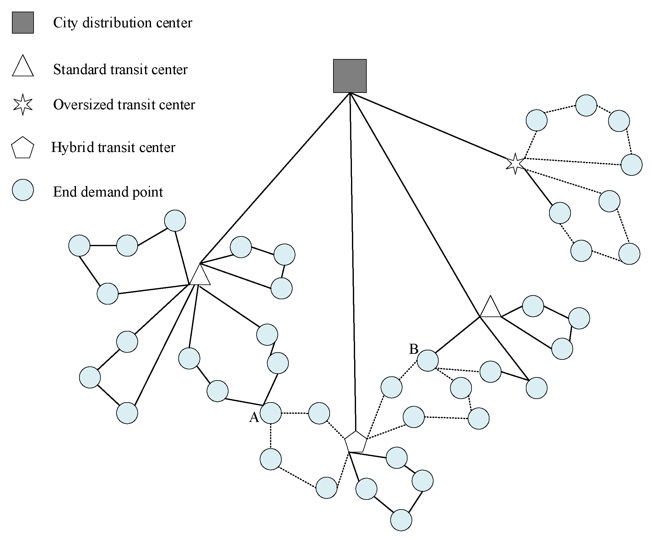
2.1. Describe the Problem

A typical urban logistics network includes urban distribution centers, urban transit centers, and end-of-line demand points close to customers. The city distribution center is responsible for the inflow and outflow of goods (or parcels) in the city. The transit center connects the distribution center and the terminal demand point and is responsible for transit processing. The terminal demand point is generally located in the community, school, business district, and other locations, responsible for the delivery and collection of parcels in the area.

When standard parcels and oversized parcels are delivered together, according to the functional differences, transit centers can be divided into three categories: oversized transit centers, standard transit centers and hybrid transit centers. In practice, most of the point-to-point direct distribution mode is adopted between the distribution center and the transit center, and the circular distribution mode is adopted between the transit center and the terminal demand point. From the transit center to the end demand point, standard parcels and bulky parcels are independently distributed and collected, the solid line between the terminal demand points in Figure 1 represents the standard parcel travel route, and the dotted line between the end demand points represents the oversized parcel travel route. When the terminal demand point has both standard parcel and bulky parcel delivery or collection demand, it needs to be accessed twice separately, as shown in point A and point B in Figure 1. Urban logistics enterprises face the following decision-making problems when implementing multi-type parcel collaborative distribution:

• Threshold setting for bulky parcels and standard parcels;
• The number and location of three types of transit centers: large-size, standard, and mixed;
• The coverage of transit centers of different functional types, that is, the allocation of terminal demand points.

2.2. Model Building

The above joint optimization problem is an extension of the capacity-limited two-level site-path problem, which is defined in a fully weighted directed network $G=\left(V,A\right)$, where $V=\left(V_0,V_1\right)$ represents the collection of logistics nodes, $V_0$ represents the city distribution center, $V_1=\left(P,Q\right)$, M and N represent the set of candidate points of transit center and the set of terminal demand points, respectively. The arc set A is defined as $A=\left(A_1\cup A_2\right)$, $A_1=\left\{\left(0,p\right):0\in V_0,p\in P\right\}$, $A_2=\left\{\left(i,j\right):i,j\in V_1,i\ne j,\left(i\cup j\right)\cap Q\ne \varnothing \right\}$. Model $v_1$ is adopted from the city distribution center to the transit center, and the standard parcel and the large parcel at the end-of-service demand point of the transit center are selected as the model $v_2$ and $v_3$, respectively.

To establish the joint optimization model, set the following parameters and decision variables:

• Model parameters:

$V_0$: City Distribution Center;

P: Collection of candidate points of transit center;

$Q$: Set of end demand points;

M: Collection of package types;

f_s: Fixed costs of standard transit centers, such as site costs, sorting, loading and unloading, and handling supporting facilities;

$f_L$: Fixed costs of bulky transit centers, such as site costs, sorting, loading and unloading, and handling supporting facility costs;

$f_{MIX}$: Fixed costs of hybrid transit centers, such as site costs, sorting, loading and unloading, and handling supporting facilities;

$N_p$: The maximum capacity of the candidate point $p$ of the transit center, expressed by the number of packages, related to the size of the package, and changes accordingly with different thresholds, $p\in P$;

$d_{op}$: Distance from the city distribution center to the alternative transit center $p$, $p\in P$;

$c_{v1}$, $c_{v2}$, $c_{v3}$: Indicates the unit transportation cost of models $v_1$, $v_2$ and $v_3$ respectively;

cap_v1, cap_v2, cap_v3: The maximum loading capacity of models $v_1$, $v_2$, and $v_3$ are, respectively, expressed by the number of packages; for the same model, the number of packages under different large parcel threshold selections is different;

$w_m$: The weight of the m type parcel is converted into a joint measurement of weight and volume for light dumping with a large volume;

$C_s$: The unit handling cost of standard parcels, including handling and unloading costs and sorting costs in transit centers, loading and unloading costs at end demand points, etc., mainly depends on the average weight of standard parcels and is affected by parcel threshold settings;

$C_l$: The unit processing cost of bulky parcels, including handling, loading and unloading costs and sorting costs in transit centers, loading and unloading costs at end demand points, etc., mainly depends on the average weight of bulky parcels and is affected by parcel threshold settings;

$D_{i,m}^{Pick}$, $D_{i,m}^{Del}$: indicates the number of packages collected and delivered by $m$ type parcels at the end demand point $i$, respectively, $i\in Q$, $m\in M$;

$D_{j,m}^{Pick}$, $D_{j,m}^{Del}$: indicates the number of packages collected and delivered by $m$ type parcels at the end demand point $j$, respectively, $j\in Q$, $m\in M$;

$D_{Sta}^{Pick}$, $D_{Sta}^{Del}$, $D_{Ove}^{Pick}$, $D_{Ove}^{Del}$: respectively, the total quantity of standard parcel collection and distribution at the end demand point, the total quantity of oversized parcel collection and delivery, and the threshold selection of different oversized parcels is also different;

$l_{ij}^{v2}$: the standard parcel volume loaded by vehicle v2 from node i to node j, including collection and delivery volume, $i,j\in V_1$, $i\ne j$, $\left(i\cup j\right)\cap Q\ne \varnothing$;

$l_{ij}^{v3}$: the volume of bulky parcels loaded by vehicle v3 from node i to node j, including collection and delivery volume, $i,j\in V_1$, $i\ne j$, $\left(i\cup j\right)\cap Q\ne \varnothing$;

$L_p^{s,Pick}$: indicates the total collection volume of standard parcels processed by the transit center $p$, $p\in P$;

$L_p^{s,Del}$: indicates the total delivery volume of standard parcels processed by the transit center p, p ∈ P;

$L_p^{l,Pick}$: indicates the total collection volume of bulky parcels processed by the transit center $p$, $p\in P$;

$L_p^{l,Del}$: indicates the total delivery volume of bulky parcels processed by the transit center $p$, $p\in P$;

$t_i^{v2}$: indicates the total time used when vehicle $v_2$ departs from the transit center and arrives at node $i$;

$t_i^{v3}$: indicates the total time used when vehicle $v_3$ departs from the transit center and arrives at node $i$;

$t_{ij}^{v2}$: the service dwell time of vehicle v₂ at node i and the travel time from node $i$ to node $j$;

$t_{ij}^{v3}$: the service dwell time of vehicle $v_3$ at node i and the travel time from node $i$ to node j;

$T_{v2}$, $T_{v3}$: maximum working time of vehicle $v_2$, v₃ in a single work cycle. The working cycle is related to the distribution frequency (investment frequency) of express delivery enterprises, and when the total working hours per day are fixed, the length of a single working cycle decreases with the increase of the distribution frequency;

• Decision variables:

$g_a$: threshold, that is, $g_m\ge g_a$, then $m$ type packages are classified as bulky, otherwise classified as standard packages;

$x_{tp}$: whether the candidate transit center $p$ is selected as a $t$-type transit center, where $t=1,2,3$ indicates the standard transit center, the large transit center, and the hybrid transit center, $x_{tp}\in \left\{0,1\right\}$, $p\in P$;

$y_{ij}^{v2}$: When transporting standard parcels between node $i$ and node $j$, vehicle $v_2$ passes through arc $\left(i,j\right)$, $\left(i,j\right)\in A_2$;

$Z_{ij}^{v3}$: When transporting bulky parcels between section i and node $j$, vehicle $v_3$ passes through arc $\left(i,j\right)$, $\left(i,j\right)\in A_2$;

$e_{pi}^s$: The standard parcel the demand for standard parcels at the end demand point $i$ is 1 when it is allocated to the transit center $p$ to serve; otherwise, it is 0;

$e_{pi}^l$: The standard parcel the demand for bulky parcels at the end demand point $i$ is 1 when it is allocated to the transit center $p$ to serve; otherwise, it is 0;

Since the layout of the end-of-line demand point depends on factors such as end-user preferences for mailing and receiving packages, user density, and competitors, it is an external variable, and this article considers it as an established condition. In addition, due to the logistics and distribution within the city, different from trunk line transportation, the distance between the distribution center and the transit center, the transit center and the terminal demand point is limited, generally not exceeding 100 km. For express delivery companies’ urban delivery commonly used models, such as Jinbei, Iveco, etc., there is no mileage constraint; time constraint is a key factor for express delivery companies to consider. Therefore, this article uses time constraints rather than vehicle mileage constraints.

Based on the above analysis, the following mixed-integer programming model is constructed:

$$\begin{array}{l}\min C^T={\displaystyle \sum _{p\in P}[x_{1p}{f}_S+x_{2p}{f}_L+x_{3p}{f}_{MIX}]}+2{\displaystyle \sum _{o,p\in A_{{}_1}}{c}_{v1}{d}_{op}(x_{1p}+x_{2p}+x_{3p})}+(D_{Sta}^{Pick}+D_{Sta}^{Del})C_s+(D_{Ove}^{Pick}+D_{Ove}^{Del})C_l\\ \begin{array}{ccc}& & \end{array}+{\displaystyle \sum _{i,j\in A_2}{c}_{v2}{d}_{ij}{y}_{ij}^{v2}}(x_{1p}+x_{3p})+{\displaystyle \sum _{i,j\in A_2}{c}_{v3}{d}_{ij}{z}_{ij}^{v3}}(x_{2p}+x_{3p})\end{array}$$

(1)

The objective function minimizes the total logistics cost, including the transportation cost from the city distribution center to the transit center, the fixed cost of opening the transit center, the transportation cost from the transit center to the terminal demand point, and the cost of packing the package.

$$D_{Sta}^{Pick}={\displaystyle \sum _{i\in Q}{\displaystyle \sum _{g_m<g_a}{D}_{i,m}^{Pick}}\hspace{1em}}{D}_{Sta}^{Del}={\displaystyle \sum _{i\in Q}{\displaystyle \sum _{g_m<g_a}{D}_{i,m}^{Del}}}$$

(2)

$$D_{Ove}^{Pick}={\displaystyle \sum _{i\in Q}{\displaystyle \sum _{g_m\ge g_a}{D}_{i,m}^{Pick}}\hspace{1em}}{D}_{Ove}^{Del}={\displaystyle \sum _{i\in Q}{\displaystyle \sum _{g_m\ge g_a}{D}_{i,m}^{Del}}}$$

(3)

The total number of end demand points.

$${\displaystyle \sum _{i\in V_1}{y}_{ij}^{v2}=}{\displaystyle \sum _{i\in V_1}{y}_{ji}^{v2}=}1\hspace{1em}j\in Q,i\ne j$$

(4)

$${\displaystyle \sum _{i\in V_1}{z}_{ij}^{v3}=}{\displaystyle \sum _{i\in V_1}{z}_{ji}^{v3}=}1\hspace{1em}j\in Q,i\ne j$$

(5)

Constraints ensure that standard packages and bulky packages at each end demand point are served only once in a cycle and that the number of vehicles coming in at each end demand point is equal to the number of vehicles exiting, both equal to 1.

$$t_i^{v2}+t_{ij}^{v2}{y}_{ij}^{v2}\le T_{v2}\hspace{1em}i,j\in V_1,i\ne j,(i\cup j)\cap Q=\varnothing$$

(6)

$$t_i^{v3}+t_{ij}^{v3}{z}_{ij}^{v3}\le T_{v3}\hspace{1em}i,j\in V_1,i\ne j,(i\cup j)\cap Q=\varnothing$$

(7)

Indicates that the travel time on either route does not exceed the working time of the vehicle in a single duty cycle.

$$ca{p}_{v2}-l_{ij}^{v2}-{\displaystyle \sum _{g_m<g_a}{D}_{j,m}^{Del}}\ge {\displaystyle \sum _{g_m<g_a}{D}_{j,m}^{Pick}}\hspace{1em}j\in Q,i\in V_1,i\ne j$$

(8)

$$ca{p}_{v3}-l_{ij}^{v3}-{\displaystyle \sum _{g_m\ge g_a}{D}_{j,m}^{Del}}\ge {\displaystyle \sum _{g_m\ge g_a}{D}_{j,m}^{Pick}\hspace{1em}}j\in Q,i\in V_1,i\ne j$$

(9)

When ensuring the end-of-service demand point $j$, the remaining load of the vehicle should be greater than the amount of goods to be picked up at this node.

$$l_{ij}^{v2}\le ca{p}_{v2}{y}_{ij}^{v2}\hspace{1em}i,j\in V_1,i\ne j,\left(i\cup j\right)\cap Q\ne \varnothing$$

(10)

$$l_{ij}^{v3}\le ca{p}_{v3}{z}_{ij}^{v3}\hspace{1em}i,j\in V_1,i\ne j,\left(i\cup j\right)\cap Q\ne \varnothing$$

(11)

Ensure that the vehicle package load cannot exceed its maximum carrying capacity on either path.

$$L_p^{s,Del}={\displaystyle \sum _{i\in Q}{\displaystyle \sum _{g_m<g_a}{e}_{pi}^s{D}_{i,m}^{Del}\hspace{1em}\forall p\in P}}$$

(12)

$$L_p^{l,Del}={\displaystyle \sum _{i\in Q}{\displaystyle \sum _{g_m<g_a}{e}_{pi}^l{D}_{i,m}^{Del}\hspace{1em}\forall p\in P}}$$

(13)

Ensure that the total delivery volume of bulky or standard packages from any transit center is equal to the sum of the oversized or standard packages to be shipped, respectively, assigned to the demand point at the end of that transit center.

$$L_p^{s,Pick}={\displaystyle \sum _{i\in Q}{\displaystyle \sum _{g_m<g_a}{e}_{pi}^s{D}_{i,m}^{Pick}\hspace{1em}\forall p\in }}P$$

(14)

$$L_p^{l,Pick}={\displaystyle \sum _{i\in Q}{\displaystyle \sum _{g_m<g_a}{e}_{pi}^l{D}_{i,m}^{Pick}\hspace{1em}\forall p\in P}}$$

(15)

Indicates that all delivery vehicles return to transit center $p$ and that they are loaded with packages equal to the total collection volume of oversize or standard packages allocated to the transit center.

$${\displaystyle \sum _{i\in Q}\{{\displaystyle \sum _{g_m<g_a}{e}_{pi}^s\max [D_{i,m}^{Pick},D_{i,m}^{Del}]}+}{\displaystyle \sum _{g_m\ge g_a}{e}_{pi}^l\max [D_{i,m}^{Pick},D_{i,m}^{Del}]}\}\le (x_{1p}+x_{2p}+x_{3p})N_p\hspace{1em}\forall p\in P$$

(16)

Ensure that the volume of parcels allocated to the transit center $p$ does not exceed its capacity.

$${\displaystyle \sum _{p\in P}{e}_{pi}^s=1\hspace{1em}\forall i\in Q}$$

(17)

$${\displaystyle \sum _{p\in P}{e}_{pi}^l=1\hspace{1em}\forall i\in Q}$$

(18)

Standard parcels or bulky parcels that represent each terminal demand point have and only one transit center to serve them, respectively.

$$y_{pi}^{v2}\le e_{pi}^s\hspace{1em}\forall i\in Q,p\in P$$

(19)

$$z_{pi}^{v3}\le e_{pi}^l\hspace{1em}\forall i\in Q,p\in P$$

(20)

$$y_{ij}^{v2}+e_{pi}^s+{\displaystyle \sum _{p^{\prime }\in P,p^{\prime }\ne p}{e}_{p^{\prime }j}^s\le 2\hspace{1em}}i,j\in N,i\ne j,p\in P$$

(21)

$$z_{ij}^{v3}+e_{pi}^l+{\displaystyle \sum _{p^{\prime }\in P,p\prime \ne p}{e}_{p^{\prime }j}^l\le 2\hspace{1em}}i,j\in N,i\ne j,p\in P$$

(22)

Ensure that all path start and end points are the same transit center, where Formulas (23) and (24) mean that if node $i$ is served by the transit center $p$, then the next node $j$ after accessing $i$ must also be served by the same transit center $p$.

$$e_{pi}^s\le x_{1p}+x_{3p}\hspace{1em}\forall p\in P,i\in Q$$

(23)

$$e_{pi}^l\le x_{2p}+x_{3p}\hspace{1em}\forall p\in P,i\in Q$$

(24)

Oversized or standard parcels that are guaranteed at the end of the demand point can only be allocated to the corresponding open transit center.

$${\displaystyle \sum _{t=1}^3{x}_{tp}}\le 1\hspace{1em}\forall p\in P$$

(25)

Indicates that the transit center can only be open as one type of transit center or not open.

$$x_{tp}\in \{0,1\}\hspace{1em}t=1,2,3,\forall p\in P$$

(26)

$$l_{ij}^{v2},l_{ij}^{v3}\ge 0\hspace{1em}i,j\in V_1$$

(27)

$$e_{pi}^s,e_{pi}^l,y_{ij}^{v2},z_{ij}^{v3}\in \{0,1\}\hspace{1em}p\in P,i,j\in V_1$$

(28)

Integer and non-negative nature of variables is guaranteed.

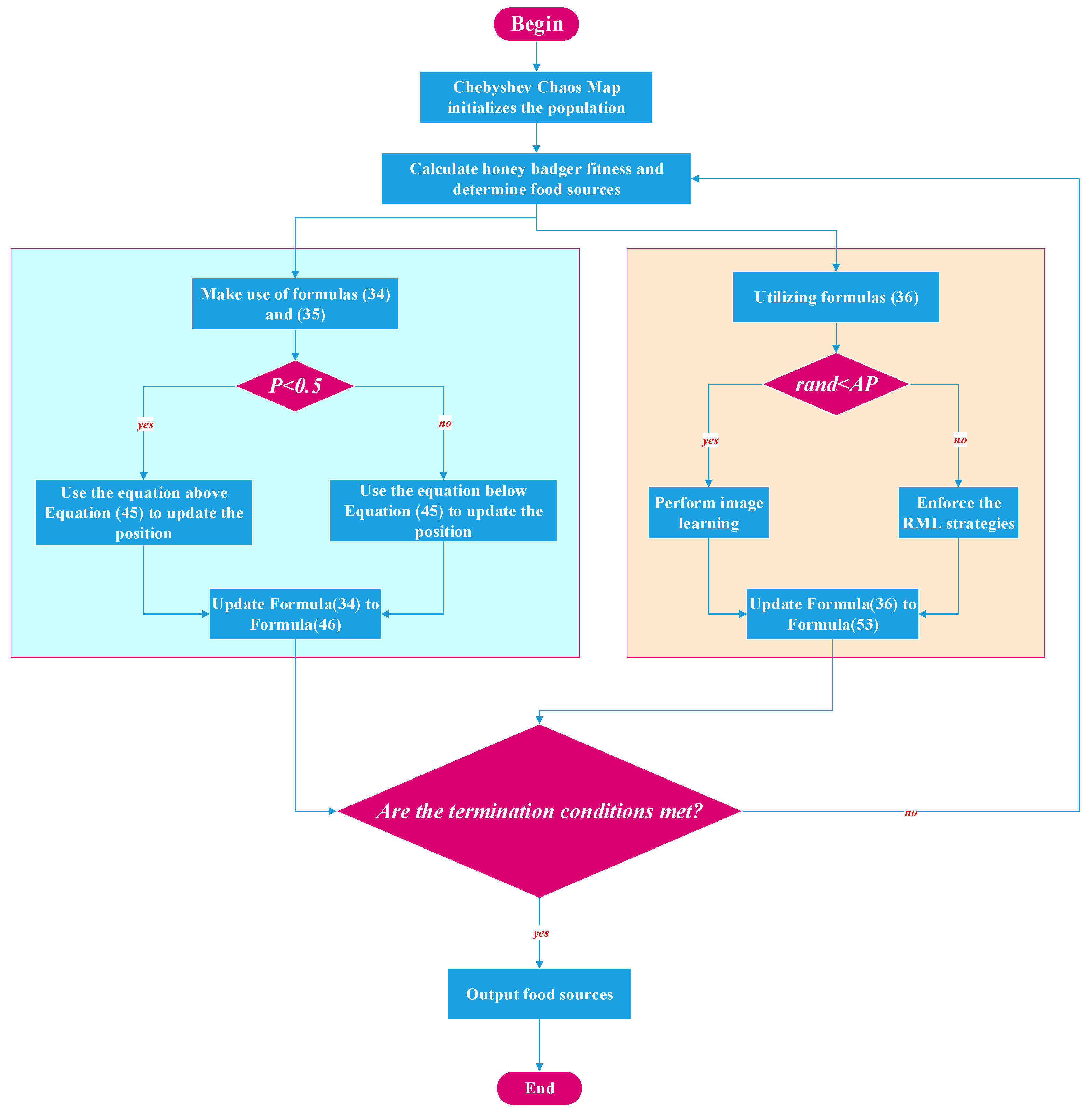
3. Improved Honey Badger Algorithm

In 2021, Fatma A. Hashim proposed a new meta-heuristic intelligent algorithm: the honey badger algorithm [31]. In order to find a food source, honey badgers will take two behaviors: sniffing and digging and following honey guide birds. The honey badger uses its olfactory ability to estimate the location of its prey, and when it gets there, it moves around its prey, choosing the right place to dig and catch its prey, a pattern that can be called a digging mode. The honey badger can also directly locate the hive under the guidance of the honey guide, which can be called the honey collection mode. This can establish the corresponding mathematical model, which is simple and easy to implement. There are few parameters to adjust; it has good application prospects and academic value. However, the local development ability of the HBA algorithm is weak, and it is difficult to jump out of the local optimization when optimizing complex problems.

In view of the problems of population diversity and unguaranteed convergence speed of swarm intelligence optimization algorithms, many scholars have carried out a lot of improved research on swarm intelligence algorithms. The authors of [32] propose a refraction learning strategy based on the principle of light refraction to optimize the whale optimization algorithm. The authors of [33] replace random parameters in the standard sine-cosine algorithm with chaotic sequences to improve the performance of the standard algorithm; ref. [34] applies the standard crow search algorithm and the particle swarm optimization algorithm with Levy flight to the finite element algorithm of simple beams; ref. [35] introduces the reverse learning strategy with refraction learning as a new operator in the algorithm to improve the searchability of the gray wolf optimization algorithm. Due to the short proposed time of HBA and relatively few improvement strategies for HBA, the above algorithm research will provide theoretical support for the improvement strategy of HBA. In view of the shortcomings of the standard HBA algorithm, this paper proposes an improved honey badger optimization algorithm based on hybrid strategy. First, in the population initialization stage, Chebyshev chaos mapping is used to maintain the diversity of the population and the superiority of the population distribution. Secondly, the refraction mirror learning strategy is integrated in the honey picking stage to find better candidate solutions while enhancing the diversity of algorithms. Finally, in the optimal individual determination stage, the moth fire fighting strategy and the golden sinusoidal strategy are introduced to update the search space of the honey badger in the exploration stage, so as to enhance the global exploration ability of the algorithm. Eleven standard test functions were selected to verify the performance of the improved HBA algorithm, and the optimization results of unimodal and multimodal and composite functions were compared and analyzed with various optimization algorithms.

3.1. Honey Badger Algorithm

3.1.1. Population Initialization Phase

Population initialization randomly initializes the number (population size) and individual location of honey badgers within a set boundary, as shown in Equation (29):

$$x_i=l{b}_i+r_1\times \left(u{b}_i+l{b}_i\right)$$

(29)

where $r_1$ is a random number within $\left(0,1\right)$; $x_i$ is the position of the i-th individual of $N$ candidates; $l{b}_i$ represents the lower bound of the search area and $u{b}_i$ represents the upper bound of the search area.

3.1.2. Define the Density Factor

Olfactory intensity is related to the concentration of prey and the distance between prey and the honey badger. The intensity of smell and the concentration of prey are related to the distance between the prey and the honey badger. The greater the olfactory intensity, the faster the honey badger moves, and the smaller the olfactory intensity, the slower the honey badger’s movement speed, given by the inverse square law, as shown in Figure 2. As shown in Equations (30)–(32):

$$I_i=r_2\times \frac{S}{4\pi d_i^2}$$

(30)

$$S={\left(x_i-x_{i+1}\right)}^2$$

(31)

$$d_i=x_{prey}-x_i$$

(32)

where $I_i$ represents the olfactory intensity of the honey badger, and $S$ is the source intensity or concentration intensity; $d_i$ represents the distance between the prey and the current honey badger individual, and $r_2$ is a random number between 0 and 1.

3.1.3. Update the Density Factor

Density factor $\alpha$ ensures a smooth transition from exploration to mining. The decreasing factor $C$ decreases with the number of iterations, updated using the method in Equation (33) to reduce the uncertainty caused by the time-varying changes in simulated honey badger foraging.

$$\alpha =C\times \exp \left(\frac{-t}{t_{\max }}\right)$$

(33)

where $t$ is the maximum number of iterations; $C$ generally defaults to 2.

3.1.4. Jump out of the Local Optimal

This and the next two steps will be used to escape the locally optimal region. In this case, the proposed algorithm uses a flag $F$, which changes the direction of the search and provides the honey badger with a higher opportunity to search for food within the space.

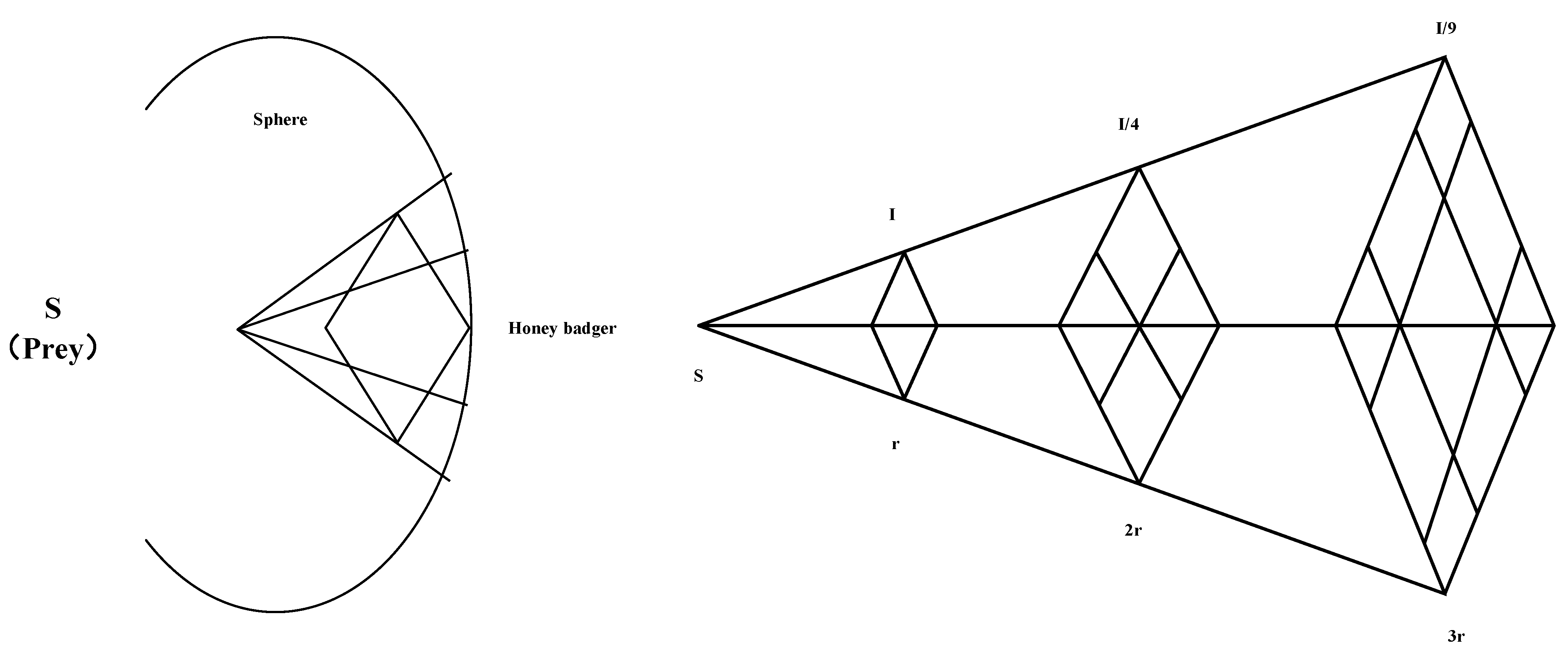
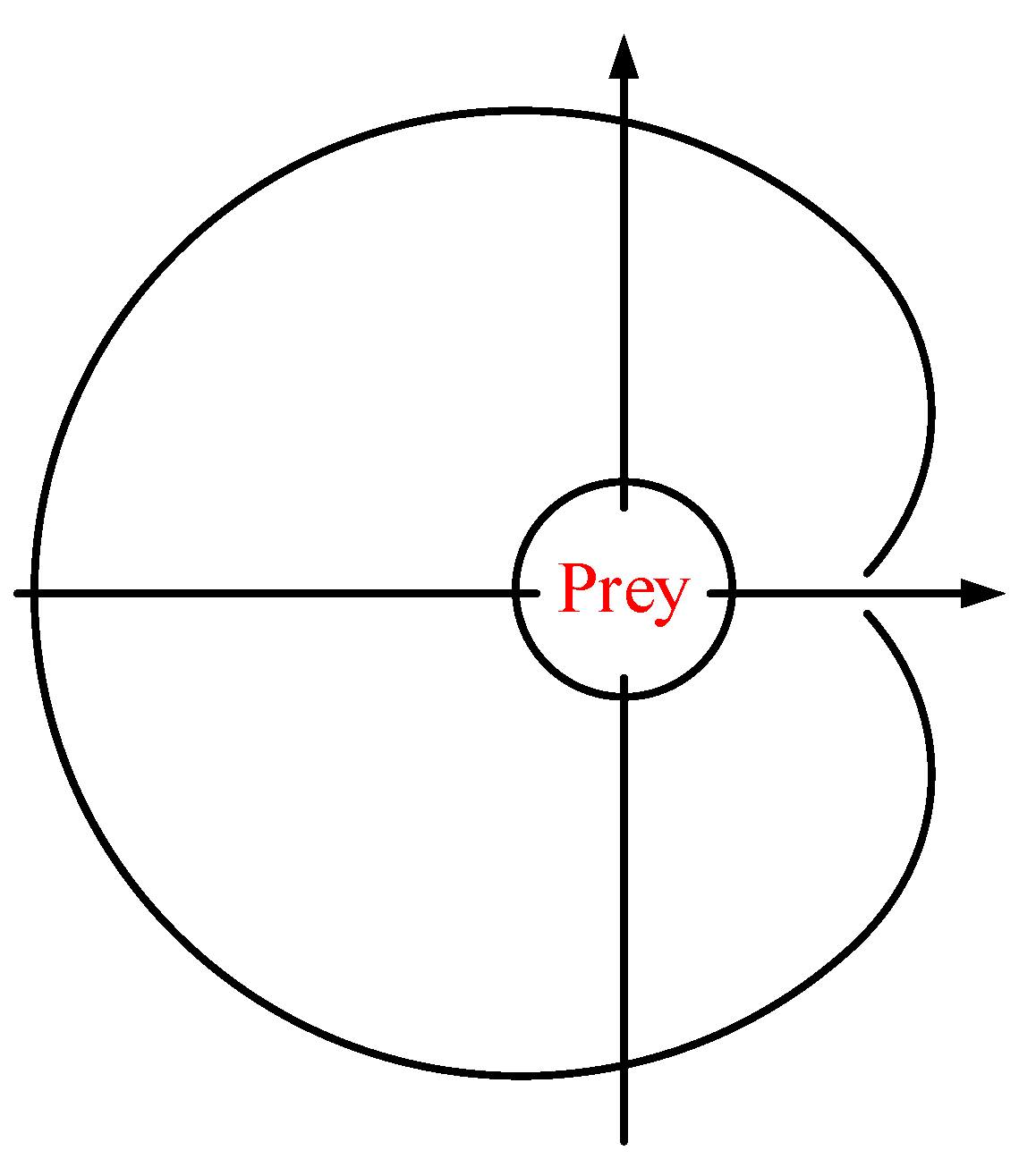
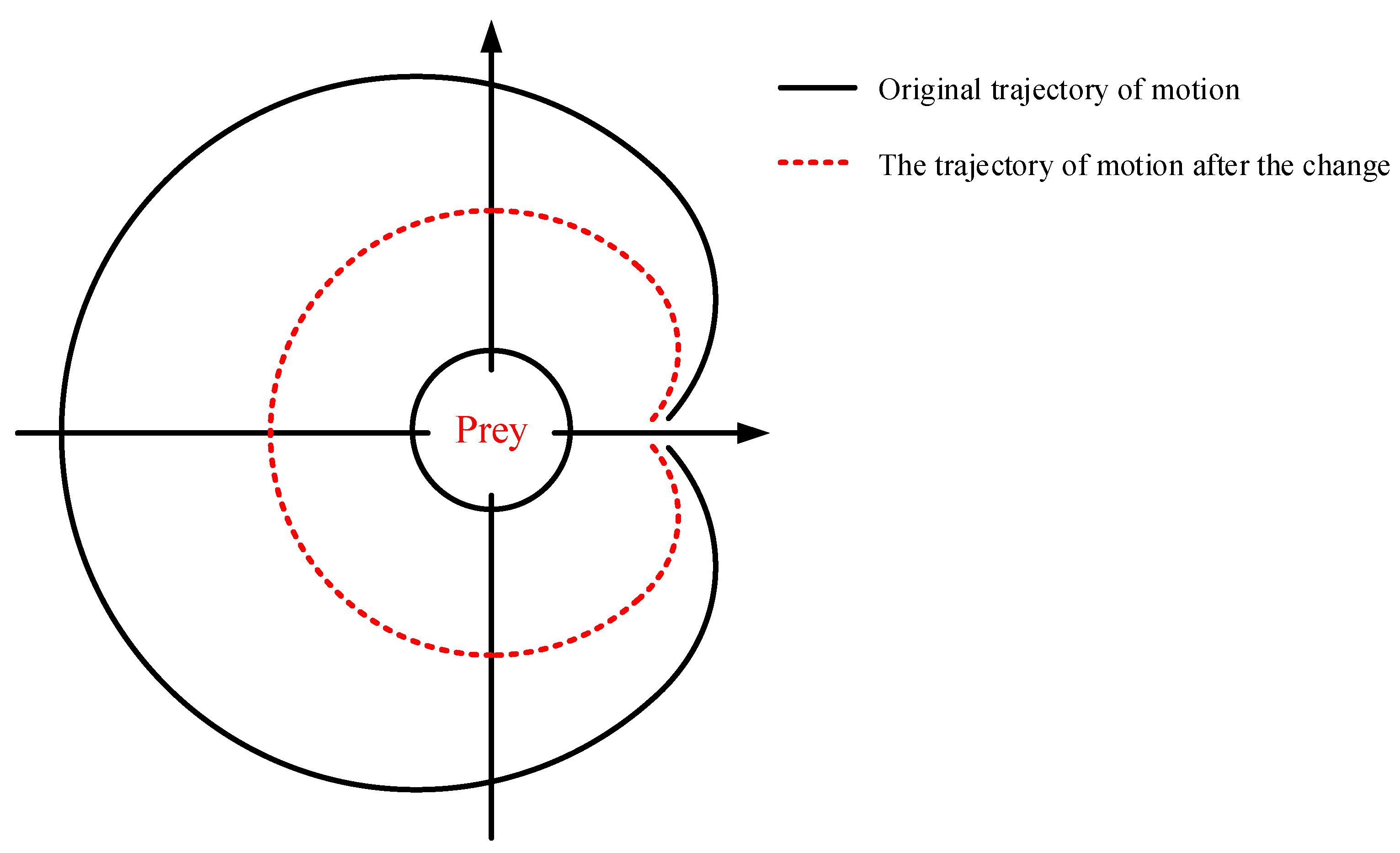
3.1.5. Excavation Phase

During the excavation phase, the honey badger performs actions similar to the shape of the heartline, as shown in Figure 3. The cardioid motion can be simulated by Equation (34):

$$x_{new}=x_{prey}+F\times \beta \times I\times x_{prey}+F\times r_3\times \alpha \times d_i\times \left|\cos \left(2\pi r_4\right)\times \left[1-\cos \left(2\pi r_5\right)\right]\right|$$

(34)

where x_prey is the global optimal position in the current state; β (generally defaulted to 6) is the ability of the honey badger to obtain food, and $d_i$ is the distance between the prey and the current honey badger individual; $r_3$, r₄, $r_5$ are three different random numbers between $\left(0,1\right)$; $F$ is a flag that changes the direction of the search, using Equation (35) to determine:

$$F=\{\begin{array}{cccc}1& & if& r_6<0.5\\ -1& & else& \end{array}$$

(35)

During the excavation phase, honey badgers rely heavily on the odor intensity of the prey, the distance from the prey, and the time-varying search influence factor. In addition, during excavation activities, honey badgers may be subjected to various disturbances, which prevent them from finding a better prey position.

3.1.6. Honey Picking Stage

The situation that the honey badger follows the honey guide bird to the hive or the movement trajectory of the honey source can be simulated by Equation (36):

$$x_{new}=x_{prey}+F\times r_7\times \alpha \times d_i$$

(36)

Among them, $x_{new}$ is the updated individual position of the honey badger; $x_{prey}$ is the prey position; $F$ and $\alpha$ are determined by Equations (35) and (33), respectively; $r_7$ is a random number between $\left(0,1\right)$. As can be seen from Equation (36), according to the distance information $d_i$, the honey badger searches near the prey location $x_{prey}$.

3.2. Improve Policies

3.2.1. Chebyshev Chaos Mapping

At present, the chaos map used in the swarm intelligence algorithm is used to initialize the population, and there are many kinds of chaos, which mainly use logistic chaos mapping, tent chaos mapping, etc., but logistic mapping is sensitive to initial parameters and has poor transversality, and the chaotic sequence of tent mapping has shortcomings in small periods, uncertain period points, etc. In summary, Chebyshev chaos mapping [36] is used to initialize a more uniform initial population; compared with tent mapping and logistic mapping, Chebyshev chaos mapping has simpler mathematical expressions, which helps the algorithm converge better, as defined in Equation (37).

$$p^{i+1}=\cos \left(i {\cos }^{-1}\left(p^i\right)\right)$$

(37)

In the above equation, $p$ is the random number of the interval $\left[-1,1\right]$ and $i$ is the order. The steps to initialize the honey badger population are as follows:

• Initialize the honey badger population $N$ and initialize the spatial position of the first body in $D$-dimensional space, $Z=\left\{z_1,z_2,\cdot \cdot \cdot ,z_i,\cdot \cdot \cdot ,z_D\right\},z_i\in \left[-1,1\right]$;
• Equation (37) is used to change each dimension $x_i$ of individual $X$ from generation to generation, new until the remaining $N-1$ honey badger individuals are spawned.
• Further mapping to the initial location of the honey badger individual in the search space:

  $$X_j^i=l{b}_i+\left(1+Z_j^i\right)\times \frac{\left(u{b}_i-l{b}_i\right)}{2}$$

  (38)

  where $ub$ and $lb$ are the upper and lower bounds of the search space, $j\in \left[1,N\right]$.

3.2.2. Mix Golden Sine with Moth-Flame Operator

The Golden Sine Algorithm [37] is a meta-heuristic proposed by Tanyildizi et al. in 2017, which iterates through all points on the unit circle, that is, all points on the sinusoidal function, based on the relationship between the unit circle and the sinusoidal function. The moth-flame optimization algorithm [38] is a new swarm intelligence algorithm proposed by Mirjalili et al. in 2015, which proposes a new spiral search method to optimize the position of flames. Combine the two strategies to enhance the algorithm’s global exploration capabilities.

Gold-SA introduces the golden ratio coefficients $c_1$ and $c_2$ into the slash solution space in the position update, thereby balancing exploration and development capabilities, mathematically expressed as follows:

$$c_1=-\pi +2\pi \left(1-\tau \right)$$

(39)

$$c_2=-\pi +2\pi \tau$$

(40)

where $\tau$ is the gold split ratio, fetched $\tau =\frac{\left(\sqrt{5}-1\right)}{2}\approx 0.6183$.

The golden section coefficient cuts the solution space once per iteration, and the position update formula is as follows:

$$x_{enew}=x_{new}{}^{\prime }\left|\sin \left({\phi }_1\right)\right|-{\phi }_2\sin \left({\phi }_1\right)\left|c_1{F}^{\prime }-c_2{x}_i\right|$$

(41)

Thereinto, $x_{new}{}^{\prime }$ is the current location of the honey badger, random numbers within ${\phi }_1\in \left(0,2\pi \right)$, random numbers within ${\phi }_2\in \left(0,\pi \right)$, $F^{\prime }$ is the position of the new prey.

In the moth-flame optimization algorithm, the positions of moths and flames are represented by matrices, and the fitness values of moths and flames are represented by vectors, which are sorted by the size of the fitness values. The spiral flight update formula for moths in the moth-flame optimization algorithm is as follows:

$$S\left(M_i,F_j\right)=D_i\cdot e^{bt}\cdot \cos \left(2\pi t\right)+F_j$$

(42)

$$D_i=\left|F_j-M_i\right|$$

(43)

where $M_i$ is the position of the $i$th moth, $F_j$ is the position of the $j$th flame, $D_i$ is the distance between the moth and the flame in the current iteration, $b$ is the logarithmic spiral coefficient; in this case, it is 1. After updating the position of the moth at the end, use Equation (44) to reduce the number of flames with the iteration.

$$flame no=round\left(N-L\cdot \frac{N-1}{T}\right)$$

(44)

where $N$ is the maximum number of flames, $L$ is the number of current iterations, $T$ is the maximum number of iterations. As the iteration progresses, the number of flames gradually decreases, and at the end of the iteration, the moth only updates the position according to the optimal flame position.

Therefore, in this paper, the Gold-SA algorithm is transplanted as a local operator, and the position update formula in the mining stage is introduced, so that the optimization space is reduced, the optimization time is reduced, and the convergence speed is accelerated. Then, the spiral flight of moths to the fire is applied as an operator to the bubble net search mechanism of the whale optimization algorithm [39], which has certain portability. The improved Equation (45) is as follows:

$$x_{new}=\{\begin{array}{c}{x}_{prey}+F\times \beta \times I\times x_{prey}+F\times r_3\times \alpha \times {d_i}^{\prime }\times \left|\cos \left(2\pi r_4\right)\times \left[1-\cos \left(2\pi r_5\right)\right]\right|\times x_{enew}\begin{array}{cc}& p<0.5\end{array}\\ d_i{}^{\prime }\cdot e^{bt}\cdot \cos \left(2\pi t\right)+F^{\prime }\begin{array}{cc}& p\ge 0.5\end{array}\end{array}$$

(45)

where $d_i{}^{\prime }$ is the distance between the current iteration honey badger and its prey, $b$ is the coefficient of the spiral.

By introducing two optimization algorithms, the mining and search mechanism of the honey badger algorithm is fundamentally changed, and the search space of the honey badger in the exploration stage is reduced under the condition that the prey range remains unchanged, which greatly shortens the time for the honey badger to seek excellence, as shown in Figure 4.

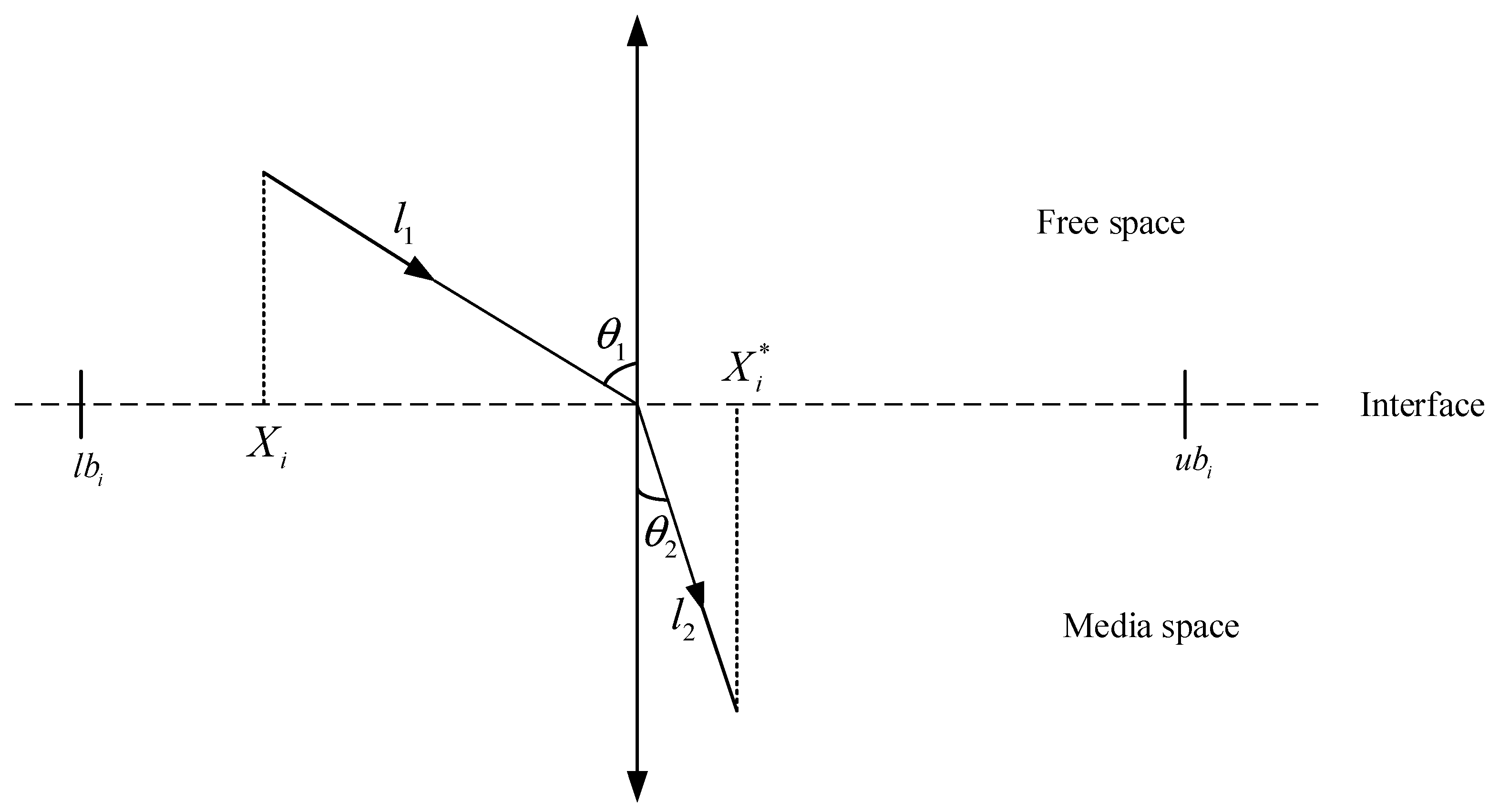
3.2.3. Refraction Mirror Learning Strategy

In recent years, in the study of intelligent algorithms, many scholars have used the reverse learning method, which will generate the reverse solution of the feasible solution and select a better candidate solution for the evaluation of the reverse solution. The difference between mirror learning [39] and reverse learning [40] to be integrated in this paper is that the mirror learning strategy is to use the mirror image of light to achieve the overall mutation of the population. Refraction mirror learning strategy combines the law of refraction of light and the image selection characteristics to summarize an improved strategy, which can enhance the diversity of algorithms to find better candidate solutions. The refractive mirror learning strategy is shown in Figure 5.

Suppose that in the natural space region, let the angle between the angle of incidence and normal $n$ be ${\theta }_1$, the angle between the exit angle and the normal $n$ be ${\theta }_2$, and the lengths of the incident ray and the outgoing ray are $l_1$ and $l_2$, respectively. By the law of refraction:

$$n_0\sin \left({\theta }_1\right)=n_1\sin \left({\theta }_2\right)$$

(46)

where $n_0$ is the refractive index of free space, usually 1. $n_1$ is the refractive index of the medium, usually $n_1>1$. By geometric relations:

$$\sin \left({\theta }_1\right)=\frac{\left(u{b}_i+l{b}_i\right)/2-x}{l_1}$$

(47)

$$\sin \left({\theta }_2\right)=\frac{X_i^{\ast }-\left(u{b}_i+l{b}_i\right)/2}{l_2}$$

(48)

Combined with the law of refraction, the length of the incident ray and the length of the outgoing ray $k=l_1/l_2$ are integrated:

$$k{n}_1=\frac{\left(u{b}_i+l{b}_i\right)/2-x}{X_i^{\ast }-\left(u{b}_i+l{b}_i\right)/2}$$

(49)

The reverse solution $X_i^{\ast }$ yields:

$$X_i^{\ast }=\frac{u{b}_i+l{b}_i}{2}+\frac{u{b}_i-l{b}_i-2X_i}{2k{n}_1}$$

(50)

When $k=n_1=1$, there are:

$$X_i^{\ast }=u{b}_i+l{b}_i-X_i$$

(51)

Obviously, when $k$ and $n_1$ are 1, Equation (44) is only a special case of refractive mirror learning, and the way of candidate solutions is relatively fixed. The RML can adjust the parameters according to different values to obtain dynamic candidate solutions, which increases the probability of the algorithm jumping out of the local optimal.

In order to enhance the search diversity of solutions and improve the optimization ability, the image learning and RML strategies are alternately executed with a certain probability, so that the candidate solutions can be dynamically updated with the parameters, which not only retains the advantages of image learning, but also gives full play to the advantages of RML. In this topic, the segmented search expressions are as follows:

$$X_i^{\ast }=\{\begin{array}{l}u{b}_i+l{b}_i-X_i\hspace{1em}\hspace{1em}\hspace{1em}rand<AP\\ \frac{u{b}_i+l{b}_i}{2}+\frac{u{b}_i+l{b}_i-2X_i}{2k{n}_1}\hspace{1em}rand\ge AP\end{array}$$

(52)

In Equation (45), $AP$ is the probability of selecting a threshold, generating random numbers higher than $AP$ and choosing RML, and below $AP$ selecting mirror learning. After many independent experiments, $AP=0.35$ has the best optimization effect.

Therefore, this paper will introduce the individual position update formula of honey badgers in the honey picking stage with mirror learning and RML strategies that are executed alternately with a certain probability, so that better candidate solutions can be found while enhancing the search diversity of the algorithm and improving the optimization ability. The improved Equation (53) is as follows:

$$x_{new}=x_{prey}+F\times r_7\times \alpha \times d_i\times X_i^{\ast }$$

(53)

The pseudo code for IHBA is as follows Algorithm 1:

Algorithm 1 Pseudo code of IHBA.

$\mathrm{Set} \mathrm{parameters} t_{\max }$, $N$, $\beta$, $C$, $\mathrm{and} \mathrm{search} \mathrm{space} \mathrm{lower} \mathrm{bound} lb$$\mathrm{and} \mathrm{upper} \mathrm{boundary} ub$.

Initialize population with random positions.

$\mathrm{Initialize} \mathrm{population} x_i$ using Chebyshev chaos mapping.

$\mathrm{Evaluate} \mathrm{the} \mathrm{fitness} \mathrm{of} \mathrm{each} \mathrm{honey} \mathrm{badger} \mathrm{position} x_i$ using objective function.

$\mathrm{Save} \mathrm{best} \mathrm{position} x_{prey}$.

while $t\le t_{\max }$ do

Update the decreasing factor $\alpha$ using Equation (33).

for i = 1 to N do

$\mathrm{Calculate} \mathrm{the} \mathrm{intensity} I_i$ using Equation (32).

if $r<0.5$ then

$\mathrm{Update} \mathrm{the} \mathrm{position} x_{new}$ using Equation (34).

if $p<0.5$ then

$\mathrm{Use} \mathrm{the} \mathrm{equation} \mathrm{above} \mathrm{Equation} \left(45\right) \mathrm{to} \mathrm{update} \mathrm{the} \mathrm{position} x_{new}$.

else

$\mathrm{Use} \mathrm{the} \mathrm{equation} \mathrm{below} \mathrm{Equation} \left(45\right) \mathrm{to} \mathrm{update} \mathrm{the} \mathrm{position} \mathrm{of} x_{new}$.

end if

else

$\mathrm{Update} \mathrm{the} \mathrm{position} x_{new}$ using Equation (36).

if $rand<AP$ then

Perform image learning.

else

Enforce the RML strategies.

end if

for $AP=0.35$ do

$\mathrm{Update} \mathrm{the} \mathrm{position} x_{new}$ using Equation (53).

end for

end if

end for

end while Stop criteria satisfied.

Return $x_{prey}$

The flowchart here is Figure 6.

3.3. Simulation Experiments and Results Analysis

3.3.1. Function Selection and Parameter Setting

This paper uses MATLAB R2018a for experimental simulation. The operating environment is a 64-bit Windows 10 operating system, and the processor type is Intel Core i7-6700 HQ CPU @ 2.60 GHz, Win10 PC.

In order to verify the performance of the proposed algorithm and verify the correlation between the strategies proposed in this paper [41], the honey badger algorithm (IHBA) proposed in this paper is compared with the traditional honey badger algorithm (HBA), butterfly optimization algorithm (BOA), particle swarm algorithm (PSO), sine cosine algorithm (SCA), bottle sea squirt algorithm (SSA), whale optimization algorithm (WOA), and dragonfly optimization algorithm (DA), and 11 classical functions with different optimization characteristics are introduced as shown in

Table 1. Test functions.

Function Name	Function Formulas	Dimension	Search Compartments	Theoretical Value	Function Type
Sphere	$F_1(X)={\displaystyle \sum _{i=1}^n{x}_i^2}$	20	[−100, 100]	0	Unimodal
Schwefel’s 2.22	$F_2(X)={\displaystyle \sum _{i=1}^n\left|x_i\right|}+{\displaystyle \prod _{i=1}^n\left|x_i\right|}$	100	[−10, 10]	0	Unimodal
Schwefel’s 1.2	$F_3(X)={\displaystyle \sum _{i=1}^n({\displaystyle \sum _{j=1}^i{x}_j}}{)}^2$	10	[−100, 100]	0	Unimodal
Schwefel’s 2.21	$F_4(X)=\max \left\{\left|x_j\right|\right\}$	60	[−100, 100]	0	Unimodal
Rosenbrock’s	$F_5(X)=[100{(x_{i+1}-x_i^2)}^2+{(1-x_i)}^2]$	30	[−30, 30]	0	Unimodal
Step	$F_6(X)={{\displaystyle \sum _{i=1}^n(\lfloor x_i+0.5\rfloor )}}^2$	30	[−100, 100]	0	Unimodal
Quartic	$F_7(X)={\displaystyle \sum _{i=1}^{n}i{x}_i^4+random[0,1)}$	10	[−1.28, 1.28]	0	Unimodal
Rastrigin	$F_8(X)={\displaystyle \sum _{i=1}^n[x_i^2-10\cos (2\pi x_i)+10]}$	200	[−5.12, 5.12]	0	Multimodal
Ackley	$F_9(X)=-20\exp (-0.2\sqrt{{\displaystyle \sum _{i=1}^n{x}_i^2/n}})-\exp ({\displaystyle \sum _{i=1}^n\cos (2\pi x_i/n)+20+e}$	50	[−32, 32]	0	Multimodal
Girwank	$F_{10}(X)=\frac{1}{4000}{\displaystyle \sum _{i=1}^n{x}_i^2}-{\displaystyle \prod _{i=1}^n\cos \left(\frac{x_i}{\sqrt{i}}\right)}+1$	20	[−600, 600]	0	Multimodal
Penalized	$F_{11}(X)=4x_1^2-2.1x_1^4+x_1^6/3+x_1{x}_2-4x_2^2+4x_2^4$	30	[−50, 50]	0	Multimodal

. Since F1~F7 is a unimodal function, the local optimal is the global optimal, which is used to test the convergence speed and convergence accuracy of the IHBA algorithm proposed in this paper. Among them, F8~F11 is a multimodal function, with multiple local extremums; especially the variables of F9 and F10 are related to each other, making it difficult for the algorithm to search for the global optimum, which is used to test the ability of the algorithm to jump out of the local optimum. In the experiment, 30 independent runs will be used to test the algorithm performance, where the population number is 30 and the maximum number of iterations is 500. In addition, the dimension of the test function is also a key factor affecting algorithm optimization, so the dimensions of the test function listed in Table 1 range from 10 to 200, which can verify the algorithm performance more comprehensively.

The 11 benchmark functions in the lab are shown in Table 1. The basic parameters of each algorithm in the experiment are shown in

Table 2. Factor of functions.

Algorithm	Main Parameter Settings
IHBA	$C=2, \beta =6$
HBA	$C=2, \beta =6, p\in \left[-1, 1\right], n_0=1$, $k=n_1=1$
BOA	p = 0.8, c = 0.01, a = 0.1
PSO	$a_1=a_2=1.5$
SCA	$a=2$
SSA	-
WOA	$b=1$
DA	-

.

The data results of the IHBA algorithm compared with other traditional algorithms proposed in this paper are shown in

Table 3. Comparison of results of different algorithms.

	Algorithm	Function Optimum	Function Worst	Function Average	Standard Deviation	Time Elapsed
F1	IHBA	0	0	0	0	0.2688
	HBA	2.84 × 10−209	3.10 × 10−217	8.32 × 10−208	0	0.2778
	BOA	1.64 × 10−14	2.02 × 10−14	1.81 × 10−14	1.01 × 10−15	0.0942
	PSO	9.18 × 10−8	2.07 × 10−10	2.31 × 10−6	5.89	0.0549
	SCA	2.21 × 10−6	1.47	1.21 × 10−1	3.51 × 10−1	0.1147
	SSA	6.28 × 10−9	2.11 × 10−8	1.21 × 10−8	3.14 × 10−9	0.1259
	WOA	1.20 × 10−167	1.20 × 10−151	1.10 × 10−152	2.80 × 10−152	0.05088
	DA	4.45 × 102	2.37 × 103	1.04 × 103	4.36 × 102	18.927
F2	IHBA	0	0	0	0	0.2622
	HBA	6.02 × 10−106	3.99 × 10−108	8.54 × 10−105	1.69 × 10−105	0.2938
	BOA	9.89 × 10−12	1.22 × 10−11	1.10 × 10−11	6.09 × 10−13	0.1013
	PSO	9.41	2.23 × 101	1.50 × 101	3.10	0.0584
	SCA	1.26 × 10−4	7.81 × 10−9	1.26 × 10−4	4.15 × 10−4	0.1166
	SSA	7.17 × 10−3	3.25	8.28 × 10−1	8.28 × 10−1	0.1258
	WOA	3.70 × 10−115	1.20 × 10−100	3.80 × 10−102	2.10 × 10−101	0.0530
	DA	2.89 × 10−1	2.17 × 101	1.12 × 101	4.89	21.807
F3	IHBA	0	0	0	0	0.4797
	HBA	6.65 × 10−200	2.77 × 10−209	2.00 × 10−198	0	0.5254
	BOA	1.63 × 10−14	2.09 × 10−14	1.82 × 10−14	1.05 × 10−15	0.4253
	PSO	8.36 × 101	2.78 × 102	1.74 × 102	4.75 × 101	0.2191
	SCA	1.69 × 102	1.10 × 104	3.48 × 103	2.93 × 103	0.2765
	SSA	7.27 × 101	6.78 × 102	2.67 × 102	1.50 × 102	0.2956
	WOA	4.86 × 103	4.38 × 104	2.17 × 104	9.53 × 103	0.2192
	DA	2.57 × 103	2.12 × 104	1.15 × 104	5.54 × 103	22.809
F4	IHBA	0	0	0	0	0.2321
	HBA	1.43 × 10−102	5.14 × 10−107	2.96 × 10−101	5.68 × 10−102	0.2428
	BOA	1.10 × 10−11	1.38 × 10−11	1.22 × 10−11	6.47 × 10−13	0.0959
	PSO	1.99	2.88 × 102	2.43	2.22 × 10−1	0.0570
	SCA	1.59	3.95 × 101	1.91 × 101	1.05 × 101	0.1125
	SSA	2.93	1.55 × 101	8.70	3.45	0.1282
	WOA	5.40 × 10−2	8.95 × 101	3.70 × 101	3.04 × 101	0.0561
	DA	1.38 × 101	3.58 × 101	2.25 × 101	5.99	16.682
F5	IHBA	2.66 × 101	2.56 × 101	2.73 × 101	1.13 × 10−3	0.2752
	HBA	2.88 × 101	2.84 × 101	2.89 × 101	1.20 × 10−1	0.2806
	BOA	2.89 × 101	2.90 × 101	2.89 × 101	3.00 × 10−2	0.1355
	PSO	2.16 × 103	1.48 × 104	6.07 × 103	2.92 × 103	0.0751
	SCA	2.77 × 101	8.24 × 103	5.47 × 102	1.59 × 103	0.1328
	SSA	1.81 × 101	1.79 × 103	2.41 × 102	4.20 × 102	0.1484
	WOA	2.84 × 101	2.90 × 101	2.88 × 101	1.21 × 10−1	0.4616
	DA	4.23 × 103	6.25 × 105	1.11 × 105	1.28 × 105	18.916
F6	IHBA	4.01 × 10−14	1.52 × 10−9	8.45 × 10−11	2.78 × 10−10	0.2376
	HBA	1.50 × 10−1	2.19 × 10−1	6.26	6.10 × 10−1	0.2327
	BOA	4.51	6.65	5.83	4.89 × 10−1	0.0928
	PSO	7.19	2.66 × 101	1.66 × 101	5.50	0.0558
	SCA	3.77	7.54	4.58	6.45 × 10−1	0.1110
	SSA	7.91 × 10−9	2.18 × 10−8	1.31 × 10−8	3.39 × 10−9	0.1251
	WOA	1.11 × 10−2	3.69 × 10−1	9.47 × 10−2	9.76 × 10−2	0.0515
	DA	2.89 × 102	3.76 × 103	1.09 × 103	6.41 × 103	18.836
F7	IHBA	6.82 × 10−7	1.88 × 10−4	5.71 × 10−5	4.54 × 10−5	0.2389
	HBA	2.81 × 10−4	3.26 × 10−5	1.81 × 10−3	3.54 × 10−4	0.2285
	BOA	2.28 × 10−4	1.11 × 10−3	6.57 × 10−4	2.33 × 10−4	0.2854
	PSO	2.77 × 101	1.10 × 102	5.93 × 101	2.36 × 101	0.1543
	SCA	3.46 × 10−3	2.11 × 10−1	4.06 × 10−2	4.64 × 10−2	0.2094
	SSA	4.46 × 10−2	2.13 × 10−1	1.09 × 10−1	4.30 × 10−2	0.2251
	WOA	1.17 × 10−4	1.19 × 10−2	2.22 × 10−3	2.84 × 10−3	0.1478
	DA	1.15 × 10−1	6.20 × 10−1	2.83 × 10−1	1.32 × 10−1	16.723
F8	IHBA	0	0	0	0	0.7173
	HBA	0	0	0	0	0.7798
	BOA	0.00E+00	2.04 × 102	3.16 × 101	7.20 × 10−1	0.1235
	PSO	1.70 × 102	2.70 × 102	2.17 × 102	2.89 × 101	0.0756
	SCA	3.25 × 10−5	1.44 × 102	2.25 × 101	4.13 × 101	0.1237
	SSA	2.29 × 101	8.86 × 101	6.10 × 101	1.83 × 101	0.1409
	WOA	0	0	0	0	0.0570
	DA	8.69 × 101	2.40 × 102	1.58 ×102	3.86 × 101	18.460
F9	IHBA	8.88 × 10−16	8.88 × 10−16	8.88 × 10−16	0	0.2738
	HBA	8.88 × 10−16	4.44 × 10−15	2.90 × 10−15	1.79 × 10−15	0.3914
	BOA	1.13 × 10−11	1.46 × 10−11	1.29 × 10−11	9.03 × 10−13	0.1133
	PSO	3.59	5.37	4.39	3.66 × 10−1	0.0780
	SCA	4.91 × 10−4	2.03 × 10−1	1.34 ×10−1	8.86	0.1382
	SSA	2.18 × 10−5	2.96	1.93	7.33 ×10−1	0.1437
	WOA	8.88 × 10−16	7.99 × 10−15	4.20 × 10−15	2.07 × 10−15	0.0593
	DA	0	1.18 × 10−1	5.24 × 10−3	2.24 × 10−2	0.0753
F10	IHBA	0	0	0	0	0.2535
	HBA	0	0	0	0	0.3989
	BOA	0	6.44 × 10−15	1.64 × 10−15	1.79 × 10−15	0.1459
	PSO	3.35 × 10−1	7.95 × 10−1	5.27 × 10−1	1.21 × 10−1	0.0890
	SCA	6.15 × 10−5	7.24 × 10−1	3.08 × 10−1	2.14 × 10−1	0.1446
	SSA	3.30 × 10−8	4.44 × 10−2	1.00 × 10−2	1.07 × 10−2	0.1597
	WOA	5.06	1.17	8.60	1.89	18.383
	DA	3.19	2.82 × 101	1.26 × 101	6.57	19.235
F11	IHBA	6.91 × 10−3	2.63 × 10−3	1.18 × 10−2	1.06 × 10−2	0.5501
	HBA	7.09 × 10−1	3.28 × 10−1	1.18 × 101	2.06 × 10−1	0.6714
	BOA	4.01 × 10−1	1.00	6.61 × 10−1	1.51 × 10−1	0.8359
	PSO	1.72 × 10−2	3.00 × 10−8	2.07 × 10−1	4.78 × 10−2	0.3696
	SCA	5.78 × 10−1	1.44 × 106	6.86 × 104	2.66 × 105	0.4443
	SSA	1.59	1.86 × 101	7.33	3.40	0.4133
	WOA	2.31 × 10−2	6.16 ×10−3	9.91 × 10−2	1.98 × 10−2	0.3538
	DA	1.34 × 103	5.67	2.36 × 104	4.76 × 103	25.125

.

It can be seen from Table 3 that, compared with other traditional swarm intelligence optimization algorithms, the performance of the IHBA algorithm on the four unimodal functions F1 to F4 is much higher than that of other traditional swarm intelligence algorithms, and its optimization has reached the optimal value, its optimization stability is good, and there is no phenomenon that the individual optimization value deviates from the theoretical value in 30 experiments. On the three unimodal functions of F5, F6, and F7, although the IHBA algorithm does not find the theoretical value of the test function, the optimization accuracy is at least two orders of magnitude higher than that of the traditional HBA algorithm, SCA and SSA, and the improved algorithm proposed in this paper can also be equal to the optimization accuracy compared with the BOA with better optimization performance. On the two multimodal functions F8 and F10, the IHBA algorithm can also find the theoretical value of the test function; it is worth noting that although the dimension of the function F8 is 200 dimensions, the IHBA algorithm is not affected too much, and while finding the theoretical value, the standard deviation of the 30-time data is 0, that is, its optimization process is very stable. On the two multimodal functions of F9 and F11, although the IHBA algorithm does not search the theoretical value of the algorithm, it has a great improvement compared with several other traditional algorithms, among which is the F9 function. In each of the 30 experiments, the local optimal value of 8.88 × 10⁻¹⁶ fell into the late iteration, and its optimization accuracy was improved by 16 orders of magnitude compared with other traditional algorithms except WOA and BOA, which were improved by 2 and 5 orders of magnitude, respectively, compared to WOA and BOA, and at least 7 orders of magnitude higher in F11 functions than other algorithms other than BOA, and 2 orders of magnitude higher for BOA. In summary, although the IHBA algorithm improves the accuracy and stability of each test function differently than other traditional swarm intelligence algorithms, in general, the IHBA algorithm has certain advantages in solving various benchmark functions.

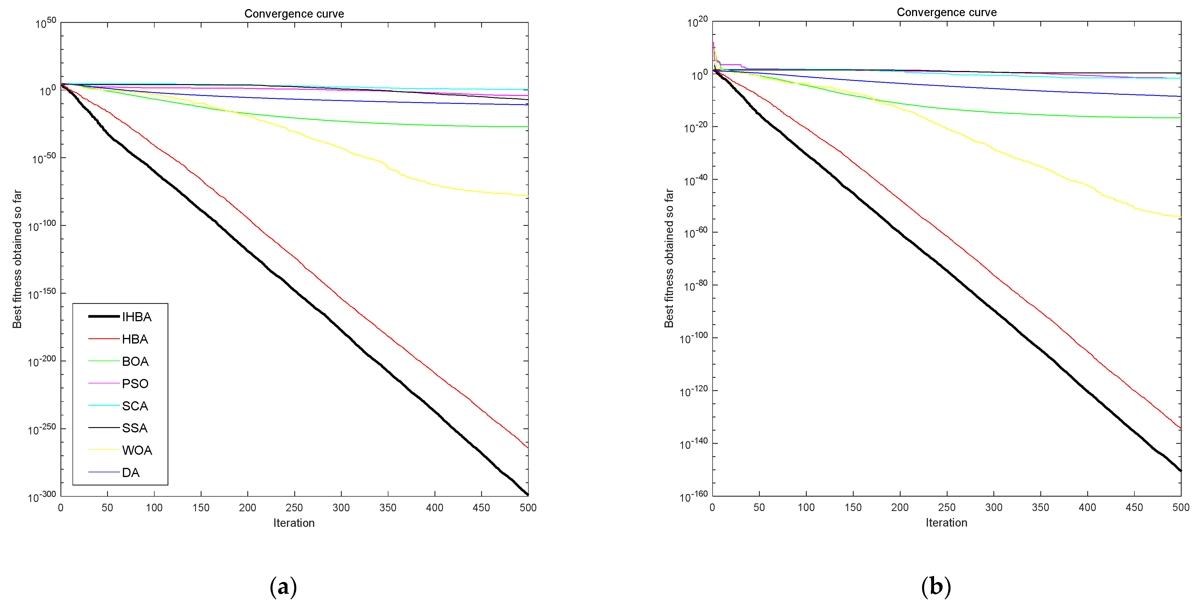
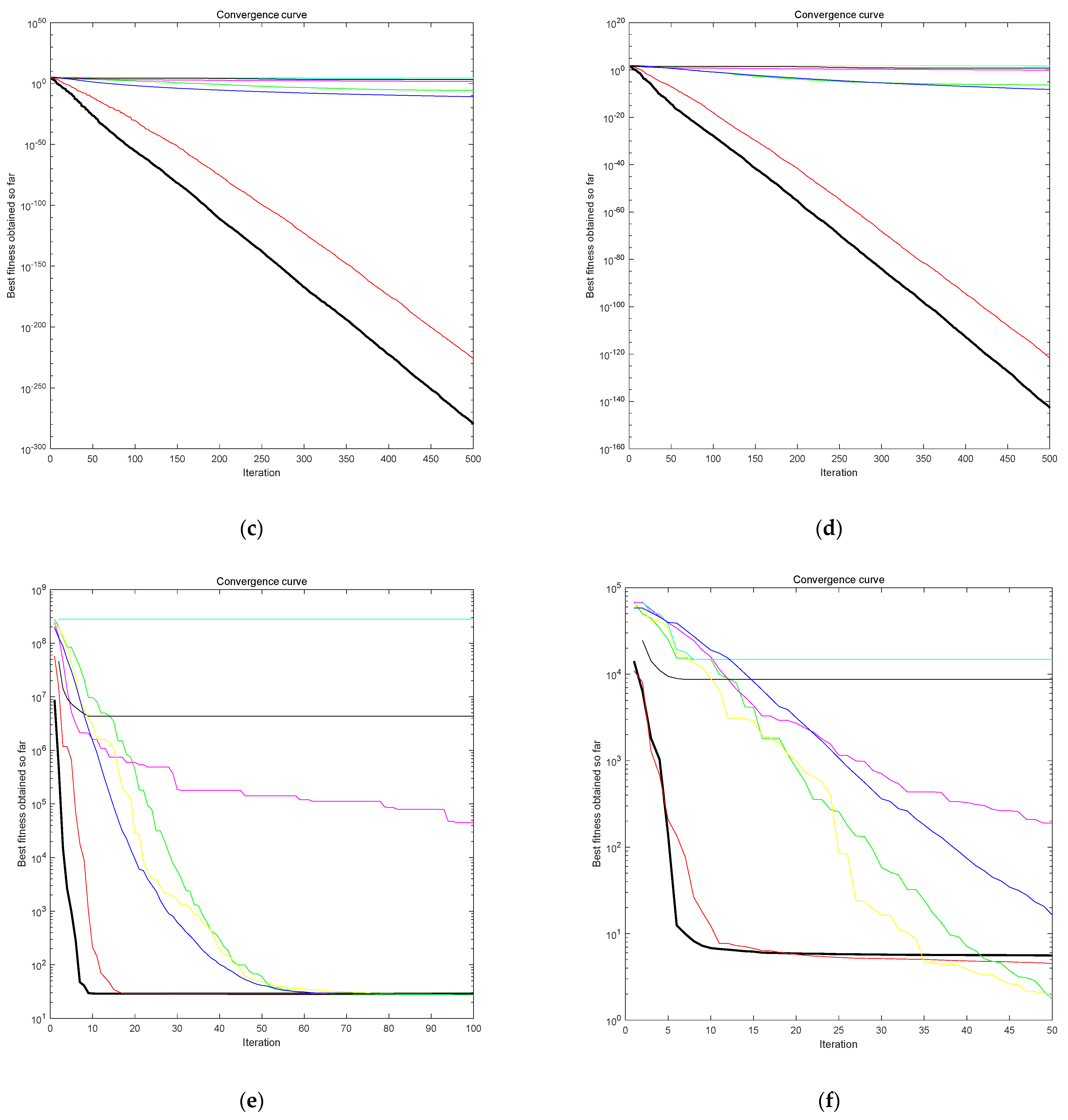
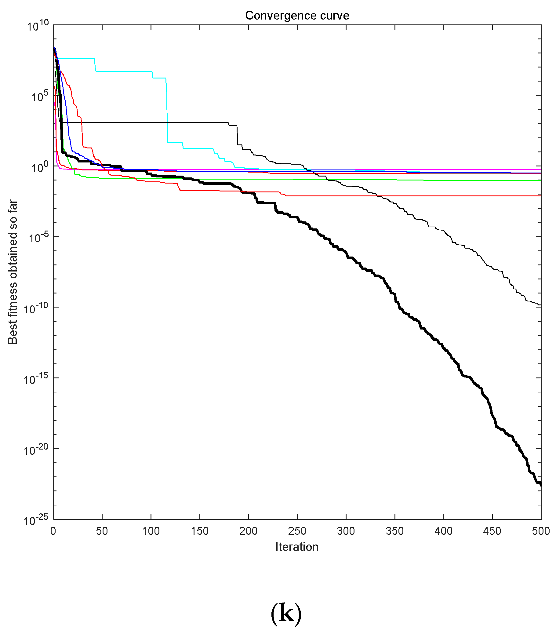
3.3.2. Test the Function Convergence Curve

According to the experimental data, the average convergence curve of 11 test functions of each algorithm and strategy running independently 30 times is shown in Figure 7.

3.3.3. Wilcoxon Rank Sum Test

Although the mean and standard deviation obtained in 30 independent experiments have certain reference significance, in multiple experiments, there may be a situation where the effect of an experiment is extremely good or very poor, which is when the mean and standard deviation of experimental data can not be reflected, so when evaluating the performance of the improved algorithm, it is not enough to rely only on the mean and standard deviation, and statistical tests are carried out to prove that the improved algorithm proposed in this paper is very necessary. At 5%, Wilcoxon rank sum test [42] is performed at the significance level to determine that the IHBA algorithm has significant performance improvement on some specific problems.

Table 4. p-Values of Wilcoxon rank sum test of test function.

Algorithm	HBA		BOA		PSO		SCA		SSA		WOA		DA
	P	S	P	S	P	S	P	S	P	S	P	S	P	S
F1	1.18 × 10−12	+	1.21 × 10−12	+	1.21 × 10−12	+	1.16 × 10−13	+	1.04 × 10−12	+	1.21 × 10−12	+	7.95 × 10−13	+
F2	1.08 × 10−12	+	1.21 × 10−12	+	1.11 × 10−12	+	1.53 × 10−12	+	4.91 × 10−13	+	1.21 × 10−12	+	7.33 × 10−13	+
F3	1.04 × 10−12	+	1.21 × 10−12	+	1.17 × 10−12	+	2.80 × 10−12	+	3.11 × 10−12	+	1.05 × 10−12	+	3.77 × 10−13	+
F4	1.15 × 10−12	+	1.21 × 10−12	+	1.21 × 10−12	+	1.17 × 10−13	+	4.91 × 10−13	+	5.35 × 10−13	+	3.16 × 10−13	+
F5	2.92 × 10−11	+	3.02 × 10−11	+	2.92 × 10−11	+	4.56 × 10−11	+	3.02 × 10−11	+	3.02 × 10−11	+	2.05 × 10−11	+
F6	2.99 × 10−11	+	3.02 × 10−11	+	3.02 × 10−11	+	1.20 × 10−10	+	1.72 × 10−10	+	3.02 × 10−11	+	2.60 × 10−11	+
F7	2.92 × 10−11	+	3.02 × 10−11	+	9.31 × 10−12	+	4.56 × 10−11	+	2.01 × 10−10	+	2.89 × 10−11	+	2.61 × 10−11	+
F8	1.17 × 10−12	+	9.23 × 10−13	+	6.81 × 10−13	+	1.17 × 10−13	+	1.27 × 10−12	+	1.20 × 10−12	+	4.17 × 10−13	+
F9	1.19 × 10−12	+	1.11 × 10−12	+	1.19 × 10−12	+	2.36 × 10−11	+	8.75 × 10−12	+	1.21 × 10−12	+	6.29 × 10−13	+
F10	1.16 × 10−12	+	1.21 × 10−12	+	1.10 × 10−12	+	1.17 × 10−13	+	1.53 × 10−12	+	1.21 × 10−12	+	6.96 × 10−13	+
F11	3.63 × 10−2	+	2.90 × 10−11	+	1.18 × 10−12	+	2.37 × 10−11	+	7.87 × 10−12	+	3.17 × 10−4	+	1.26 × 10−11	+

lists the p-values of the Wilcoxon rank sum test of the IHBA and other algorithms in all test functions, wherein each datum represents the p-value of the IHBA compared with the algorithm corresponding to the data in the corresponding test function, because p less than 0.05 can be considered as favorable evidence to reject the null hypothesis [43], that is, “the improved algorithm is significantly different from the algorithm compared with it”. This statement is that the probability of error is less than 5%; therefore, the smaller the data in the table, the greater the difference between the improved algorithm and the algorithm compared with it. Combined with the data in Table 3, the effect of the improved algorithm can be comprehensively judged, and the IHBA algorithm and other algorithms in each test function Wilcoxon rank sum test p-value are less than 0.05, so it proves that the improved algorithm proposed in this paper is statistically superior.

4. Apply the Improved Honey Badger Calculation to Optimize the Multi-Functional Logistics Location Model

The location problem of the logistics center is a typical NP-hard problem, and in recent years, the latest research in this field mostly uses swarm intelligence algorithms to solve such nonlinear optimization problems, so according to the honey badger algorithm based on the mixed-strategy improvement proposed above, the solution model is designed, and combined with the geographical location of real-life logistics center selection, taking SF Express in the main urban area of Jinzhou City, Liaoning Province as an example, the actual data are used to verify the improvement strategy and the effectiveness of the model in this paper, and management enlightenment and suggestions are put forward.

4.1. Package Threshold Settings

Urban logistics enterprises provide customers with different parcel service products according to the existing service products of competitors, as well as the characteristics of package weight, volume, and timeliness, such as SF’s Express, SF Standard Express, SF Next Morning, Logistics Puyun, and other products. At the same time, according to the requirements of different parcel service products, logistics enterprises optimize and design multi-product logistics operation modes and processes with the goal of minimizing the total cost of logistics systems. In this article, the threshold value for distinguishing bulky parcels from standard parcels is set to a finite discrete value based on the weight distribution of parcel products (volume conversion to corresponding weight), simplifying the threshold setting. When the threshold is 6 kg, packages less than 6 kg are classified as standard packages, packages greater than or equal to 6 kg are classified as bulky packages, and so on.

4.2. Open Hybrid Transit Center

According to the third part above, applying the improved honey badger algorithm, in the honey badger collection stage, the position is updated according to the important constraints, and the lower bound solution (LB) may violate the constraint conditions, and the upper bound solution (UB) is obtained by improving the lower bound solution. In the excavation stage of the honey badger, the position is updated through the moth fire fighting operator and the golden sine operator, so that the lower and upper solutions are gradually approached. When the number of iterations reaches a certain number or the gap between the upper and lower solutions meets a certain range, the termination loop gives the final solution.

In the solution process, the opening scheme of standard parcel transit center and bulky parcel transit center is studied first, and if there is a transit center $p$ open as both bulky and standard parcel transit center, $p$ will be opened as a hybrid transit center. According to this, the model is further simplified as:

$$\begin{array}{l}\min C^T={\displaystyle \sum _{t=1,2,3}{x}_{tp}{f}_{MIX}}+2{\displaystyle \sum _{o,p\in A_{{}_1}}{c}_{v_1}{d}_{op}(x_{1p}+x_{2p})}+{\displaystyle \sum _{i,j\in A_2}{c}_{v_2}{d}_{ij}{y}_{ij}^{v2}}{x}_{1p}+{\displaystyle \sum _{i,j\in A_2}{c}_{v_3}{d}_{ij}{z}_{ij}^{v3}}{x}_{2p}\\ \begin{array}{ccc}& & \end{array}+(D_{Sta}^{Pick}+D_{Sta}^{Del})C_s+(D_{Ove}^{Pick}+D_{Ove}^{Del})C_l\end{array}$$

(54)

• STEP1: FINDING THE NETHER SOLUTION (LB)

Here, the linear programming is divided into two parts, standard parcel ($s$) and bulky parcel ($l$), and the cost is calculated, and it is split into independent subproblems. Each subproblem corresponds to a candidate transit center p, and the subproblems can be expressed as:

$$\begin{array}{l}Min\left[C_p(s)+C_p(l)\right]=x_{1p}{f}_S+x_{2p}{f}_L+2c_{v_1}{d}_{op}(x_{1p}+x_{2p})+{\displaystyle \sum _{i,j\in A_2}{c}_{v_2}{d}_{ij}{y}_{ij}^{v2}}{x}_{1p}+{\displaystyle \sum _{i,j\in A_2}{c}_{v_3}{d}_{ij}{z}_{ij}^{v3}}{x}_{2p}\\ \begin{array}{ccccccc}& & & & & & \end{array}+(D_{Sta}^{Pick}+D_{Sta}^{Del})C_s+(D_{Ove}^{Pick}+D_{Ove}^{Del})C_l\end{array}$$

(55)

• When the transit center $p$ is opened as a standard parcel transit center, and the cost item $C_p(l)$ of the bulky package is 0, the sub-problem is simplified to:

  $$Min{C}_p(s)=x_{1p}{f}_S+2c_{v_1}{d}_{op}{x}_{1p}+{\displaystyle \sum _{i,j\in A_2}{c}_{v_2}{d}_{ij}{y}_{ij}^{v2}}{x}_{1p}+(D_{Sta}^{Pick}+D_{Sta}^{Del})C_s$$

  (56)

When $x_{1p}=1$, the above problem is a backpack problem, and the model is simplified to:

$$Min{\overline{C}}_p(s)=f_S+2c_{v_1}{d}_{op}+{\displaystyle \sum _{i,j\in A_2}{c}_{v_2}{d}_{ij}{y}_{ij}^{v2}}+(D_{Sta}^{Pick}+D_{Sta}^{Del})C_s$$

(57)

The constraints are:

$${\displaystyle \sum \max [D_{i,m}^{Pick},D_{i,m}^{Del}]}<Q_m,\forall m\in M$$

(58)

Given the value of $C_s$, classical dynamic programming can be used to solve the backpack problem. Then, the following conditions are used to determine whether the transit center $p$ is open as a standard parcel transit center:

$$x_{1p}=\{\begin{array}{l}1,f_S+2c_{v_1}{d}_{op}+{\displaystyle \sum _{i,j\in A_2}{c}_{v_2}{d}_{ij}{y}_{ij}^{v2}}>0\\ 0,\mathrm{otherwise}\end{array}$$

(59)

If transit center $p$ is not open, let $D_{i,m}^{Pick}+D_{i,m}^{Del}=0$.

• When the transit center $p$ is opened as a transit center for large parcels, and the cost item $C_p(s)$ of the bulky package is 0, the sub-problem is simplified to:

  $$Min{C}_p(l)=x_{2p}{f}_L+2c_{v_1}{d}_{op}{x}_{2p}+{\displaystyle \sum _{i,j\in A_2}{c}_{v_3}{d}_{ij}{z}_{ij}^{v3}}{x}_{2p}+(D_{Ove}^{Pick}+D_{Ove}^{Del})C_l$$

  (60)

When $x_{2p}=1$, the above problem is a backpack problem, and the model is simplified to:

$$Min{\overline{C}}_p(l)=f_L+2c_{v_1}{d}_{op}+{\displaystyle \sum _{i,j\in A_2}{c}_{v_3}{d}_{ij}{z}_{ij}^{v3}}+(D_{Ove}^{Pick}+D_{Ove}^{Del})C_l$$

(61)

The constraints are:

$$\sum \min [D_{i,m}^{\mathit{Pick}},D_{i,m}^{\mathit{Del}}]\ge Q_m,\forall m\in M$$

(62)

Similarly, given the value of $C_l$, classical dynamic programming can be used to solve the backpack problem. Then, the following conditions are used to determine whether the transit center $p$ is open as a bulky parcel transit center:

$$x_{2p}=\{\begin{array}{l}1,f_L+2c_{v_1}{d}_{op}+{\displaystyle \sum _{i,j\in A_2}{c}_{v_3}{d}_{ij}{z}_{ij}^{v3}}>0\\ 0,\mathrm{otherwise}\end{array}$$

(63)

If transit center $p$ is not open, let $D_{i,m}^{Pick}+D_{i,m}^{Del}=0$.

• STEP2: Finding the Upper Bound Solution (UB)

When the transit center $p$ is opened as a hybrid parcel transit center, and the sum of the cost item $C_p(s)$ of the standard package and the cost item $C_p(l)$ of the large package is 1, the sub-problem is simplified as follows:

$$\begin{array}{l}\min C^T={\displaystyle \sum _{t=1,2,3}{x}_{tp}{f}_{MIX}}+2{\displaystyle \sum _{o,p\in A_{{}_1}}{c}_{v1}{d}_{op}{x}_{3p}}+{\displaystyle \sum _{i,j\in A_2}{c}_{v2}{d}_{ij}{y}_{ij}^{v2}}(x_{1p}+x_{3p})+{\displaystyle \sum _{i,j\in A_2}{c}_{v3}{d}_{ij}{z}_{ij}^{v3}}(x_{2p}+x_{3p})\\ \begin{array}{ccc}& & \end{array}+(D_{Sta}^{Pick}+D_{Sta}^{Del})C_s+(D_{Ove}^{Pick}+D_{Ove}^{Del})C_l\end{array}$$

(64)

When $x_{1p}$ and $x_{2p}$ are any number between 0–1 and $x_{3p}$ is 1, the above problem is a backpack problem, and the model is simplified as:

$$\begin{array}{l}\min C^T={\displaystyle \sum _{t=1,2}{x}_{tp}{f}_{MIX}}+f_{MIX}+2{\displaystyle \sum _{o,p\in A_{{}_1}}{c}_{v1}{d}_{op}}+{\displaystyle \sum _{i,j\in A_2}{c}_{v2}{d}_{ij}{y}_{ij}^{v2}}{x}_{1p}+{\displaystyle \sum _{i,j\in A_2}{c}_{v3}{d}_{ij}{z}_{ij}^{v3}}{x}_{2p}\\ \begin{array}{ccc}& & \end{array}+(D_{Sta}^{Pick}+D_{Sta}^{Del})C_s+(D_{Ove}^{Pick}+D_{Ove}^{Del})C_l\end{array}$$

(65)

The constraints are:

$$\begin{array}{l}{\displaystyle \sum \max [D_{i,m}^{Pick},D_{i,m}^{Del}]}<Q_m,\forall m\in M\\ {\displaystyle \sum \min [D_{i,m}^{Pick},D_{i,m}^{Del}]}\ge Q_m,\forall m\in M\end{array}$$

(66)

Similarly, given the value of $C_p(s)$ and $C_p(l)$, classical dynamic programming can be used to solve the backpack problem. Then, the following conditions are used to determine whether the transit center $p$ is open as a bulky parcel transit center:

$$x_{1p}+x_{2p}=\{\begin{array}{l}1,f_{MIX}+2c_{v_1}{d}_{op}+{\displaystyle \sum _{i,j\in A_2}{c}_{v_2}{d}_{ij}\left(y_{ij}^{v2}+z_{ij}^{v3}\right)}>0\\ 0,\mathrm{otherwise}\end{array}$$

(67)

Similarly, if the transit center $p$ is not open, let $D_{i,m}^{Pick}+D_{i,m}^{Del}=0$.

• STEP3: Excavation phase

In the mining stage when applying two operators, we will give priority to the demand point closest to the transit center, so the expression is as follows:

$$\underset{p\in P}{\min }{c}_{v_2}{d}_{ij}{y}_{ij}^{v2}=\underset{p\in P}{\min }{c}_{v_3}{d}_{ij}{z}_{ij}^{v3}$$

(68)

Depending on the upper and lower solutions obtained, the position of the transit center is adjusted using the following formula.

$$P_{mix}=P_{x_{prey}}+F\times \beta \times I\times P_{x_{prey}}+F\times r_3\times \alpha \times d_i\times \left|\cos \left(2\pi r_4\right)\times \left[1-\cos \left(2\pi r_5\right)\right]\right|\times P_{x_{enew}}$$

(69)

s.t:

$$P_{x_{enew}}=x_i\left|\sin \left({\phi }_1\right)\right|-x_b\sin \left({\phi }_2\right)\left|c_1{x}_b-c_2{x}_i\right|$$

(70)

$$c_1=LB\left(1-\lambda \right)+UB\lambda$$

(71)

$$c_2=LB\lambda +UB\left(1-\lambda \right)$$

(72)

5. Experiments and Results

5.1. Test of the Validity of the Hybrid Algorithm

In order to verify the effectiveness of the proposed algorithm, different datasets are designed to compare the algorithm with the CPLEX operation results. The results are shown in

Table 5. Result comparison between the proposed algorithm and CPLEX.

Alternate Points	Demand Points	Improved Honey Badger Algorithm			CPLEX			Relative Error (%)
		Threshold (kg)	The Objective Function Value (RMB)	Elapsed Time (s)	Threshold (kg)	The Objective Function Value (RMB)	Elapsed Time (s)
2	10	2	2751.72	0.517	2	2621.87	0.532	0.95
	15	2	2976.98	0.782	2	2876.91	1.365	0.81
	20	2	3112.76	1.873	2	3091.83	31.276	1.91
3	10	2	3087.09	0.687	2	3079.88	0.754	0.05
	15	2	3221.87	0.853	2	3228.21	78.376	0.15
	20	2	3412.91	1.138	2	3409.32	932.76	0.52
4	10	2	3076.19	0.737	2	3082.23	3.873	0.40
	15	2	3298.13	0.962	2	3184.54	>1800	0.44
	20	2	-	1.238	2	-	>1800	-

.

Table 5 shows that compared with CPLEX, the algorithm in this paper is better than CPLEX in terms of time efficiency under the premise that the difference in operation results does not exceed 4%. Especially when the number of end demand points exceeds 15, the time efficiency of the proposed algorithm is significantly better than that of CPLEX, and better calculation results can be obtained.

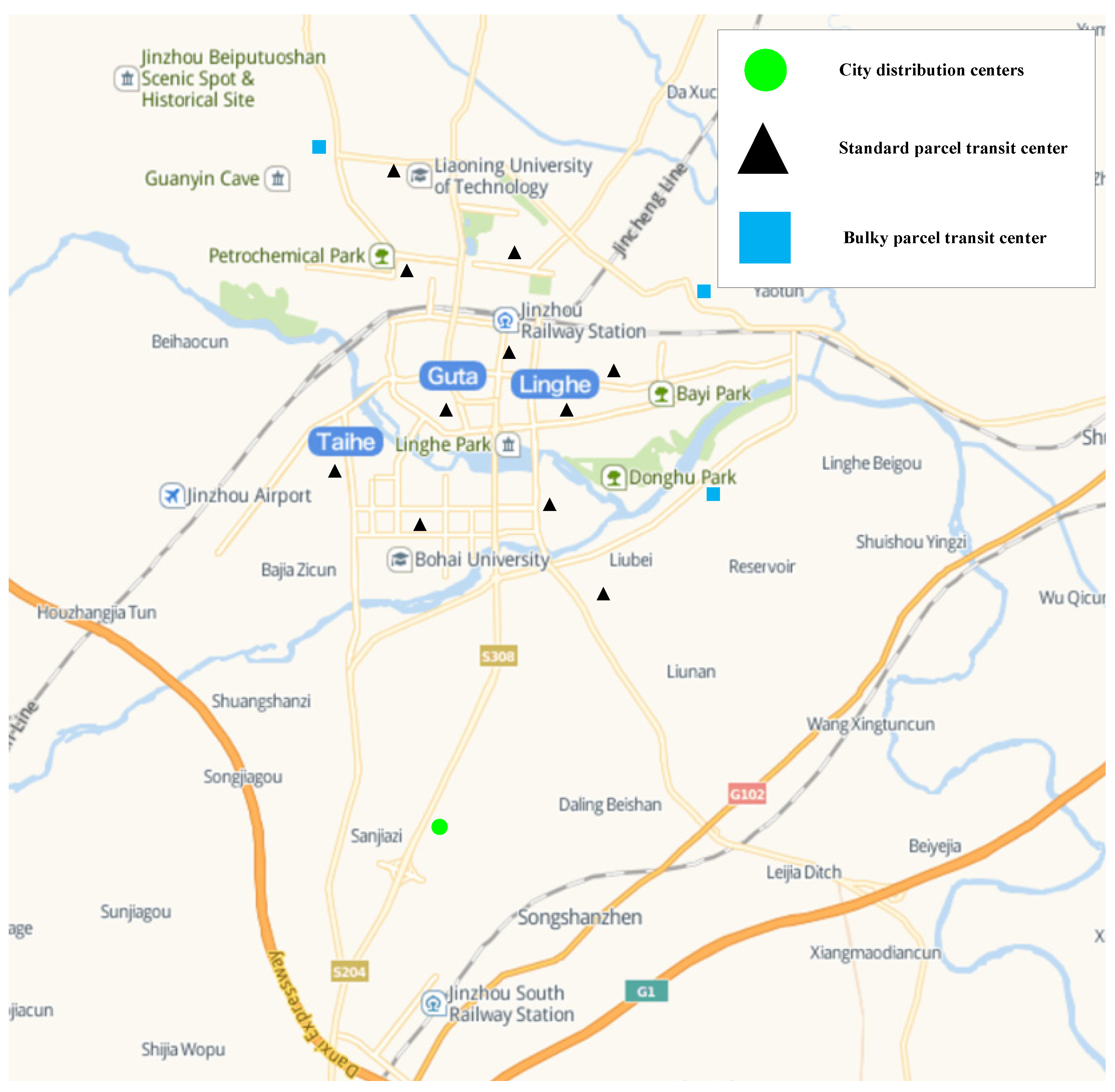
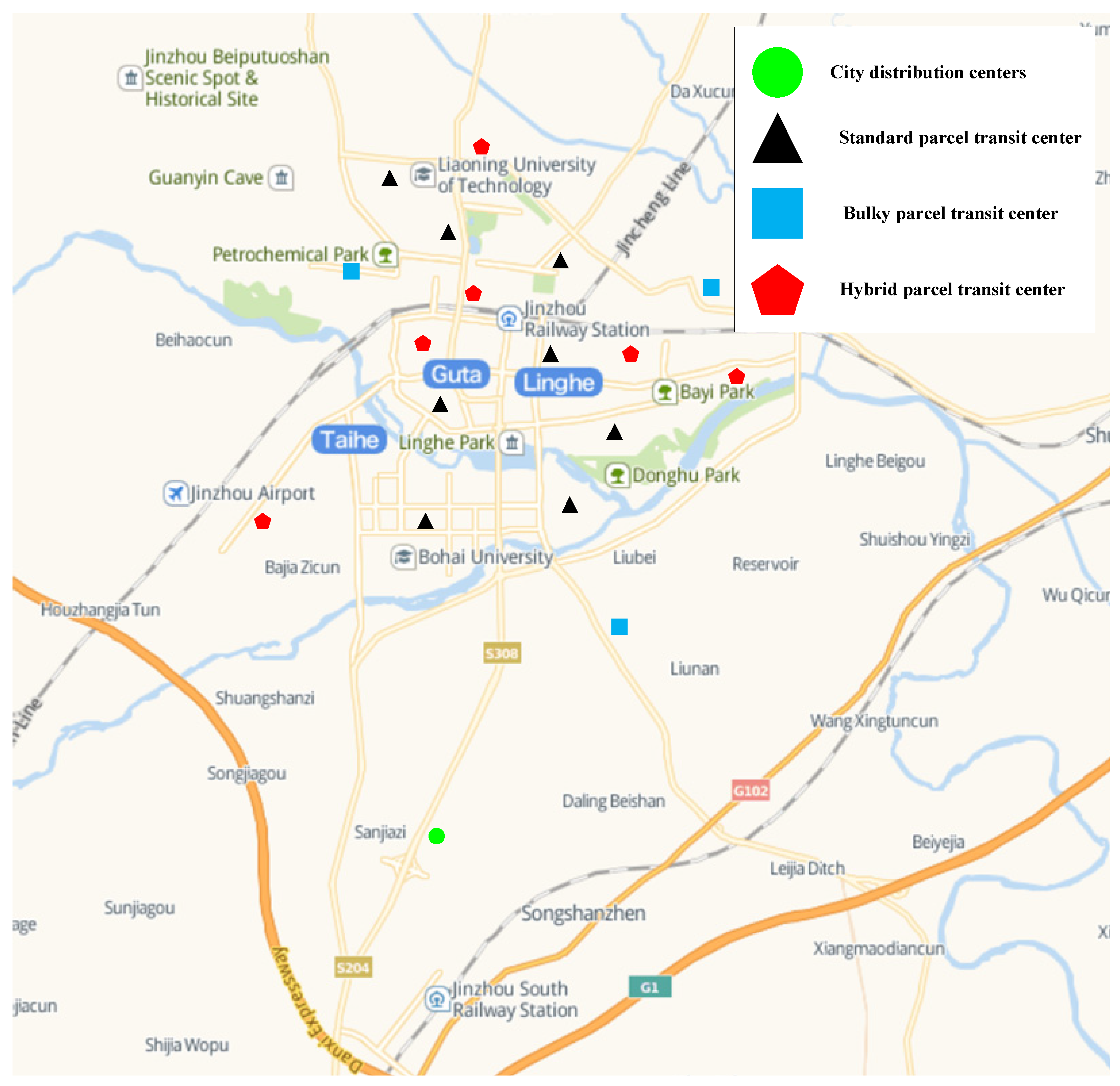
5.2. Example Description and Result Analysis

This paper takes SF Jinzhou Company as an example to analyze the problem of urban logistics site selection-path optimization. SF Jinzhou’s urban logistics network is divided into urban distribution center, SF Express sales department, and terminal demand point, and SF Express business department is equivalent to the urban transit center in this model. The sales department has 3–15 delivery staff; the delivery staff fixed the distribution zone, and the distribution zone covers several terminal demand points. Terminal demand points include types such as delivery points, smart self-pickup lockers, and local merchant cooperation points. SF Jinzhou currently has 336 terminal demand points in the main urban area, including 11 standard parcel transit centers, 3 bulky parcel transit centers, and 1 city distribution center, of which the urban distribution center is responsible for air and land transportation, respectively. Figure 8 shows the distribution of existing transit centers of SF Jinzhou Company.

In daily life, schools and residential areas are mainly standard parcels, while factories, industrial parks, and business districts are mainly large parcels. SF Jinzhou’s models include vans, trucks, electric tricycles, and two-wheelers. The distribution of terminal demand points is highly dense and the distribution frequency is high, and logistics models with small capacity and strong mobility are mostly adopted. Five-ton trucks are used from the urban distribution center to each transit center, electric tricycles are used for standard parcels from the transit center to the terminal demand point, and vans are used for large parcels. According to SF Jinzhou Company’s existing transit center and potential optional points, 76 transfer center candidate points are generated, and the delivery and collection of parcels at 336 terminal demand points are collected. The distance between nodes is obtained through Datamap, and the relevant parameter settings are shown in

Table 6. Parameter setting of SF Jinzhou Company.

Fixed Cost (RMB)			${{\mathit{N}}_{\mathit{p}}}_{\left(\mathbf{Number}\right)}$		Unit Transportation Cost (RMB/km)
${\mathit{f}}_{\mathit{S}}$	${\mathit{f}}_{\mathit{L}}$	${\mathit{f}}_{\mathit{M}\mathit{I}\mathit{X}}$	Standard Package	Bulky Packages	${\mathit{v}}_1$	${\mathit{v}}_2$	${\mathit{v}}_3$
300	800	1000	1500	800	10	2	5

.

According to the data in the above table, this article uses the Python 3.7.3 programming language to implement the above optimization algorithm, and the running platform is Intel Core i7-6700HQ CPU @ 2.60 GHz, Win10 PC. Based on the IHBA proposed in this paper, the three transit center opening schemes under each threshold and the cost are obtained (see

Table 7. Result of optimization under collaborative delivery.

Threshold (kg)	Transit Center (Piece)			Cost (RMB)
	Standard Type	Large Type	Hybrid Type	Fixed Cost	Shipping Cost	Total Cost	Average Unit Price
2	0	17	0	13,600	35,872.87	49,472.87	4.73
5	1	12	2	11,900	31,498.21	43,398.21	4.98
10	4	6	5	11,000	27,981.89	38,981.89	3.73
15	8	3	6	10,800	23,268.98	34,068.98	2.54
20	33	0	1	10,900	29,763.73	40,663.73	3.12
30	46	0	0	13,800	32,873.81	46,673.81	5.98

).

The Figure 9 shows the layout of SF Jinzhou Company’s optimized transit center. The threshold value of the optimization scheme is 15 kg, which is different from the existing threshold of 20 kg with SF Jinzhou Company. A total of 17 transit centers were opened under the optimization plan, including 6 hybrid type, 8 standard type, and 3 large type. The total cost of the optimization scheme is CNY 34,068.98, and the average cost of the parcel list is CNY 2.54. Compared with SF Express’ existing urban logistics network, the total logistics cost and the average unit cost are reduced 9.6%.

6. Conclusions

This paper studies the joint optimization of the threshold setting of large parcels, the location selection of multi-functional transit centers, and the allocation of terminal demand points under the implementation of multi-product (parcel) collaborative distribution by urban logistics enterprises. In the second part of this paper, the threshold setting of large parcels and standard parcels is introduced, and the differences in handling, sorting, and other processing links and related facilities and site configurations between oversized parcels and standard parcels are comprehensively considered, and the type variables of multi-functional transit centers are constructed in the second part of this paper. An integer programming model is constructed with the goal of minimizing the total cost of the logistics system. Firstly, in view of the shortcomings of the original honey badger algorithm, Chebyshev chaotic mapping is first introduced in the initial population processing stage, which effectively maintains the diversity of the population and avoids premature convergence of the algorithm. Then, the refractive mirror learning strategy (RML) is introduced in the foal position update formula to increase the diversity of the population to find better candidate solutions. Finally, the position update of honey badger is carried out by using the strategy of mixing moth fire fighting and golden sinusoid, which fundamentally changes the mining and search mechanism of the honey badger algorithm, so that the search space of the honey badger in the exploration stage is reduced, thereby greatly shortening the optimization time of the honey badger. Through comparative experiments, it is proved that the improved honey badger algorithm has good global and local optimization ability, but also has good robustness. Then, the logistics model established in the second part above was optimized, and the hybrid transit center was opened in a timely manner according to the solution of the lower and upper bound solutions. Finally, the effectiveness of the improved honey badger algorithm is verified by comparing with the CPLEX operation results. Then, according to the operation data of SF Jinzhou, a typical domestic express delivery company, the optimization results of the large parcel threshold, the location layout of the multi-functional transit center, and the allocation of terminal demand points were obtained, and the impact of the distribution mode, the volume of parcels delivered and received, and the service time were analyzed.

From the above many experiments, it is not difficult to see that, on the one hand, the group intelligence algorithm has advantages in solving the problem of logistics site selection and path optimization. On the other hand, from the comparison results of the examples, it can also be obtained that SF Jinzhou Company’s optimized large size threshold is 15 kg, which is different from the existing threshold of 20 kg, and the total cost of the optimization plan is compared with the existing situation, and the total logistics cost and average unit price cost are reduced by 9.6%. Therefore, the optimization scheme presented by the model and algorithm in this paper is robust, which can not only meet the needs of urban logistics enterprises of different parcel scales, but also apply to the daily fluctuation of parcel delivery and collection volume of logistics enterprises of the same type of city. For urban logistics enterprises that operate multiple types of parcels, there is no fixed standard for the selection of large item threshold; urban logistics enterprises need to reasonably select the large size threshold according to the distribution of parcel delivery and collection structure, and comprehensively consider relevant factors. The interval time of parcel distribution will not affect the setting of the threshold, and there is no obvious impact on the average fixed cost and processing cost of parcels, but the average transportation cost will decrease significantly with the increase of the distribution interval time, that is, the main reason for the decrease in total logistics cost is from the reduction of transportation costs.

Based on the experimental research conclusions of this paper and the current development status of large-scale business in the logistics field, this paper puts forward the following suggestions: First, express delivery companies entering the large-scale field should reasonably choose the threshold according to their own conditions. The selection of thresholds is related to the scale and structure of parcel delivery and collection. The second is to reasonably determine the service timeliness; the higher the service timeliness, the higher the frequency of distribution. The high frequency of distribution reduces the delivery and collection volume of parcels in a single batch, which cannot give full play to economies of scale, reduces the utilization rate of logistics resources such as facilities in transit centers, has a low vehicle loading rate, and has a high average cost of a single parcel. In reality, it is necessary to clarify the customer’s timeliness needs, integrate logistics costs and service experience, and reasonably determine the service timeliness. Third, for express delivery companies entering the field of large-scale logistics, in the early stage of the growth of large-scale parcels, they can respond to the increase in demand by increasing the capacity of large-scale vehicles, but when the demand increases to a certain amount, it is also necessary to add corresponding transit centers. Fourth, the operation organization of collaborative distribution is more difficult than that of independent distribution, and the requirements for enterprise management level and information systems are higher. In addition, the delivery time of different types of parcels will also affect the cost of coordinated delivery. Therefore, when other urban logistics enterprises other than SF logistics enterprises implement multi-parcel distribution, they need to conduct a comprehensive assessment according to their own needs and conditions.

References

1. Özmen, M.; Aydoğan, E.K. Robust multi-criteria decision making methodology for real life logistics center location problem. Artif. Intell. Rev. Int. Sci. Eng. J. 2020, 53, 725–751. [Google Scholar] [CrossRef]
2. Zhang, J.; Weng, Z.; Guo, Y. Distribution Center Location Model Based on Gauss-Kruger Projection and Gravity Method. J. Phys. Conf. Ser. 2021, 1972, 012075. [Google Scholar] [CrossRef]
3. Cai, C.; Luo, Y.; Cui, Y.; Chen, F. Solving Multiple Distribution Center Location Allocation Problem Using K-Means Algorithm and Center of Gravity Method Take Jinjiang District of Chengdu as an example. IOP Conf. Ser. Earth Environ. Sci. 2020, 587, 012120. [Google Scholar] [CrossRef]
4. Li, J.; Lei, H.; Wang, G.G. Solving Logistics Distribution Center Location with Improved Cuckoo Search Algorithm. Int. J. Comput. Intell. Syst. 2020, 14, 2. [Google Scholar] [CrossRef]
5. Mei, Z.; Chi, X.; Chi, R. Research on Logistics Distribution Center Location Based on Hybrid Beetle Antennae Search and Rain Algorithm. Biomimetics 2022, 7, 194. [Google Scholar] [CrossRef] [PubMed]
6. Chi, R.; Su, Y.; Qu, Z.; Chi, X. A Hybridization of Cuckoo Search and Differential Evolution for the Logistics Distribution Center Location Problem. Math. Probl. Eng. 2019, 2019, 7051248. [Google Scholar] [CrossRef]
7. Zhang, H.; Shi, Y.; Zhang, X. Optimization for Logistics Center Location in Coastal Tourist Attraction Based on Grey Wolf Optimizer. J. Coast. Res. 2019, 94, 823–827. [Google Scholar] [CrossRef]
8. Yang, L.; Song, X. High-Performance Computing Analysis and Location Selection of Logistics Distribution Center Space Based on Whale Optimization Algorithm. Comput. Intell. Neurosci. 2022, 2022, 2055241. [Google Scholar] [CrossRef]
9. Liu, D.; Hu, X.; Jiang, Q. Design and optimization of logistics distribution route based on improved ant colony algorithm. Optik 2023, 273, 170405. [Google Scholar] [CrossRef]
10. Zhang, S.; Zheng, Y.; Li, G. Research on distribution center layout optimization based on genetic algorithm. J. Phys. Conf. Ser. 2021, 1976, 012010. [Google Scholar] [CrossRef]
11. Wei, Y.; Zhou, L. Soft Time Windows Associated Vehicles Routing Problems of Logistics Distribution Center Using Genetic Simulated Annealing Algorithm. J. Comput. Inf. Technol. 2014, 22, 31–39. [Google Scholar] [CrossRef]
12. Wu, X. Design of logistics distribution center location method based on particle swarm optimization. Acad. J. Eng. Technol. Sci. 2023, 6. [Google Scholar] [CrossRef]
13. Hua, X.; Hu, X.; Yuan, W. Research optimization on logistics distribution center location based on adaptive particle swarm algorithm. Optik 2016, 127, 8443–8450. [Google Scholar] [CrossRef]
14. Liu, X.L.; Zhang, W.Y. Application of Composite Ant Colony Optimization in Logistics Distribution Center Location. Appl. Mech. Mater. 2012, 253, 1476–1481. [Google Scholar] [CrossRef]
15. Li, Y.G. An Improved Bat Algorithm and its Application in the Logistics Distribution Center Location Problem. Appl. Mech. Mater. 2013, 404, 738–743. [Google Scholar] [CrossRef]
16. Shihab, I.F.; Oishi, M.M.; Islam, S.; Banik, K.; Arif, H. A Machine Learning Approach to Suggest Ideal Geographical Location for New Restaurant Establishment. In Proceedings of the 2018 IEEE 6th Region 10 Humanitarian Technology Conference (R10-HTC), Malambe, Sri Lanka, 6–8 December 2018. [Google Scholar]
17. Dai, X.; Chen, M.; Zhou, Y. Optimal logistics transportation and route planning based on fpga processor real-time system and machine learning. Microprocess. Microsyst. 2021, 80, 103621. [Google Scholar] [CrossRef]
18. Song, F.; Lu, X.; Li, K. Research on Location Model of Shanghai Express Outlets Based on Big Data and Machine Learning. In Proceedings of the 8th International Symposium on Project Management, China (ISPM2020), Beijing, China, 4 July 2020; pp. 1430–1436. [Google Scholar] [CrossRef]
19. Mirjalili, S. Moth-flame optimization algorithm: A novel nature-inspired heuristic paradigm. Knowl. Based Syst. 2015, 89, 228–249. [Google Scholar] [CrossRef]
20. Arora, S.; Singh, S. Butterfly optimization algorithm: A novel approach for global optimization. Soft Comput. 2019, 23, 715–734. [Google Scholar] [CrossRef]
21. Mirjalili, S. SCA: A Sine Cosine Algorithm for solving optimization problems. Knowl.-Based Syst. 2016, 96, 120–133. [Google Scholar] [CrossRef]
22. Trojovský, P.; Dehghani, M. Pelican Optimization Algorithm: A Novel Nature-Inspired Algorithm for Engineering Applications. Sensors 2022, 22, 855. [Google Scholar] [CrossRef]
23. Zervoudakis, K.; Tsafarakis, S. A mayfly optimization algorithm. Comput. Ind. Eng. 2020, 145, 106559. [Google Scholar] [CrossRef]
24. Tanyildizi, E.; Demir, G. Golden Sine Algorithm: A Novel Math-Inspired Algorithm. Adv. Electr. Comput. Eng. 2017, 17, 71–78. [Google Scholar] [CrossRef]
25. Askarzadeh, A. A novel metaheuristic method for solving constrained engineering optimization problems: Crow search algorithm. Comput. Struct. 2016, 169, 1–12. [Google Scholar] [CrossRef]
26. Meraihi, Y.; Gabis, A.B.; Mirjalili, S.; Ramdane-Cherif, A. Grasshopper Optimization Algorithm: Theory, Variants, and Applications. IEEE Access 2021, 9, 50001–50024. [Google Scholar] [CrossRef]
27. Mirjalili, S. The Ant Lion Optimizer. Adv. Eng. Softw. 2015, 83, 80–98. [Google Scholar] [CrossRef]
28. Alomari, A.; Phillips, W.; Aslam, N.; Comeau, F. Swarm Intelligence Optimization Techniques for Obstacle-Avoidance Mobility-Assisted Localization in Wireless Sensor Networks. IEEE Access 2017, 6, 22368–22385. [Google Scholar] [CrossRef]
29. Szczepański, E.; Jachimowski, R.; Izdebski, M.; Jacyna-Gołda, I. Warehouse location problem in supply chain designing: A simulation analysis. Arch. Transp. 2019, 50, 101–110. [Google Scholar] [CrossRef]
30. Pyza, D.; Jacyna-Gołda, I.; Gołda, P. Problems of Deliveries in Urban Agglomeration Distribution Systems. In Directions of Development of Transport Networks and Traffic Engineering; Macioszek, E., Sierpiński, G., Eds.; Lecture Notes in Networks and Systems; Springer: Cham, Switzerland, 2018; Volume 51, pp. 174–183. [Google Scholar] [CrossRef]
31. Hashim, F.A.; Houssein, E.H.; Hussain, K.; Mabrouk, M.S.; Al-Atabany, W. Honey Badger Algorithm: New metaheuristic algorithm for solving optimization problems. Math. Comput. Simul. 2021, 192, 84–110. [Google Scholar] [CrossRef]
32. Long, W.; Wu, T.; Jiao, J.; Tang, M.; Xu, M. Refraction-learning-based whale optimization algorithm for high-dimensional problems and parameter estimation of PV model. Eng. Appl. Artif. Intell. 2020, 89, 103457. [Google Scholar] [CrossRef]
33. Dunia, S.; Ali, R. Chaotic Sine-Cosine Optimization Algorithms. Int. J. Soft Comput. 2018, 13, 108–122. [Google Scholar]
34. Wu, H.; Wu, P.; Xu, K.; Li, F. Finite element model updating using crow search algorithm with Levy flight. Int. J. Numer. Methods Eng. 2020, 121, 2916–2928. [Google Scholar] [CrossRef]
35. Sankaranarayanan, S.; Swaminathan, G.; Sivakumaran, N.; Radhakrishnan, T.K. A novel hybridized grey wolf optimzation for a cost optimal design of water distribution network. In Proceedings of the 2017 Computing Conference, London, UK, 18–20 July 2017. [Google Scholar]
36. Chen, S. Chaotic particle swarm optimization fusion FCM clustering algorithm based on chebyshev mapping. Comput. Appl. Softw. 2015, 32, 255–258. [Google Scholar]
37. Zhang, Y.; Wang, P.; Yang, H.; Cui, Q. Optimal dispatching of microgrid based on improved moth-flame optimization algorithm based on sine mapping and Gaussian mutation. Syst. Sci. Control Eng. 2022, 10, 115–125. [Google Scholar] [CrossRef]
38. Yuan, P.; Zhang, T.; Yao, L.; Lu, Y.; Zhuang, W. A Hybrid Golden Jackal Optimization and Golden Sine Algorithm with Dynamic Lens-Imaging Learning for Global Optimization Problems. Appl. Sci. 2022, 12, 9709. [Google Scholar] [CrossRef]
39. Li, J.; Le, M. Improved whale optimization algorithm based on image selection. Trans. Nanjing Univ. Aeronaut. Astronaut. 2020, 37, 115–123. [Google Scholar]
40. Deb, K.; Deb, D. Analysing mutation schemes for realparameter genetic algorithms. Int. J. Artif. Intell. Soft Comput. 2014, 4, 1–28. [Google Scholar]
41. Deb, K.; Mohan, M.; Mishra, S. Evaluating the ε-Domination Based Multi-Objective Evolutionary Algorithm for a Quick Com-putation of Pareto-Optimal Solutions. Evol. Comput. 2005, 13, 501–525. [Google Scholar] [CrossRef]
42. Perolat, J.; Couso, I.; Loquin, K.; Strauss, O. Generalizing the Wilcoxon rank-sum test for interval data. Int. J. Approx. Reason. 2015, 56, 108–121. [Google Scholar] [CrossRef]
43. Derrac, J.; García, S.; Molina, D.; Herrera, F. A practical tutorial on the use of nonparametric statistical tests as a methodology for comparing evolutionary and swarm intelligence algorithms. Swarm Evol. Comput. 2011, 1, 3–18. [Google Scholar] [CrossRef]
Figure 1. Urban logistics network under the coordinated distribution for standard and large items.
Applsci 13 06805 g001
Figure 2. Smell intensity of honey badger.
Applsci 13 06805 g002
Figure 3. The mining phase.
Applsci 13 06805 g003
Figure 4. The original trajectory of the honey badger and the trajectory after adding the golden sine.
Applsci 13 06805 g004
Figure 5. Refraction mirror learning diagram.
Applsci 13 06805 g005
Figure 6. Solution approach of the IHBA.
Applsci 13 06805 g006
Figure 7. Average convergence curves of different algorithms. (a) is the average convergence curve of the test function F1; (b) is the average convergence curve of the test function F2; (c) is the average convergence curve of the test function F3; (d) is the average convergence curve of the test function F4; (e) is the average convergence curve of the test function F5; (f) is the average convergence curve of the test function F6; (g) is the average convergence curve of the test function F7; (h) is the average convergence curve of the test function F8; (i) is the average convergence curve of the test function F9; (j) is the average convergence curve of the test function F10; (k) is the average convergence curve of the test function F11.
Applsci 13 06805 g007aApplsci 13 06805 g007bApplsci 13 06805 g007cApplsci 13 06805 g007d
Figure 8. Current transfer center distribution of SF Jinzhou Company.
Applsci 13 06805 g008
Figure 9. Optimized transfer center distribution of SF Jinzhou Company.
Applsci 13 06805 g009