Article

Prediction of Chatter Stability in Bull-Nose End Milling of Thin-Walled Cylindrical Parts Using Layered Cutting Force Coefficients

1
School of Mechanical and Materials Engineering, North China University of Technology, Beijing 100144, China
2
Key Laboratory of High Performance Manufacturing for Aero Engine, Ministry of Industry and Information Technology, Northwestern Polytechnical University, Xi’an 710072, China
*
Authors to whom correspondence should be addressed.
Appl. Sci. 2023, 13(11), 6737; https://doi.org/10.3390/app13116737
Submission received: 18 April 2023 / Revised: 24 May 2023 / Accepted: 30 May 2023 / Published: 1 June 2023
(This article belongs to the Section Mechanical Engineering)

Abstract

:
During the bull-nose end milling operations of thin-walled structures, chatter usually occurs and adversely affects cutter performance, finished surface quality, and production efficiency. To accurately predict chatter stability, a suitable dynamic model with effective system parameters is required. In this article, a three-degree-of-freedom (3-DOF) dynamic model is developed to analyze the milling stability of the thin-walled cylinders, in which the dynamics of the bull-nose end mill along the x-axis and y-axis directions and the dynamic of the workpiece along the z-axis direction are taken into account. Then, the cutter-workpiece engagement (CWE) is extracted by employing a slice-intersection-based approach. And the layered cutting force coefficients are identified by considering the influences of varying cutter diameters on the cutting speed. Thereafter, the semi-discretization method (SDM) is adopted to compute the stability lobe diagram (SLD). In the end, a group of milling tests are carried out on a thin-walled cylinder to validate the accuracy and reliability of the proposed model, and the results show that the model predictions agree well with the experimental data.

1. Introduction

Thin-walled structures are commonly applied in the aerospace, marine, and automotive industries owing to their incomparable advantages, such as lightweight and high specific strength. Considering the high material removal rate and sleek finished surface, bull-nose end milling has become a popular operation for the manufacturing of thin-walled parts, such as aero-engine blades, impellers, and casings [1,2,3]. These parts have complex and thin-walled structures and often bring many machining difficulties and challenges. Chatter is essentially a self-excited vibration and usually appears in the milling process. It not only pulls down the material removal rate but also results in a coarse finished surface, premature tool wear, excessive cutting noise, and so on [4,5]. Chatter has long been one of the main problems during the milling operation. Thus, to avoid chatter, the milling operation must be performed in a steady state [6]. Furthermore, the calculation of SLD has become and still is an important research topic in high-quality machining.
Presently, two primary mathematical solutions are employed to construct the SLD, namely the analytical and numerical approaches. In terms of the analytical approaches, Altintas and Budak [7] proposed a single-frequency solution (SFS) on the basis of the truncated Fourier series of the cyclical cutting forces. The SFS is also known as the zeroth-order approximation (ZOA) approach, which can plot the SLD efficiently. However, it fails to compute the extra stability boundaries and the doubling bifurcations. For solving this question, Budak and Altintas [8,9] subsequently reported a multi-frequency solution (MFS), where the higher-order parts of the Fourier series are adopted. Merdol and Altintas [10] expanded the application of the MFS to machining conditions with small radial depths of cut. The disadvantage of the MFS is that it consumes more computing time. In comparison with the analytical approaches, more investigations have concentrated on numerical approaches [11]. Insperger and Stépán [12] reported an important SDM to evaluate milling stability. In this approach, the zeroth-order piecewise constant function is employed to approach the delayed part. To achieve better solution accuracy and quicker convergence rates, many high-order SDMs were developed. Insperger et al. [13] took into account the first-order approximation of the delayed term (namely the first SDM). Jiang et al. [14] investigated the second-order approximation of the delayed term (namely the second SDM). Yan et al. [15] suggested a third SDM and a fourth SDM. On the other hand, Ding et al. [16] pioneered the influential full-discretization method (FDM), which has a higher computational efficiency. In the FDM, in addition to the delayed term, the state term is also approximated by employing linear interpolation. Subsequently, many other approaches inspired by the FDM have been proposed, just like the 2nd FDM [17], the 3rd FDM [18], the updated FDM (UFDM) [19], the 2nd UFDM [20], and the 3rd UFDM [21].
During the bull-nose end finishing process of thin-walled or thin-floor parts, the influence of the workpiece dynamics cannot be neglected [22,23,24]. Campa et al. [25,26] modeled the dynamics of the thin-floor structure as a 1-DOF system and predicted the SLD in bull-nose end finish milling. Based on this study, the influence of the material removal on the bull-nose end milling stability is analyzed, and the three-dimensional (3D) SLD along the toolpath is calculated [27]. Later, a half-active magnetorheological damper is designed to dampen regenerative chatter for the bull-nose end finishing of thin floors [28]. Zhou et al. [29] simplified the dynamics of the aero-engine casings into a 1-DOF model along the workpiece’s radial direction. The model only takes into account the workpiece flexibility and is able to evaluate the SLD for different small lead angles. The above models only consider the dynamics of the workpiece, while the cutter is assumed to have a rigid body. It is essential to establish a multi-DOF milling system when neither the tool nor the workpiece dynamics can be ignored [30,31,32]. However, the 3-DOF stability prediction model for bull-nose end milling has been rarely explored. Especially for the cylindrical part, which has a ring-shaped and closed geometry structure. Yan et al. [33] modeled a 3-DOF milling system by taking into account the tool dynamics along the x and y directions and the workpiece dynamics along the z direction. Dang et al. [34] suggested a 3-DOF milling stability model for thin-floor components, in which the static and dynamic deflections of the tool and the workpiece are considered together.
In the chatter stability model, the cutting force coefficients are very important for the calculation of SLD [3,35]. Currently, most models ignore the effect of the cutter diameter variation and treat the cutting force coefficients as constants for the bull-nose or ball end milling [36], which can result in inaccurate stability predictions. Based on previous research [29], this article presents a 3-DOF chatter stability model that takes into account the effects of cutter diameter variation on the cutting speed. In Section 2, the 3-DOF milling system for the bull-nose end milling of a thin-walled cylinder is established. The dynamic cutting force model, CWE calculation, identification of layered cutting force coefficients, and SLD calculation with SDM are also conducted in this section. In Section 3, a group of milling tests are performed to validate the accuracy and reliability of the 3-DOF chatter stability model. Finally, some conclusions are proposed.

2. 3-DOF Chatter Stability Model

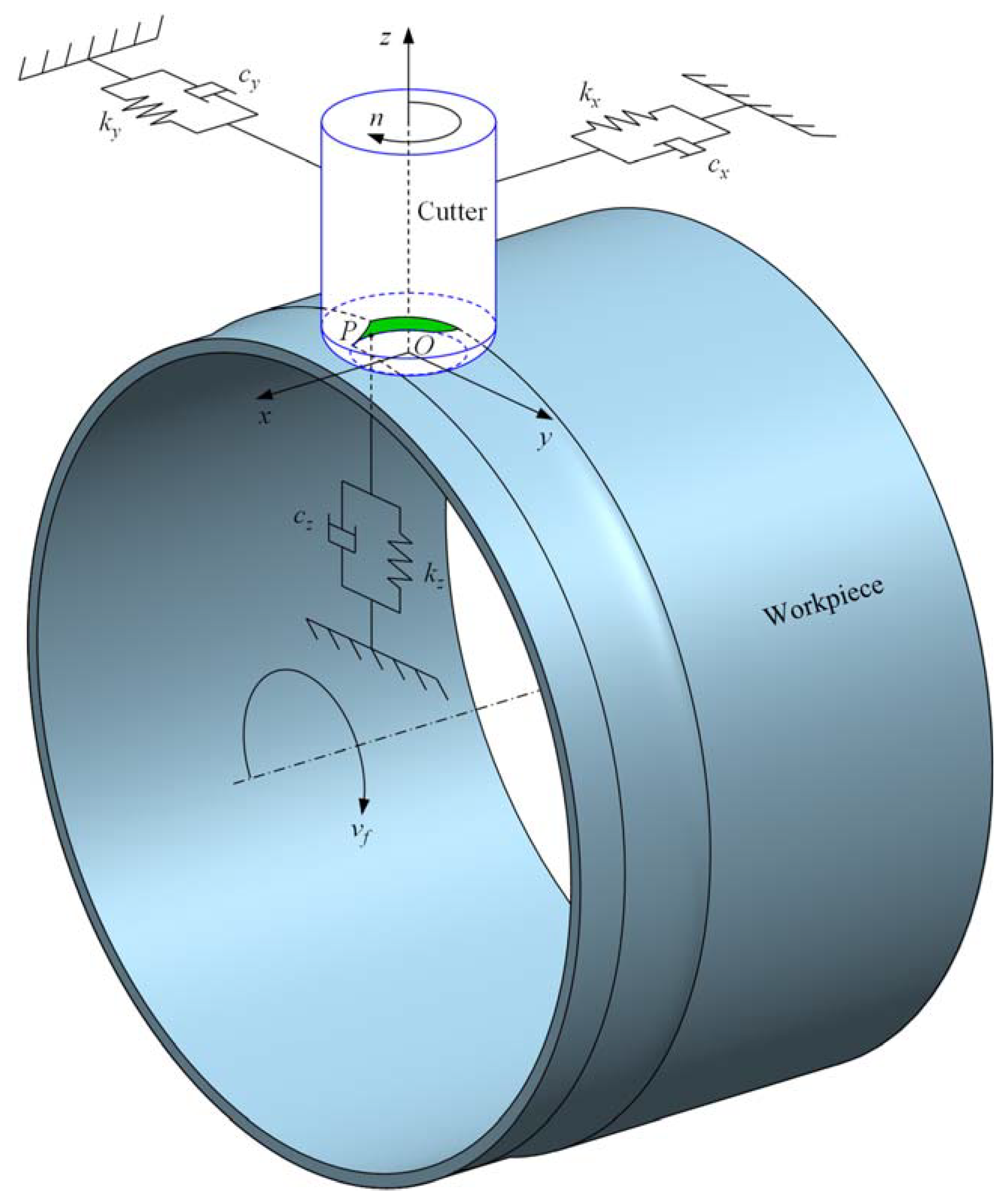
2.1. Milling System for a Thin-Walled Cylinder

During the bull-nose end milling process of thin-walled cylinders, both the cutter and workpiece are regarded as flexible. The dynamic milling system for a thin-walled cylinder is demonstrated in Figure 1, which can be delineated by a 3-DOF mass-spring-damper model. In the x-axis and y-axis directions, a 2-DOF dynamic model is employed to delineate the cutter, while an absolutely rigid body is applied to assume the workpiece. In the z-axis direction, a 1-DOF dynamic model is employed to delineate the workpiece, while an absolutely rigid body is applied to assume the cutter. O-xyz stands for the cutter coordinate system (CCS). The origin O is centered at the end of the cutter. The workpiece feed direction is specified as the y-axis. The cutter axis direction is specified as the z-axis. The right-hand rule is employed to identify the x-axis. Based on the previous study [29], the cutting contact point P is identified according to the eccentric amount from the cutter axis to the centerline of the workpiece.
The dynamic equation of the 3-DOF bull-nose end milling system is established as follows:
m x 0 0 0 m y 0 0 0 m z x ¨ c ( t ) y ¨ c ( t ) z ¨ w ( t ) + c x 0 0 0 c y 0 0 0 c z x ˙ c ( t ) y ˙ c ( t ) z ˙ w ( t ) + k x 0 0 0 k y 0 0 0 k z x c ( t ) y c ( t ) z w ( t ) = F x F y F z
where mx, cx, and kx denote the modal mass, damping, and stiffness of the cutter, respectively, along the x-axis direction. my, cy, and ky denote the modal mass, damping, and stiffness of the cutter, respectively, along the y-axis direction. mz, cz, and kz denote the modal mass, damping, and stiffness of the workpiece, respectively, along the z-axis direction. xc(t) and yc(t) denote the cutter displacements along the x-axis and y-axis directions, respectively. zw(t) denotes the workpiece displacement along the z-axis direction. Fx, Fy, and Fz denote the cutting forces along the x-axis, y-axis, and z-axis directions, respectively.

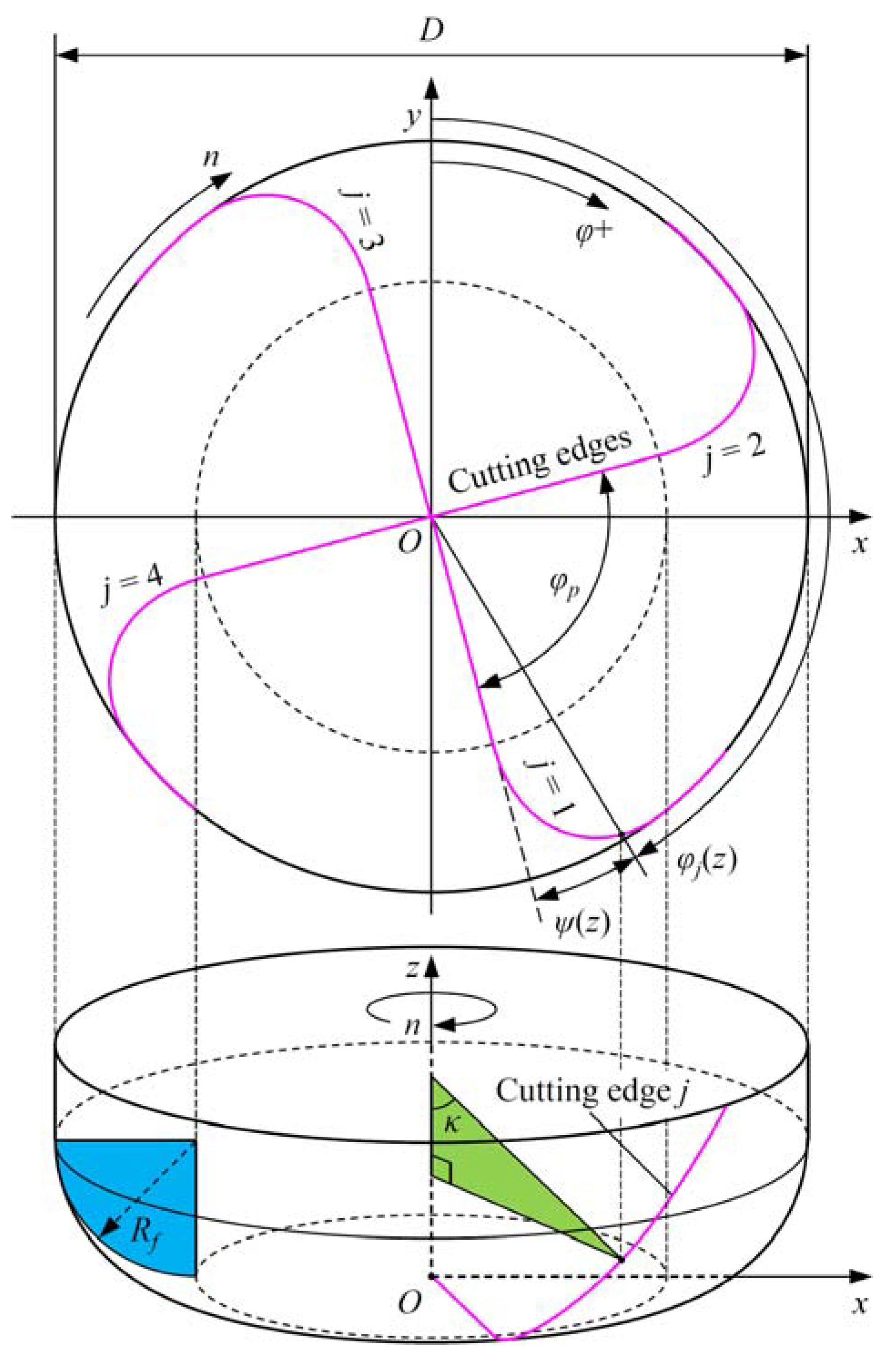
2.2. Dynamic Cutting Force Modeling for Bull-Nose End Milling

Figure 2 demonstrates a bull-nose end cutter, which is characterized by two main parameters: the fillet radius Rf and the cutter diameter D.
For the bull-nose end milling process, the chip thickness can be distributed between the static and dynamic components. The static component is disregarded because it has no influence on milling stability [37]. The dynamic component of cutting-edge j is determined as follows:
h d ( φ j , κ ) = sin φ j sin κ cos φ j sin κ cos κ Δ x Δ y Δ z
where
φ j ( z ) = φ + ( j 1 ) φ p ψ ( z ) = 2 π n 60 t + ( j 1 ) 2 π N 2 z tan β D
κ ( z ) = arccos R f z R f , ( z < R f )
Δ x Δ y Δ z = x c ( t ) x c ( t T ) y c ( t ) y c ( t T ) z w ( t T ) z w ( t )
where φj denotes the radial immersion angle of cutting-edge j. φ denotes the rotation angle of the cutting edge. φp denotes the pitch angle of the cutter. ψ(z) denotes the radial lag angle caused by the local helix angle. n denotes the spindle speed. t denotes the time parameter. N denotes the number of cutting edges. β denotes the constant helix angle of the cutter. κ denotes the axial immersion angle. Δx, Δy, and Δz denote the x-axis, y-axis, and z-axis dynamic displacements in the CCS. xc(t) and yc(t) denote the dynamic displacements of the cutter at the present time t. xc(tT) and yc(tT) denote the dynamic displacements of the cutter at previous tooth periods tT. zw(t) denotes the dynamic displacement of the workpiece at the present time. t. zw(tT) denotes the dynamic displacements of the workpiece at previous tooth periods tT.
The dynamic cutting forces in the CCS can be established as follows:
F x F y F z = j = 1 N l = 1 M g ( φ j ) T ( φ j , κ ) K t , l K r , l K a , l h d ( φ j , κ ) d z sin κ
where
g ( φ j ) = 1 φ s t , l < φ j < φ e x , l 0 otherwise
T ( φ j , κ ) = cos φ j sin φ j sin κ sin φ j cos κ   sin φ j cos φ j sin κ cos φ j cos κ 0 cos κ sin κ
where M denotes the number of axial cutting disk elements. g(φj) denotes a unit step function to decide whether the flute is in or out of the cutting state. φst,l and φex,l denote the start and exit angles of the cutting disk element l, respectively. T(φj, κ) denotes the rotational transformation matrix. Kt,l, Kr,l, and Ka,l denote the layered tangential, radial, and axial cutting force coefficients on the cutting disk element l, respectively.
Equation (6) delineates a linear cutting force model where the dynamic chip thickness is not correlated with the feed rate [38]. It can be converted into the following matrix form:
F x F y F z = H ( t ) Δ x Δ y Δ z = h x x h x y h x z h y x h y y h y z h z x h z y h z z Δ x Δ y Δ z
where
h x x = j = 1 N l = 1 M g ( φ j ) K t , l sin φ j cos φ j sin κ K r , l sin 2 φ j sin 2 κ K a , l sin 2 φ j sin κ cos κ d z sin κ h x y = j = 1 N l = 1 M g ( φ j ) K t , l cos 2 φ j sin κ K r , l sin φ j cos φ j sin 2 κ K a , l sin φ j cos φ j sin κ cos κ d z sin κ h x z = j = 1 N l = 1 M g ( φ j ) K t , l cos φ j cos κ + K r , l sin φ j sin κ cos κ + K a , l sin φ j cos 2 κ d z sin κ h y x = j = 1 N l = 1 M g ( φ j ) K t , l sin 2 φ j sin κ K r , l sin φ j cos φ j sin 2 κ K a , l sin φ j cos φ j sin κ cos κ d z sin κ h y y = j = 1 N l = 1 M g ( φ j ) K t , l sin φ j cos φ j sin κ K r , l cos 2 φ j sin 2 κ K a , l cos 2 φ j sin κ cos κ d z sin κ h y z = j = 1 N l = 1 M g ( φ j ) K t , l sin φ j cos κ + K r , l cos φ j sin κ cos κ + K a , l cos φ j cos 2 κ d z sin κ h z x = j = 1 N l = 1 M g ( φ j ) K r , l sin φ j sin κ cos κ K a , l sin φ j sin 2 κ d z sin κ h z y = j = 1 N l = 1 M g ( φ j ) K r , l cos φ j sin κ cos κ K a , l cos φ j sin 2 κ d z sin κ h z z = j = 1 N l = 1 M g ( φ j ) K r , l cos 2 κ + K a , l sin κ cos κ d z sin κ
where hxx, hxy, hxz, hyx, hyy, hyz, hzx, hzy, and hzz are the matrix coefficients.

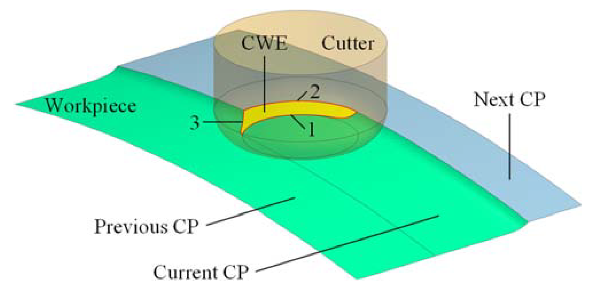
2.3. Calculation of CWE

CWE signifies the instantaneous contact interface while a bull-nose end mill is cutting a thin-walled cylinder. It is one of the foundations for modeling the dynamics of the milling system. During the semi-finish milling or finish milling of thin-walled cylinders, the cutting edges on the toroidal surface of a bull-nose end cutter are applied to end milling, giving rise to a smaller axial depth of cut and a larger machined strip width [39,40].
As shown in Figure 3, the CWE for the bull-nose end milling of thin-walled cylindrical parts consists of three boundaries. Boundary 1 is the cutter profile curve in the current feed direction view. Boundary 2 is the intersection curve between the uncut surface of the workpiece and the toroidal surface of the tool. Boundary 3 is the intersection curve between the workpiece transition surface left by the previous cutting path (CP) and the toroidal surface of the tool. Furthermore, the workpiece transition surface can be generated by a series of boundaries 1, which correspond to each cutting contact point along the previous cutting path. Therefore, the calculation of boundary 1 is the key to determining the CWE at an arbitrary cutting contact point.
As shown in Figure 4, a slice Si can be obtained by offsetting the workpiece’s machined surface Sm outward. Furthermore, the intersection curve Ci between the slice Si and the cutter’s toroidal surface Sc can also be calculated. The boundary points Pi and Qi are determined by employing the closest lines from the two auxiliary planes Pr1 and Pr2 to the intersection curve Ci. The normal directions of the two reference planes Pr1 and Pr2 are simultaneously orthogonal to the workpiece feed direction and the cutter axis direction. The two boundary points are located on boundary 1 and represent the maximum view width of the intersection curve Ci in the workpiece feed direction view. Then, the CWE boundaries can be identified using the intersection curve Ca and a spline obtained by fitting a series of boundary points. The surface trimming tool can be used to extract the engagement geometry for the following cut condition.
The flowchart of the CWE calculation algorithm is shown in Figure 5. And the detailed steps of the CWE calculation algorithm are described in the following:
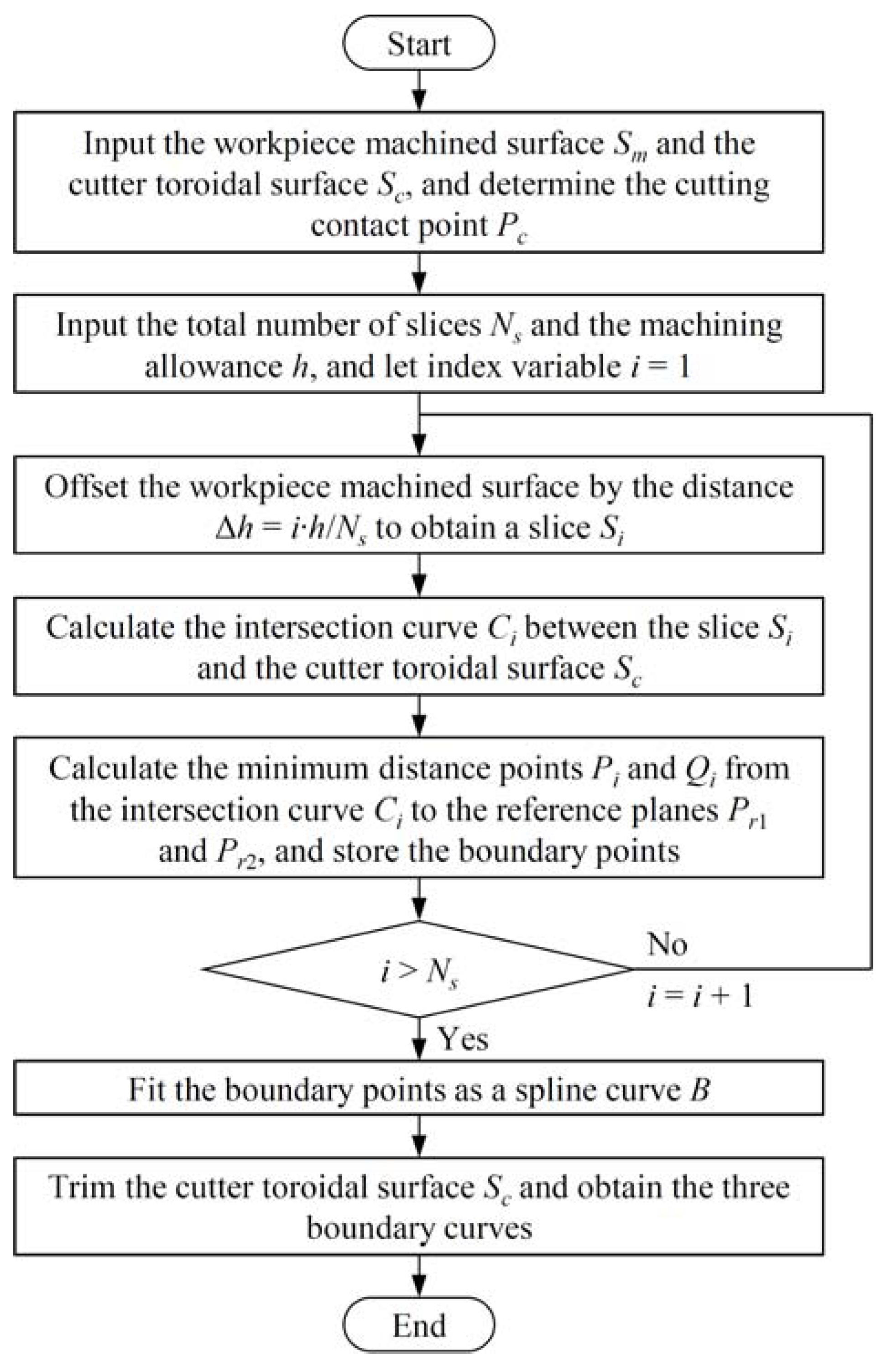
  • Input the machined surface of the workpiece Sm and the toroidal surface of the tool Sc, and determine the cutting contact point Pc according to the cutter axis orientation and the milling line position. The machined surface of the workpiece Sm and the toroidal surface of the tool Sc are tangent to each other at the cutting contact point Pc;
  • Input the total number of slices Ns and the machining allowance h, and set the initial value of an index variable i to 1;
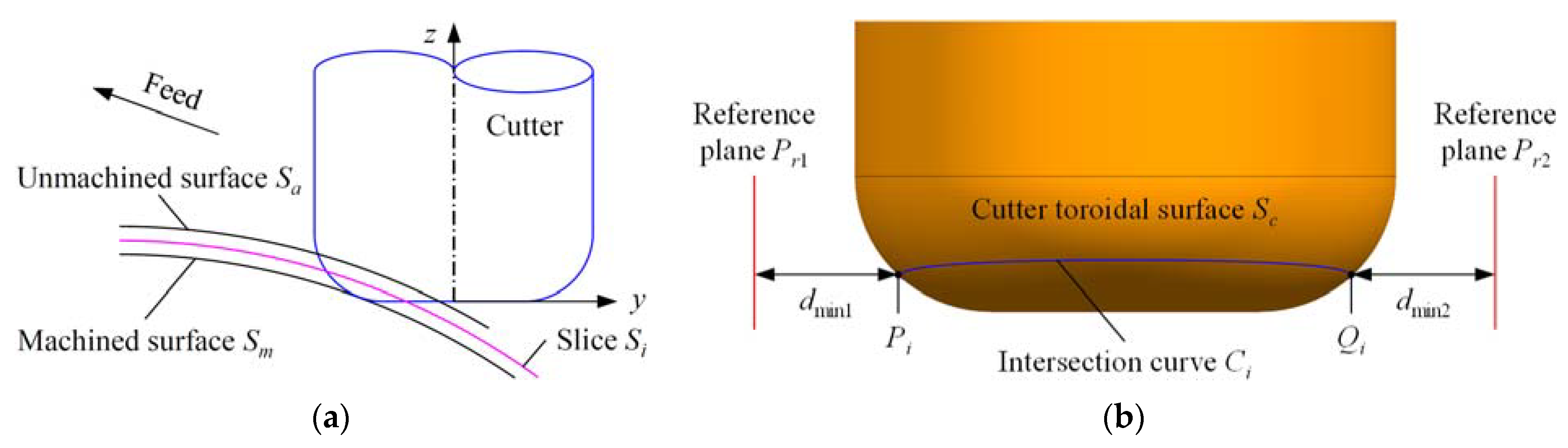
  • Offset the workpiece’s machined surface Sm towards the outside by the distance Δh = i∙h/Ns to obtain a slice Si;
  • Calculate the intersection curve Ci between the slice Si and the toroidal surface of the tool Sc. The intersection curve Ci is essentially boundary 2 with the corresponding machining allowance;
  • Calculate the minimum distance points Pi and Qi from the intersection curve Ci to the reference planes Pr1 and Pr2, and store the minimum distance points into the set of boundary points {P};
  • Go to Step (3) and repeat the process until the index variable i is greater than the total number of slices Ns;
  • Fit the set of boundary points {P} of the CWE as a spline curve B;
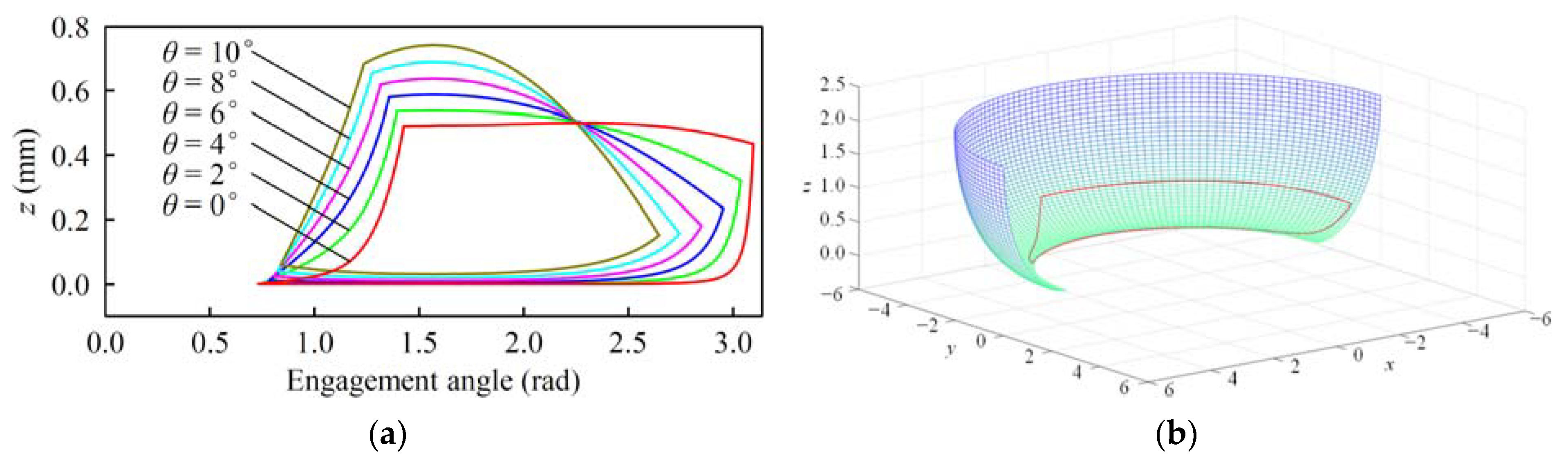
  • Trim the cutter’s toroidal surface Sc using the spline curve B and the intersection curve Ca to extract the CWE in bull-nose end slotting of the thin-walled cylindrical workpiece. The CWEs under the following cut conditions can be obtained by trimming operations.

2.4. Identification of Layered Cutting Force Coefficients

For the toroidal surface of a bull-nose end cutter, the diameter varies continuously along the cutter’s axis direction. The cutting force coefficients are identified by the fact that the measured average cutting forces per tooth are equal to the predicted ones [41,42]. The predicted average cutting forces acting on the lth cutting disk element are given as follows:
F ¯ q , l = 1 φ p φ s t , l φ e x , l z 1 , l z 2 , l d F q , l ( φ , z ) d φ , ( q = x , y , z )
where z1,l and z2,l are the contact boundaries of the lth cutting disk element within the cut.
In the bull-nose end milling experiments, the measured cutting forces are obtained at various axial depths of the cut. The differences in average cutting forces between two adjacent axial depths of cut are calculated so as to acquire the average cutting forces corresponding to each cutting disk element:
F ¯ q , l = F ¯ q ( z l ) F ¯ q ( z l 1 ) , ( q = x , y , z ;   l = 1 , 2 , 3 , , N l )
where zl denotes the lth axial depth of cut and z0 = 0, representing non-cutting. Nl is the number of layers.
The instantaneous cutting forces generated on the lth axial cutting disk element at the radial immersion angle φ are expressed as follows:
F x , l F y , l F z , l = f t 2 A u 1 u 2 u 3
where
A = K t , l sin 2 φ j 2 K r , l sin 2 φ j 2 K a , l sin 2 φ j 2 K t , l sin 2 φ j 2 K r , l sin 2 φ j K a , l sin 2 φ j 0 2 K a , l sin φ j 2 K r , l sin φ j
u 1 = z z 2 , l z 1 , l
u 2 = R f 2 E 1 E 2 + arcsin E z 2 , l z 1 , l
u 3 = 1 R f R f z z 2 2 z 2 , l z 1 , l
E = R f z R f
where ft is the normal feed per tooth.
The instantaneous cutting forces are averaged within the radial immersion interval and expressed as follows:
F ¯ x , l F ¯ y , l F ¯ z , l = f t φ p B K t , l K r , l K a , l
where
B = v 3 u 1 ( v 2 v 1 ) u 2 ( v 2 v 1 ) u 3 ( v 1 v 2 ) u 1 v 3 u 2 v 3 u 3 0 v 4 u 3 v 4 u 2
v 1 = 1 2 φ φ e x , l φ s t , l
v 2 = 1 4 sin ( 2 φ ) φ e x , l φ s t , l
v 3 = 1 4 cos ( 2 φ ) φ e x , l φ s t , l
v 4 = cos φ φ e x , l φ s t , l
Therefore, the cutting force coefficients of the lth axial cutting disk element are determined as follows:
K t , l = 2 π f t N u 1 v 3 F ¯ x , l ( v 2 v 1 ) F ¯ y , l v 3 2 + ( v 2 v 1 ) 2 K r , l = 2 π f t N ( u 2 2 + u 3 2 ) u 2 [ ( v 2 v 1 ) F ¯ x , l + v 3 F ¯ y , l ] v 3 2 + ( v 2 v 1 ) 2 u 3 F ¯ z , l v 4 K a , l = 2 π f t N ( u 2 2 + u 3 2 ) u 3 [ ( v 2 v 1 ) F ¯ x , l + v 3 F ¯ y , l ] v 3 2 + ( v 2 v 1 ) 2 + u 2 F ¯ z , l v 4

2.5. Calculation of SLD with SDM

Equation (1) can be represented by the matrix equation as follows:
M q ¨ ( t ) + C q ˙ ( t ) + K q ( t ) = H ( t ) q ( t ) q ( t T )
where
M = m x 0 0 0 m y 0 0 0 m z
C = c x 0 0 0 c y 0 0 0 c z
K = k x 0 0 0 k y 0 0 0 k z
q ( t ) = x c ( t ) y c ( t ) z w ( t )
where M, C, and K denote the modal mass matrix, the modal damping matrix, and the modal stiffness matrix of the 3-DOF milling system, respectively. q(t) denotes the displacement vector.
At present, the SDM serves as an effective and widely applied method to calculate SLD. According to Insperger and Stépán’s theory [11], Equation (26) is rewritten in the following state-space form:
Q ˙ ( t ) = R ( t ) Q ( t ) + S ( t ) Q ( t τ )
with
R ( t ) = R ( t + T )
S ( t ) = S ( t + T )
where
Q ( t ) = q ( t ) q ˙ ( t )
R ( t ) = 0 I M 1 K M 1 H ( t ) M 1 C
S ( t ) = 0 0 M 1 H ( t ) 0
where Q(t) denotes the time-state vector. R(t) and S(t) denote the periodic coefficient matrixes describing the dynamics of the 3-DOF milling system. τ is the time delay.
The time delay τ is discretized into m numbers of equal time intervals Δt, namely, τ = mΔt, where m denotes an integer and is determined as follows:
m = int τ + Δ t / 2 Δ t
where int is the function for rounding a number down to the closest integer.
When the initial condition satisfies Q(ti) = Qi, the solution of Equation (31) is stated as follows:
Q ( t ) = e R i ( t t i ) Q i + R i 1 S i Q τ , i R i 1 S i Q τ , i
Substituting Qi+1 = Q(ti+1) and Equation (38) into Equation (31) yields as follows:
Q i + 1 = U i Q i + α V i Q i m + 1 + β V i Q i m
where
U i = e R i Δ t
V i = e R i Δ t I R i 1 S i
α = m Δ t + Δ t 2 τ Δ t
β = τ + Δ t 2 m Δ t Δ t
According to Equation (39), a discrete map can be defined as follows:
w i + 1 = D i w i
where
w i = Q i Q i 1 Q i m
D i = U i 0 α V i β V i I 0 0 0 0 I 0 0 0 0 I 0
For evaluating the stability of the 3-DOF milling system, Equation (44) is written as follows:
w k = Φ w 0 = D k 1 D k 2 D 1 D 0 w 0
According to Floquet’s theory, the eigenvalues of the matrix Φ are employed to evaluate the 3-DOF milling stability. When all modules of eigenvalue are smaller than 1, the 3-DOF milling system is in a stable state; when all modules of eigenvalue are equal to 1, the 3-DOF milling system is critically stable; when all modules of eigenvalue are greater than 1, the 3-DOF milling system is in an unstable state.

3. Predicted Results and Experimental Validation

In this section, the input parameters of the 3-DOF stability model, i.e., the CWE, the layered cutting force coefficients, and the modal parameters, are initially determined. Subsequently, these parameters are utilized to plot the SLD for the 3-DOF milling system using the SDM. In the end, a series of chatter verification tests are conducted to validate the predictions.
It should be pointed out that the tool wear effect is not considered in this article. In other words, the wear state of the cutter is assumed to be constant over a short machining time. This does not mean that tool wear can be ignored during machining. In the actual milling experiments, a new bull-nose end mill is used. Furthermore, the layered cutting force coefficients are also detected with this cutter.
The basic information about the cutter and the workpiece involved in the verification experiments is described here. A TiAlN-coated solid carbide bull-nose end mill is employed as the cutter, whose detailed specifications are presented in Table 1. A thin-walled cylindrical part made of stainless steel is employed as the workpiece, whose geometric and physical parameters are presented in Table 2.

3.1. CWE

In the bull-nose end milling of thin-walled cylindrical parts, the relative location relationship between the cutter and the workpiece is reflected by a lead angle [29]. The CWEs with six different lead angles are computed by applying the slice-intersection-based method in Section 2.3, as shown in Figure 6a. The results show that the engagement will shrink circumferentially and expand axially as the lead angle increases, which will cause the machined strip width to decrease. In other words, for the same scallop height, the smaller the lead angle, the greater the material removal rate. Therefore, a lead angle of 0 degrees is selected for practical machining in this paper. The corresponding calculated three-dimensional CWE in the CCS is shown in Figure 6b.

3.2. Layered Cutting Force Coefficients

For acquiring the layered cutting force coefficients, a group of slotting experiments is conducted on a VT850Z machining center, as demonstrated in Figure 7. The milling process parameters are listed in Table 3. According to the identification approach in Section 2.4, the layered cutting force coefficients for the selected combination of bull-nose end mill and workpiece material are calculated, as demonstrated in Figure 8.
The calculated specific coefficients Ft, Fr, and Fa are fitted to three cubic polynomials. The corresponding functions are expressed as follows:
K t ( z ) = 4.064 z 3 + 14.767 z 2 15.829 z + 8.955 K r ( z ) = 6.887 z 3 + 24.386 z 2 25.779 z + 11.173 K a ( z ) = 1.279 z 3 4.338 z 2 + 4.347 0.364
Taking the height z as a variable, the layered cutting force coefficients associated with each cutting disk element can be obtained.

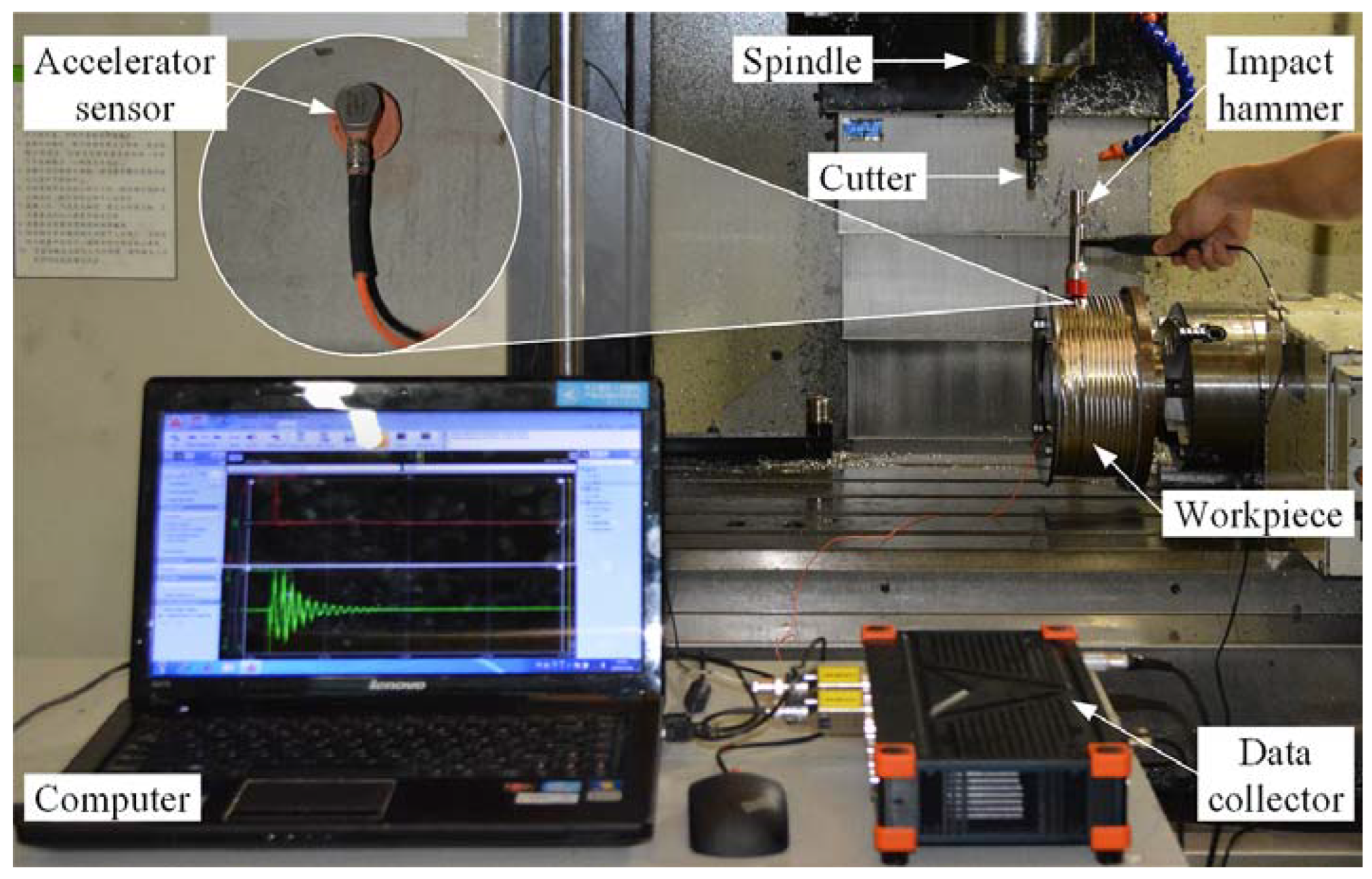
3.3. Dynamic Parameters

The modal parameters of the 3-DOF milling system along the x-axis, y-axis, and z-axis directions are important input parameters for the proposed model and need to be determined beforehand. The modal parameters of the bull-nose end mill respond to the dynamics of the cutter, the tool holder, and the machine spindle. Similarly, the modal parameters of the thin-walled cylinder respond to the dynamics of the workpiece, the fixture, and the machine table. In general, they are the integrated dynamic characteristics of the 3-DOF milling system. Therefore, the modal parameter results are dependent on the machine setup. A group of modal impact experiments is performed on the experimental setup, as demonstrated in Figure 9.
A Kistler 9722A impact hammer with a sensitivity of 10 mV/N is employed to produce the striking force. A Dytran 5225F1 accelerator sensor with a sensitivity of 10.04 mV/g is employed to collect the acceleration signals. The modal impact tests are performed 10 times along the x-axis, y-axis, and z-axis directions, respectively. The collected values are averaged to decrease random errors. The dynamic parameters of the 3-DOF milling system are determined by means of modal analysis. Table 4 presents the identified results.

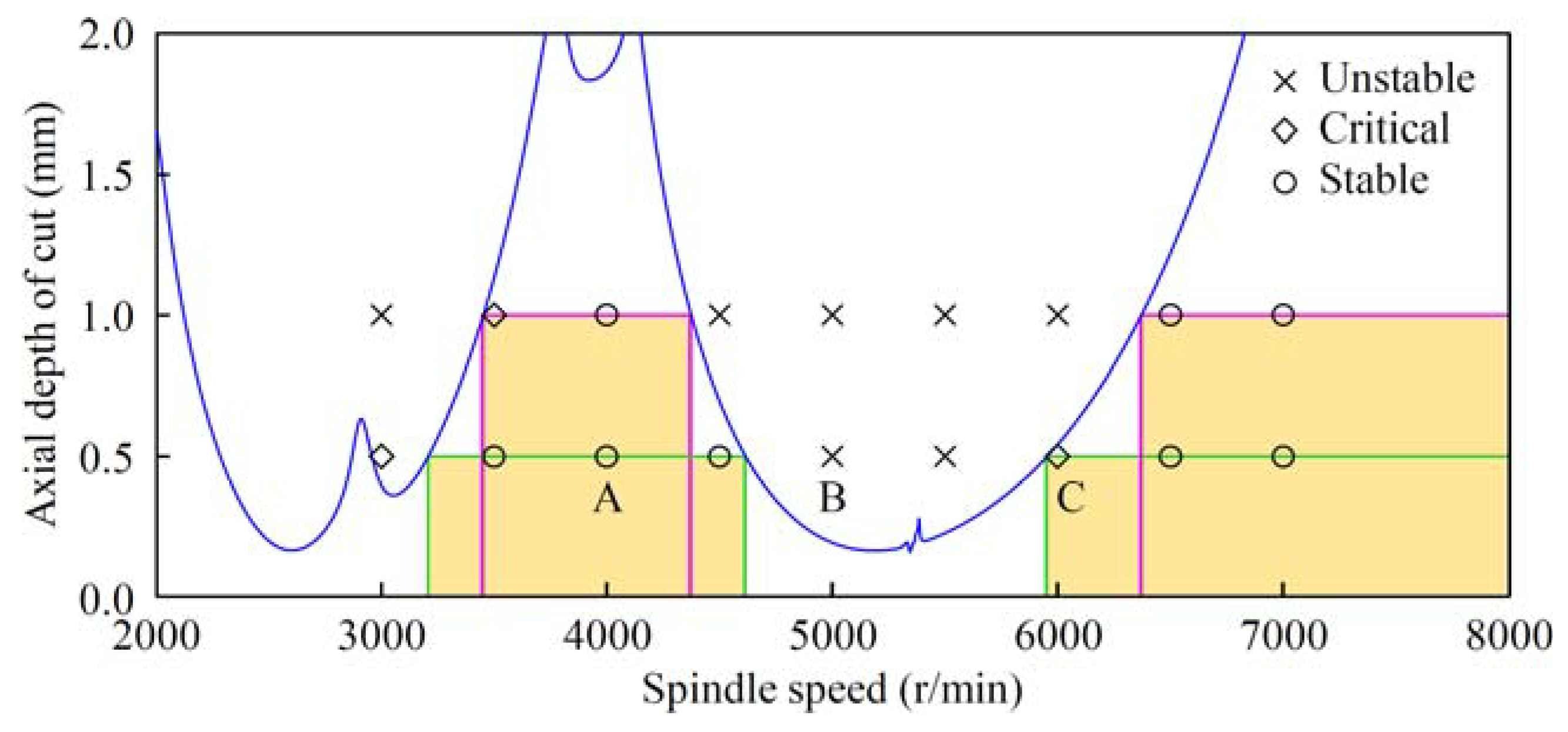
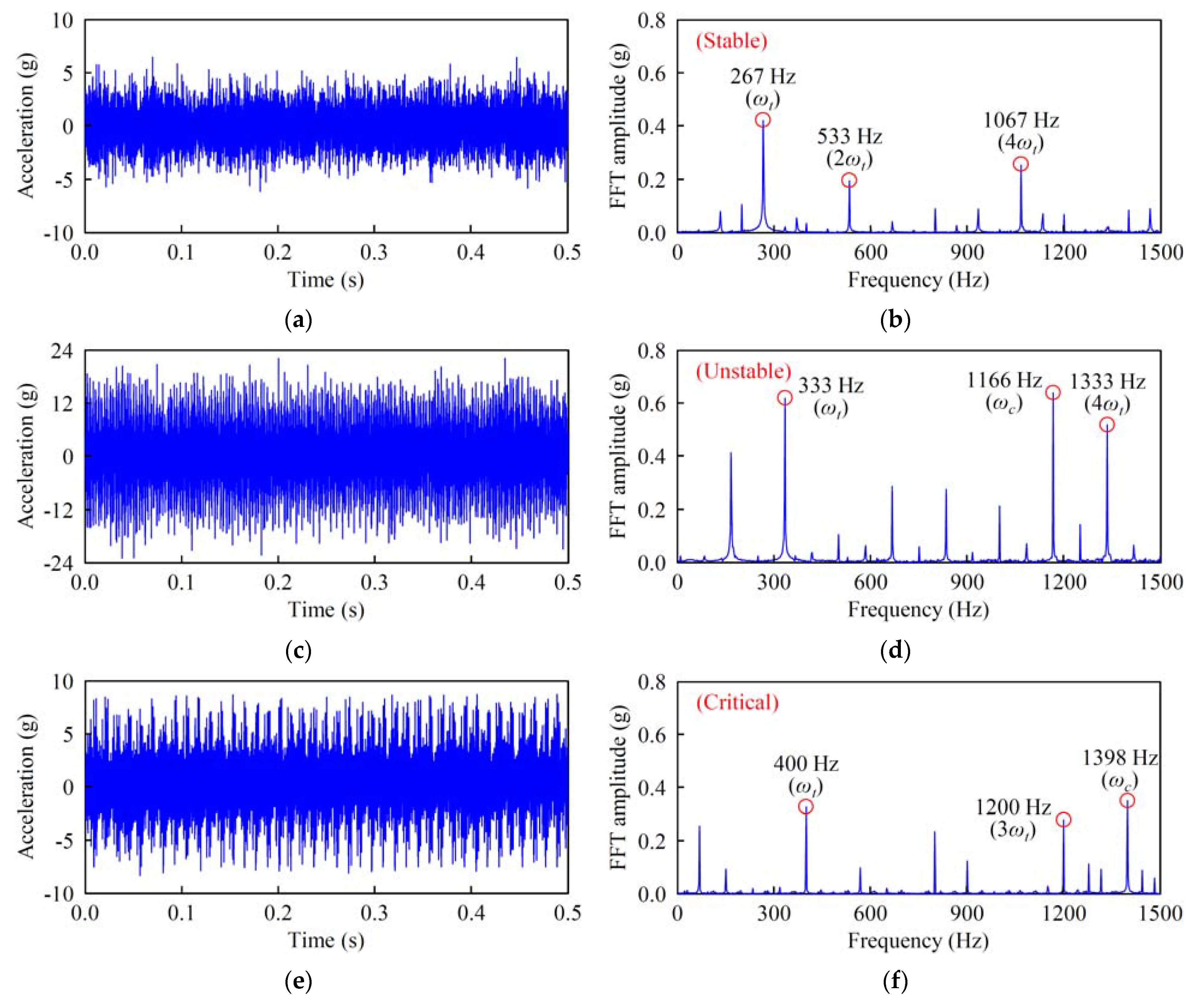
3.4. Chatter Stability Analysis and Experimental Validation

According to the SDM presented in Section 2.5, the SLD for bull-nose end milling of a thin-walled cylinder is calculated, as demonstrated in Figure 10.
The spindle speed varies within the interval from 2000 r/min to 8000 r/min. The axial depth of the cut varies within the interval from 0.0 mm to 2.0 mm. It can be found that there are three milling states: stable, critical, and unstable, which are distinguished by the stability boundary. The stable and unstable regions are below and above the stability boundary, respectively. The critical stable region is located near the stability boundary. For a depth of cut of 0.5 mm, the spindle speed within the intervals of 3204–4612 r/min and 5950–8000 r/min theoretically ensures stable milling. For a depth of cut of 1.0 mm, the spindle speed within the intervals of 3450–4372 r/min and 6369–8000 r/min theoretically ensures stable milling. However, the above ranges have to be contracted appropriately due to the critical stable region. In this paper, ±100 r/min is used to determine the critical stable region. Then, the spindle speed intervals for stable milling with a 0.5 mm axial depth of cut are 3304–4512 r/min and 6050–8000 r/min; the spindle speed intervals for stable milling with a 1.0 mm axial depth of cut are 3550–4272 r/min and 6469–8000 r/min.
For verifying the accuracy of the SLD, a group of bull-nose end milling tests are performed on a thin-walled cylinder, as demonstrated in Figure 9. The shared milling conditions are set as follows: the milling mode is down milling, the radial depth of cut is fixed at 6 mm, and the feed per tooth is fixed at 0.016 mm/tooth. Table 5 presents the remaining milling parameters.
The time domain and frequency domain acceleration signals corresponding to points A, B, and C are demonstrated in Figure 11. The spindle speeds at points A, B, and C are 4000 r/min, 5000 r/min, and 6000 r/min, respectively. The axial depths of the cut at points A, B, and C are all 0.5 mm. The bull-nose end milling state at point A is stable. The amplitude of the acceleration signal at point A is the smallest. And the spectral amplitude is primarily emphasized at the tooth passage frequency of 267 Hz and its multi-times-frequencies of 533 Hz and 1067 Hz. The bull-nose end milling state at point B is unstable. The amplitude of the acceleration signal at point B is the greatest. The corresponding spectrum has a chatter frequency of 1166 Hz, which is not an integral multiple of the tooth passage frequency of 333 Hz. The spectrum energy at the chatter frequency is greater than that at the tooth passage frequency. The bull-nose end milling state at point C is critical and stable. The amplitude of the acceleration signal is greater than that in the stable case but smaller than that in the unstable case. The chatter frequency of 1398 Hz occurs in the acceleration spectrum, whose energy is relatively low.
Figure 12 illustrates the finished surfaces of the thin-walled cylinder that correspond to the milling parameters at points A, B, and C in Figure 10. It can be clearly seen that significant chatter marks appear in the unstable case; slight chatter waves appear in the critical stable case; while in the stable case, the finished surface is sleek and its roughness (Ra) is very low.

4. Conclusions

Bull-nose end milling is an excellent finishing operation since it can provide greater material removal rates and smoother surface finishes. However, the regenerative chatter often occurs in the bull-nose end milling of thin-wall cylindrical parts, which have a ring-shaped and closed geometry structure. The dynamics of the cutter subsystem and the workpiece subsystem, the CWE, and the cutting force coefficients have a significant influence on the chatter stability. The objective of this article is to establish an accurate and applicable model to predict chatter stability during bull-nose end milling of thin-walled cylindrical parts. The main conclusions are summarized as follows:
(1)
A 3-DOF chatter stability model is developed, which is applicable to forecast the regenerative chatter in the bull-nose end finish milling of thin-walled cylindrical parts. It reflects the dynamics of the cutter subsystem in the x-axis and y-axis directions and the dynamic of the workpiece subsystem in the surface normal (namely, z-axis) direction. The SDM is employed to solve the dynamic equation describing the 3-DOF milling system;
(2)
A slice-intersection-based method for calculating the engagement boundary curve is established. The method is applicable to determining the CWE geometries with different milling conditions, such as slotting and following cuts. Furthermore, a lead angle of 0 degrees is recommended to maximize the machined strip width;
(3)
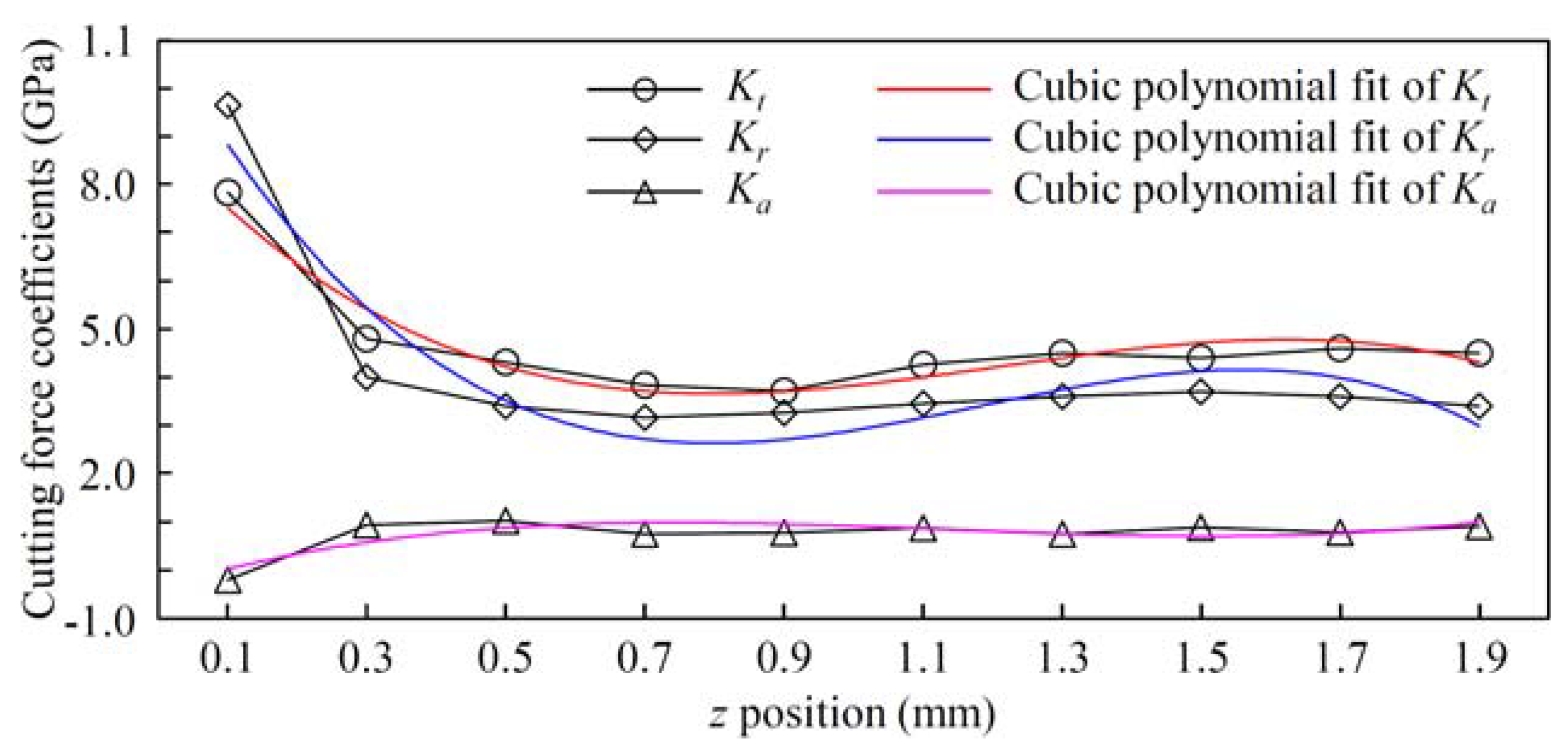
The approach to layered cutting force coefficient identification is presented considering the effect of varying cutter diameter. The specific coefficients for each cutting disk element can be determined by substituting the corresponding height into the cubic fitting polynomial;
(4)
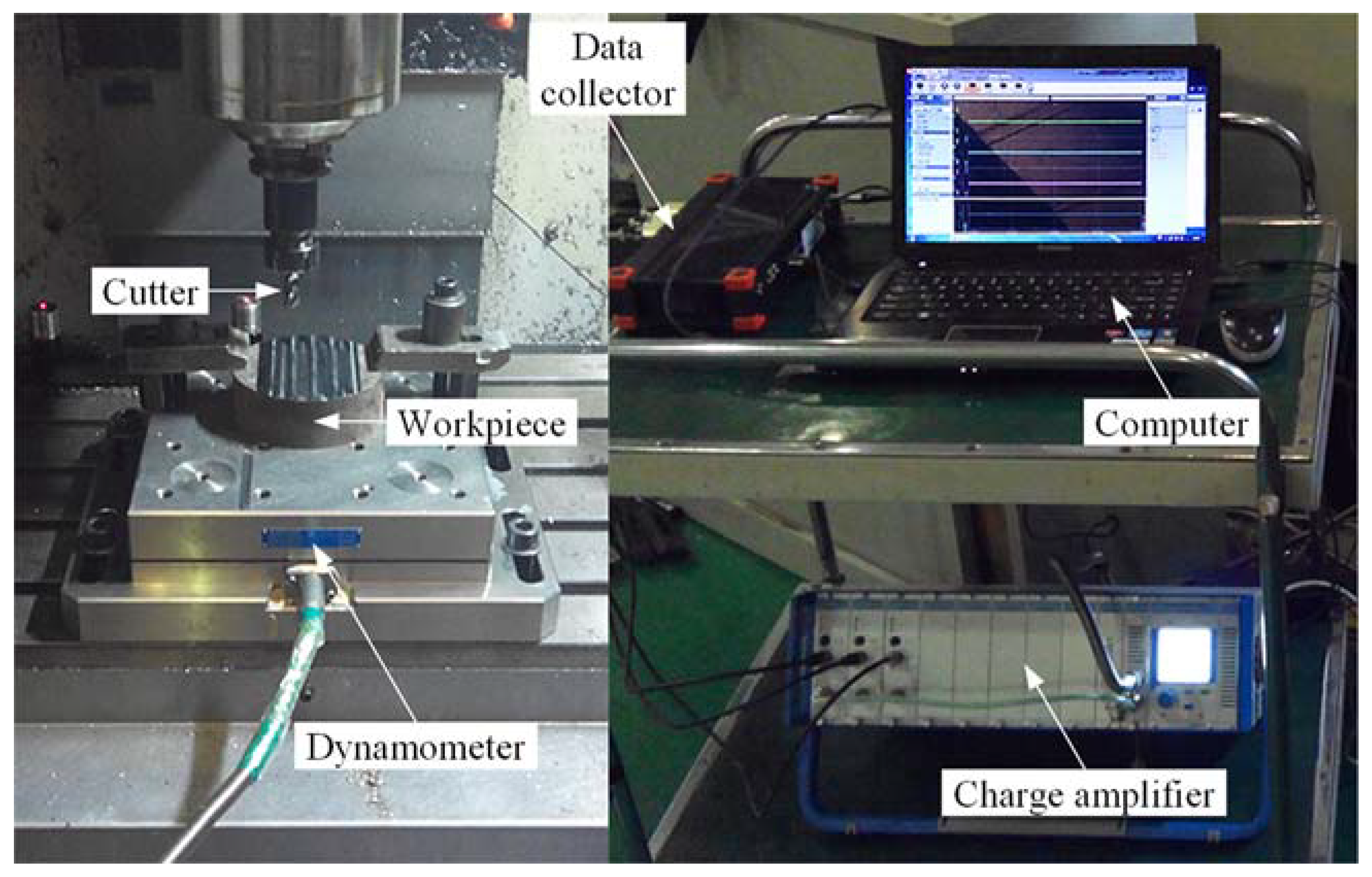
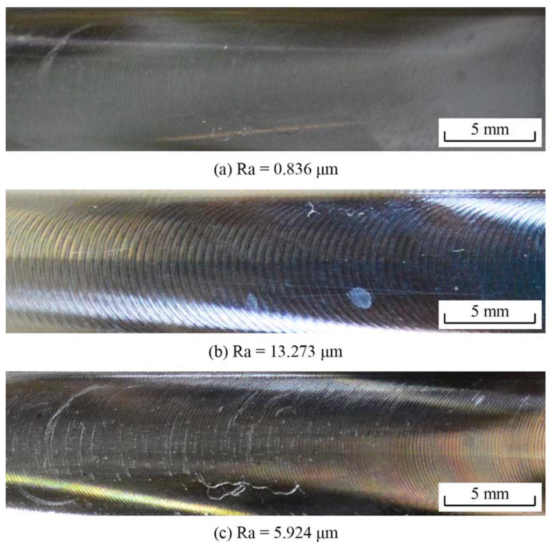
The validation tests of the proposed model are performed on a four-axis CNC machine tool. The predicted SLD agrees well with the experimental data. The spindle speed and the axial depth of the cut can be optimally chosen using the SLD to effectively avoid regenerative chatter and achieve smooth surfaces.

Author Contributions

Conceptualization, X.Z. and D.Z.; methodology, X.Z. and B.W.; software, X.Z.; validation, B.W.; formal analysis, C.Z. and D.Z.; data curation, X.Z. and M.X.; writing—original draft preparation, X.Z.; writing—review and editing, C.Z. and M.X.; funding acquisition, X.Z. and C.Z. All authors have read and agreed to the published version of the manuscript.

Funding

This research was supported by the National Key Research and Development Program of China, grant number 2020YFF0304905; and the research fund of the Key Laboratory of High Performance Manufacturing for Aero Engine (Northwestern Polytechnical University), Ministry of Industry and Information Technology, grant number HPM-2020-05.

Institutional Review Board Statement

Not applicable.

Informed Consent Statement

Not applicable.

Data Availability Statement

Not applicable.

Acknowledgments

The authors would like to thank Yongfeng Hou for calculating the CWEs and programming the toolpaths in Siemens NX 8.0 software.

Conflicts of Interest

The authors declare no conflict of interest.

References

  1. Dong, J.; Chang, Z.; Chen, P.; He, J.; Wan, N. Two-Dimensional Profile Simulation Model for Five-Axis CNC Machining with Bull-Nose Cutter. Appl. Sci. 2022, 12, 8230. [Google Scholar] [CrossRef]
  2. Fan, H.Z.; Xi, G.; Wang, W.; Cao, Y.L. An efficient five-axis machining method of centrifugal impeller based on regional milling. Int. J. Adv. Manuf. Technol. 2016, 87, 789–799. [Google Scholar] [CrossRef]
  3. Tang, X.; Zhu, Z.; Yan, R.; Chen, C.; Peng, F.; Zhang, M.; Li, Y. Stability Prediction Based Effect Analysis of Tool Orientation on Machining Efficiency for Five-Axis Bull-Nose End Milling. J. Manuf. Sci. Eng. 2018, 140, 121015. [Google Scholar] [CrossRef]
  4. Yue, C.; Gao, H.; Liu, X.; Liang, S.Y.; Wang, L. A review of chatter vibration research in milling. Chin. J. Aeronaut. 2019, 32, 215–242. [Google Scholar] [CrossRef]
  5. Du, X.; Ren, P.; Zheng, J. Predicting Milling Stability Based on Composite Cotes-Based and Simpson’s 3/8-Based Methods. Micromachines 2022, 13, 810. [Google Scholar] [CrossRef] [PubMed]
  6. Wan, M.; Zhang, W.H.; Dang, J.W.; Yang, Y. A unified stability prediction method for milling process with multiple delays. Int. J. Mach. Tools Manuf. 2010, 50, 29–41. [Google Scholar] [CrossRef]
  7. Altintas, Y.; Budak, E. Analytical Prediction of Stability Lobes in Milling. CIRP Ann. Manuf. Technol. 1995, 44, 357–362. [Google Scholar] [CrossRef]
  8. Budak, E.; Altintas, Y. Analytical Prediction of Chatter Stability in Milling—Part I: General Formulation. J. Dyn. Sys. Meas. Control. 1998, 120, 22–30. [Google Scholar] [CrossRef]
  9. Budak, E.; Altintas, Y. Analytical Prediction of Chatter Stability in Milling—Part II: Application of the General Formulation to Common Milling Systems. J. Dyn. Sys. Meas. Control. 1998, 120, 31–36. [Google Scholar] [CrossRef]
  10. Merdol, S.D.; Altintas, Y. Multi Frequency Solution of Chatter Stability for Low Immersion Milling. J. Manuf. Sci. Eng. 2004, 126, 459–466. [Google Scholar] [CrossRef]
  11. Zhu, L.; Liu, C. Recent progress of chatter prediction, detection and suppression in milling. Mech. Syst. Signal Process. 2020, 143, 106840. [Google Scholar] [CrossRef]
  12. Insperger, T.; Stépán, G. Updated semi-discretization method for periodic delay-differential equations with discrete delay. Int. J. Numer. Methods Eng. 2004, 61, 117–141. [Google Scholar] [CrossRef]
  13. Insperger, T.; Stépán, G.; Turi, J. On the higher-order semi-discretizations for periodic delayed systems. J. Sound Vib. 2008, 313, 334–341. [Google Scholar] [CrossRef]
  14. Jiang, S.; Sun, Y.; Yuan, X.; Liu, W. A second-order semi-discretization method for the efficient and accurate stability prediction of milling process. Int. J. Adv. Manuf. Technol. 2017, 92, 583–595. [Google Scholar] [CrossRef]
  15. Yan, Z.; Zhang, C.; Jia, J.; Ma, B.; Jiang, X.; Wang, D.; Zhu, T. High-order semi-discretization methods for stability analysis in milling based on precise integration. Precis. Eng. 2022, 73, 71–92. [Google Scholar] [CrossRef]
  16. Ding, Y.; Zhu, L.M.; Zhang, X.J.; Ding, H. A full-discretization method for prediction of milling stability. Int. J. Mach. Tools Manuf. 2010, 50, 502–509. [Google Scholar] [CrossRef]
  17. Ding, Y.; Zhu, L.M.; Zhang, X.J.; Ding, H. Second-order full-discretization method for milling stability prediction. Int. J. Mach. Tools Manuf. 2010, 50, 926–932. [Google Scholar] [CrossRef]
  18. Quo, Q.; Sun, Y.; Jiang, Y. On the accurate calculation of milling stability limits using third-order full-discretization method. Int. J. Mach. Tools Manuf. 2012, 62, 61–66. [Google Scholar] [CrossRef]
  19. Ma, J.; Li, Y.; Zhang, D.; Zhao, B.; Wang, G.; Pang, X. A Novel Updated Full-Discretization Method for Prediction of Milling Stability. Micromachines 2022, 13, 160. [Google Scholar] [CrossRef] [PubMed]
  20. Tang, X.; Peng, F.; Yan, R.; Gong, Y.; Li, Y.; Jiang, L. Accurate and efficient prediction of milling stability with updated full discretization method. Int. J. Adv. Manuf. Technol. 2017, 88, 2357–2368. [Google Scholar] [CrossRef]
  21. Yan, Z.; Wang, X.; Liu, Z.; Wang, D.; Jiao, L.; Ji, Y. Third order updated full-discretization method for milling stability prediction. Int. J. Adv. Manuf. Technol. 2017, 92, 2299–2309. [Google Scholar] [CrossRef]
  22. Herranz, S.; Campa, F.J.; López de Lacalle, L.N.; Rivero, A.; Lamikiz, A.; Ukar, E.; Sánchez, J.A.; Bravo, U. The milling of airframe components with low rigidity: A general approach to avoid static and dynamic problems. Proc. Inst. Mech. Eng. Part B J. Eng. Manuf. 2005, 219, 789–801. [Google Scholar] [CrossRef]
  23. Fei, J.; Xu, F.; Lin, B.; Huang, T. State of the art in milling process of the flexible workpiece. Int. J. Adv. Manuf. Technol. 2020, 109, 1695–1725. [Google Scholar] [CrossRef]
  24. Dong, H.; Ji, Y.; Wang, X.; Bi, Q. Stability analysis of thin-walled parts end milling considering cutting depth regeneration effect. Int. J. Adv. Manuf. Technol. 2021, 113, 3319–3328. [Google Scholar] [CrossRef]
  25. Campa, F.J.; López de Lacalle, L.N.; Lamikiz, A.; Sánchez, J.A. Selection of cutting conditions for a stable milling of flexible parts with bull-nose end mills. J. Mater. Process. Technol. 2007, 191, 279–282. [Google Scholar] [CrossRef]
  26. Campa, F.J.; López de Lacalle, L.N.; Celaya, A. Chatter avoidance in the milling of thin floors with bull-nose end mills: Model and stability diagrams. Int. J. Mach. Tools Manuf. 2011, 51, 43–53. [Google Scholar] [CrossRef]
  27. Seguy, S.; Campa, F.J.; López de Lacalle, L.N.; Arnaud, L.; Dessein, G.; Aramendi, G. Toolpath dependent stability lobes for the milling of thin-walled parts. Int. J. Mach. Mach. Mater. 2008, 4, 377–392. [Google Scholar] [CrossRef]
  28. Puma-Araujo, S.D.; Olvera-Trejo, D.; Martinez-Romero, O.; Urbikain, G.; Elías-Zúñiga, A.; López de Lacalle, L.N. Semi-Active Magnetorheological Damper Device for Chatter Mitigation during Milling of Thin-Floor Components. Appl. Sci. 2020, 10, 5313. [Google Scholar] [CrossRef]
  29. Zhou, X.; Zhang, D.; Luo, M.; Wu, B. Chatter stability prediction in four-axis milling of aero-engine casings with bull-nose end mill. Chin. J. Aeronaut. 2015, 28, 1766–1773. [Google Scholar] [CrossRef]
  30. Adetoro, O.B.; Sim, W.M.; Wen, P.H. An improved prediction of stability lobes using nonlinear thin wall dynamics. J. Mater. Process. Tech. 2010, 210, 969–979. [Google Scholar] [CrossRef]
  31. Fei, J.; Lin, B.; Yan, S.; Zhang, X.; Lan, J.; Dai, S. Chatter prediction for milling of flexible pocket-structure. Int. J. Adv. Manuf. Technol. 2017, 89, 2721–2730. [Google Scholar] [CrossRef]
  32. Gu, D.; Wei, Y.; Xiong, B.; Liu, S.; Zhao, D.; Wang, B. Three degrees of freedom chatter stability prediction in the milling process. J. Mech. Sci. Technol. 2020, 34, 3489–3496. [Google Scholar] [CrossRef]
  33. Yan, R.; Gong, Y.; Peng, F.; Tang, X.; Li, H.; Li, B. Three degrees of freedom stability analysis in the milling with bull-nosed end mills. Int. J. Adv. Manuf. Technol. 2016, 86, 71–85. [Google Scholar] [CrossRef]
  34. Dang, X.B.; Wan, M.; Zhang, W.H.; Yang, Y. Stability analysis of the milling process of the thin floor structures. Mech. Syst. Signal Process. 2022, 165, 108311. [Google Scholar] [CrossRef]
  35. Yu, G.; Wang, L.; Wu, J. Prediction of chatter considering the effect of axial cutting depth on cutting force coefficients in end milling. Int. J. Adv. Manuf. Technol. 2018, 96, 3345–3354. [Google Scholar] [CrossRef]
  36. Adetoro, O.B.; Sim, W.M.; Wen, P.H. Stability Lobes Prediction for Corner Radius End Mill Using Nonlinear Cutting Force Coefficients. Mach. Sci. Technol. 2012, 16, 111–130. [Google Scholar] [CrossRef]
  37. Altintas, Y. Manufacturing Automation: Metal Cutting Mechanics, Machine Tool Vibrations, and CNC Design, 2nd ed.; Cambridge University Press: Cambridge, UK, 2012. [Google Scholar]
  38. Yang, Y.; Liu, Q.; Zhang, B. Three-dimensional chatter stability prediction of milling based on the linear and exponential cutting force model. Int. J. Adv. Manuf. Technol. 2014, 72, 1175–1185. [Google Scholar] [CrossRef]
  39. Bedi, S.; Ismail, F.; Mahjoob, M.J.; Chen, Y. Toroidal versus ball nose and flat bottom end mills. Int. J. Adv. Manuf. Technol. 1997, 13, 326–332. [Google Scholar] [CrossRef]
  40. Fan, W.; Ye, P.; Zhang, H.; Fang, C.; Wang, R. Using rotary contact method for 5-axis convex sculptured surfaces machining. Int. J. Adv. Manuf. Technol. 2013, 67, 2875–2884. [Google Scholar] [CrossRef]
  41. Gradišek, J.; Kalveram, M.; Weinert, K. Mechanistic identification of specific force coefficients for a general end mill. Int. J. Mach. Tools Manuf. 2004, 44, 401–414. [Google Scholar] [CrossRef]
  42. Gao, G.; Wu, B.; Zhang, D.; Luo, M. Mechanistic identification of cutting force coefficients in bull-nose milling process. Chin. J. Aeronaut. 2013, 26, 823–830. [Google Scholar] [CrossRef]
Figure 1. 3-DOF dynamic model in bull-nose end milling of a thin-walled cylinder.
Applsci 13 06737 g001
Figure 2. Geometry of a bull-nose end cutter.
Applsci 13 06737 g002
Figure 3. CWE at a cutting contact point.
Applsci 13 06737 g003
Figure 4. Calculation of CWE boundary 1. (a) Calculation of the intersection curve between each slice and the cutter toroidal surface; (b) Calculation of the two boundary points on the intersection curve.
Applsci 13 06737 g004
Figure 5. Flowchart of CWE calculation.
Applsci 13 06737 g005
Figure 6. Calculated CWEs for the following cut with a radial depth of cut of 6 mm and axial depth of cut of 0.5 mm. (a) Effect of lead angle on the CWE maps; (b) Three-dimensional CWE in the CCS with a lead angle of 0 degrees.
Applsci 13 06737 g006
Figure 7. Experimental setup for the slotting experiments.
Applsci 13 06737 g007
Figure 8. Layered cutting force coefficients.
Applsci 13 06737 g008
Figure 9. Modal impact tests and milling tests.
Applsci 13 06737 g009
Figure 10. Predicted SLD.
Applsci 13 06737 g010
Figure 11. Time-domain and frequency-domain analysis of acceleration signals at each point. (a) Acceleration at point A; (b) FFT for acceleration at point A; (c) Acceleration at point B; (d) FFT for acceleration at point B; (e) Acceleration at point C; (f) FFT for acceleration at point C.
Applsci 13 06737 g011
Figure 12. Finished surfaces of the thin-walled cylinder. (a) Finished surface at point A, Ra = 0.836 μm; (b) Finished surface at point B, Ra = 13.273 μm; (c) Finished surface at point C, Ra = 5.924 μm.
Applsci 13 06737 g012
Table 1. Cutter specifications.
Cutter TypeCutter MaterialNumber of FlutesDiameter
(mm)
Fillet Radius
(mm)
Helix Angle
(°)
Overhang
(mm)
Bull-nose end mill3 μm TiAlN-coated carbide41223875
Table 2. Workpiece parameters.
Workpiece
Material
Geometries (mm)Density
(kg/m3)
Young’s
Modulus (GPa)
Poisson’s
Ratio
Inner DiameterOuter DiameterHeight
06Cr19Ni102112179079301940.3
Table 3. Machining parameters used in the slotting tests.
Spindle Speed
(r/min)
Feed Rate per Tooth
(mm/tooth)
Axial Depth of Cut
(mm)
50000.008, 0.016, 0.024, 0.0320.2, 0.4, 0.6, 0.8, 1.0,
1.2, 1.4, 1.6, 1.8, 2.0
Table 4. Modal parameters.
CasesFrequency
(Hz)
Damping
(%)
Stiffness
(N/m)
Cutter (x-axis)17682.61.85 × 108
Cutter (y-axis)17532.31.79 × 108
Workpiece (z-axis)7943.64.25 × 107
Table 5. Stability states with different milling conditions.
No.Spindle Speed
(r/min)
Feed Rate
(mm/min)
Axial Depth of Cut
(mm)
Stability State
130001920.5Critical
230001921.0Unstable
335002240.5Stable
435002241.0Critical
540002560.5Stable
640002561.0Stable
745002880.5Stable
845002881.0Unstable
950003200.5Unstable
1050003201.0Unstable
1155003520.5Unstable
1255003521.0Unstable
1360003840.5Critical
1460003841.0Unstable
1565004160.5Stable
1665004161.0Stable
1770004480.5Stable
1870004481.0Stable
Disclaimer/Publisher’s Note: The statements, opinions and data contained in all publications are solely those of the individual author(s) and contributor(s) and not of MDPI and/or the editor(s). MDPI and/or the editor(s) disclaim responsibility for any injury to people or property resulting from any ideas, methods, instructions or products referred to in the content.

