Power Transformer Condition-Based Evaluation and Maintenance (CBM) Using Dempster–Shafer Theory (DST)

Abstract

Transformers are the most important elements in the power system. Due to their mass and complexity, they require constant monitoring and maintenance. Maintenance of power transformers increases the availability of the power system. The large number of substations and the specifics of their locations make condition-based maintenance (CBM) useful as part of the system’s on-demand response. Unlike other system responses, the transformer contains a large amount of uncertain information, both qualitative and numerical. A large amount of information is necessary to implement CBM, but due to the often incomplete information, an analysis tool is essential. In this paper, a multi-level condition assessment framework based on evidential reasoning is proposed. A model for condition-based maintenance of a power transformer and procedures for the aggregation process based on evidential reasoning are presented. The implementation of the decomposition model with appropriate weights of a baseline and general attributes was made. Based on the decomposition model, the data and ratings of baseline attributes were collected. By carrying out the aggregation process, the ratings of the baseline attributes, as well as the ratings of the condition of the individual elements and the overall rating of the system condition as a whole, for several points in time, were obtained. The scientific contribution of the work is the proposal of an analysis that provides an insight into the condition of a complex technical system based on a single numerical value, thus determining its priority in the maintenance process.

1. Introduction

World economy and energy production trends also affect the power grid, plant management and maintenance techniques. Those trends greatly contribute to mergers of companies with different infrastructure, strategies and IT support. Such companies own plants of various conditions, some well past their prime, but seldom brand new. In an environment where the price of production is subject to market competition on a global level, it is necessary to find an optimum or a compromise between investments in the development, reconstruction and maintenance of facilities, on the one hand, and the market price of products or services, on the other hand. When choosing the appropriate maintenance method, the documentation on the plant’s behavior, the database or knowledge base on the types of faults, their frequency, as well as the service life of each part or the entire plant, proved to be particularly useful. A digitalized knowledge base with an appropriate information system and the necessary tools for analyzing existing data enables simpler decision-making based on objective information and with less of a labor force needed. For this purpose, special software packages that enable simpler and more efficient plant management are being developed. By connecting such tools with the plant management system, it is possible to document the measures taken and later, analyze the fidelity of the decisions made followed by the accompanying consequences on the plant or production process [1,2,3].

Efficient plant maintenance leads to a reduction in production costs and the conservation of resources. Technical maintenance is necessary for ensuring the system’s operating efficiency and attaining the desired performance. Since the operation and maintenance costs of technical equipment and systems might range from 15 to 30% of the lifespan cost, they are not eligible. As a result, managing and reducing maintenance costs has become increasingly important to academics, stakeholders and operators. Ordinarily, the increase in efficiency can be achieved by continuous collection and classification of data for observed object and its components to increase reliability and reduce mandatory maintenance measures, implementing strategies for better organization of operation and maintenance, transparency of operations, displaying all costs and evaluation of the justification of individual investments. The successful implementation of the above requires up-to-date knowledge of the technical and economic conditions of plant operation, access to and the analysis of a large amount of information and collected data; therefore, the existence of an efficient information system based on modern hardware and software solutions is necessary.

The process of exploitation of the technical system is disrupted by the degradation of its performance. To maintain the level of production, negative changes in the technical system must be prevented by certain countermeasures in order to restore the original operability of the system. The measures taken in this case are considered maintenance. The definition of maintenance as a technological procedure can be defined as the measures necessary for the preservation and restoration of the nominal condition of the object or procedures related to the determination and assessment of the current condition of technical objects and systems, which includes prevention, diagnosis, condition analysis and repair. Norm DIN 31 051 addresses maintenance activities such as servicing, inspection and repair [4].

There are several characteristic methods of maintaining technical systems: Condition Based Maintenance (CBM), Reliability Centered Maintenance, Lean Maintenance, Total Lifecycle Costs Strategy and Total Productive Maintenance [5]. A quality maintenance strategy for a system must be chosen according to its needs and it most often represents a combination of the aforementioned methods. The maintenance strategy must consider operational losses caused by breakdowns, reduction of total maintenance and organizational costs. The purpose of the chosen strategy is to fulfill the maintenance target functions as best as possible. The target functions are usually related to increasing the system usability, ensuring a certain degree of reliability, optimizing the number of employees, reducing the total cost, etc. 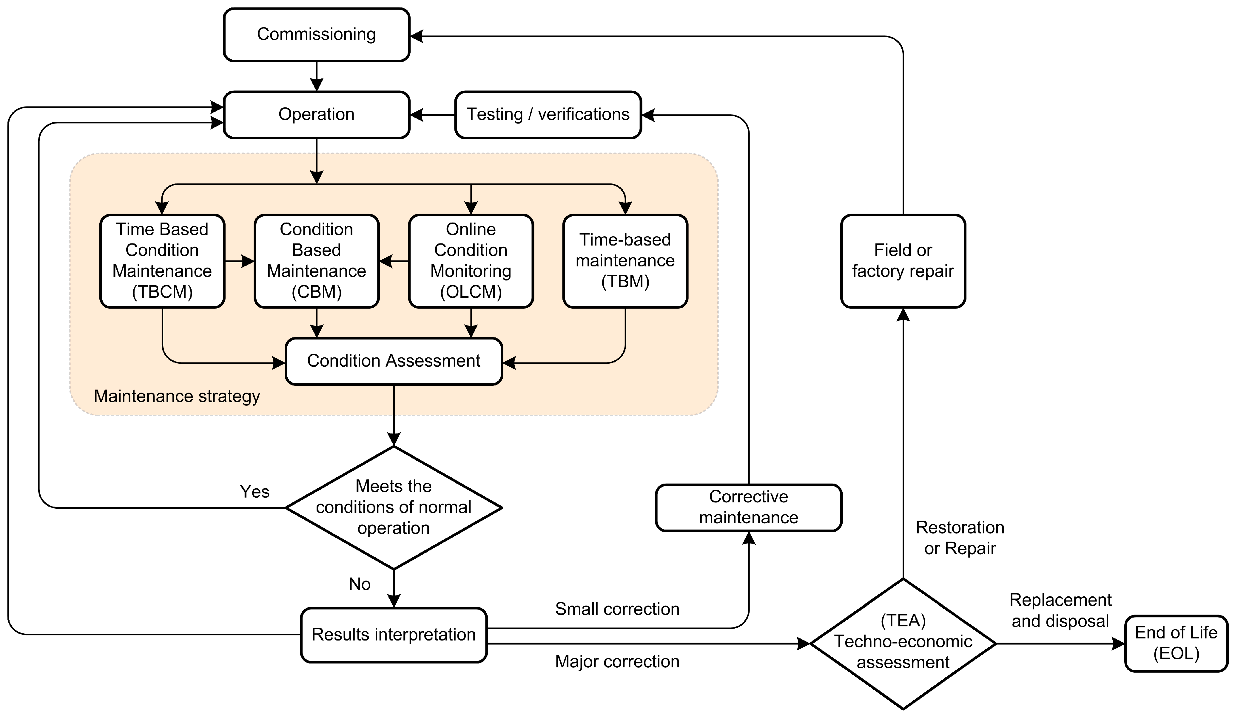Figure 1 Presents a typical maintenance procedure. The general issue of the maintenance strategy is opting for maintenance before or after the fault occurrence. Figure 1 shows a general maintenance strategy diagram.

The general issue of the maintenance strategy is opting for maintenance before or after the fault occurrence.

Maintenance after the fault occurrence (Failure maintenance, Breakdown maintenance) operates after a fault and depends on its type and severity. With this type of maintenance, there are no preventive actions. Malfunctions or errors usually lead to a stoppage of the entire system and/or an interruption in its operation. The disadvantage of this approach is the unpredictability of the duration, type of necessary repairs and the possibility of secondary damage or damage to other parts of the system caused by the initial fault.

Periodic maintenance (time-based maintenance) represents a systematic approach to system maintenance where actions are planned and take place at certain time intervals. If a fault occurs within the period between two scheduled interventions, only minimal interventions are performed to return the system to a functional condition. The best example of this method is a thermal energy production and distribution system with a critical period for the operation of the heating system being the winter season. With this system, the best time for shutdown, maintenance, overhaul and preparation of the system for a new cycle is outside the heating season, i.e., summer and autumn. The advantage of periodic maintenance is that all interventions as well as the time required for regular maintenance are planned. The disadvantage of this approach lies in the fact that the cycle length is predicted based on statistical indicators, thus, this can lead to an excessively long cycle. This approach can ensure very high reliability and availability of the maintained system, which is naturally accompanied by high maintenance costs.

Condition based maintenance is a combination of the two above-mentioned approaches, i.e. periodic maintenance and maintenance after a fault [6,7,8,9,10]. The idea is to use the advantages of the latter, that is, to use the reserves of components and parts of the system as much as possible and, at the same time, avoid the disadvantages of periodic maintenance. Maintenance according to the system condition uses all available methods to determine the technical level of the system and equipment condition to access maintenance only when the condition of system components falls below a certain critical level. The condition of the system is determined by tests, inspections, diagnosis, measurement and the analysis of measured data [11,12,13]. The advantages of this approach are high reliability and maximum utilization of system parts reserves. The disadvantages are that the system depends on the ability to perform adequate measurements and the reliability of system diagnosis. In addition, since the time for carrying out the overhaul is not planned but depends exclusively on the condition of the system, the execution of major procedures on the system may fall at an inappropriate time, i.e., time when the market demands high availability of the system.

When making decisions regarding maintenance based on risk assessment, we distinguish between two types of risks. The first would be a risk in terms of the safety and reliability of production and risk in estimating the cost of system maintenance and production maintenance. The risk related to the assessment of the cost of maintenance and operation can be expressed as the product of the frequency of fault and the amount of its consequent damage. Equation (1) shows risk R for carrying out or not carrying out maintenance, where H is the frequency of fault occurrences or irregularities and S represents the level of potential damage. The frequency of faults H is determined with the help of statistical methods and reliability theory, while the level of damage S is determined as the cost of production downtime plus the cost of maintenance or the cost of repairing of fault. The total amount of risk for a system represents the sum of risks for each part of the system:

$$R={\displaystyle \sum }_{\mathrm{i}=1}^n{R}_i={\displaystyle \sum }_{\mathrm{i}=1}^n{S}_i\cdot H_i$$

(1)

where R_i represents risk for the i-th component, S_i the inherent cost and H_i the frequency of the fault on the i-th component.

The cost related to a single component of the system is defined as the cost, i.e., the cost of production downtime and the cost of repairs through the following equation:

$$S_i{=\mathrm{W}}_s\cdot t_i\cdot L_i+{\mathrm{K}}_i$$

(2)

where S_i represents the cost tied to the i-th component, W_s the value of the unit loss in the system downtime state, t_i the time needed for the component to be fixed, L_i the the amount of unit losses and K_i the cost of repairs.

The estimate of the frequency of faults is made on the basis of data on previous faults; therefore, it cannot be considered reliable. In addition, information from equipment manufacturers is often unavailable or difficult to use in a real work environment. From a security point of view, it is necessary to use a different and more complex data analysis than the one shown. Special attention should be paid to distinguishing between the individual system components in terms of exposure to risk, as a small number of components significantly affects the amount of the overall risk.

In modern technical facilities and enterprises, CBM has become a leading maintenance strategy in contrast to more traditional solutions relying on time-based maintenance. An optimal CBM strategy has the potential to provide significant benefits, increasing system availability, reducing maintenance costs and increasing product quality. A literature review [9] provides a detailed insight into theoretical foundations, specific implementations and operational aspects as well as future research directions. Theoretical and practical development in the field of general CBM and its current state of the art are in detail presented [10] and acknowledged.

The condition assessment is of great importance for the oil immersed type power transformers. Several methods for assessment of key parameters of the power transformer are well established and documented. They can be divided into two major groups, offline methods and online methods, each consisting of specific methods [14,15]. Common offline methods are determination of the degree of polymerization (DP), furan analysis, dielectric response analysis, insulation resistance, sweep frequency response analysis (SFRA) and others [11,16]. Online methods are dissolved gas analysis (DGA), partial discharge analysis, thermal monitoring and vibration analysis [11,15,17]. DGA is the most widely applied technique in modern monitoring systems and the application can be achieved either online or offline.

After offline or online measurement and data acquisition procedures, several methods can be used in order to determine overall condition or state of power transformer [16,18,19].

Described methods may include complex computational and/or artificial intelligence methods [12,13,19,20,21] (machine learning, artificial neural networks, fuzzy logic, etc.).

However, existing methods are often limited with the input information, their focus on a specific data set, their inability to assess the overall condition of the power transformer and a lack of the possibility to handle incomplete or uncertain data.

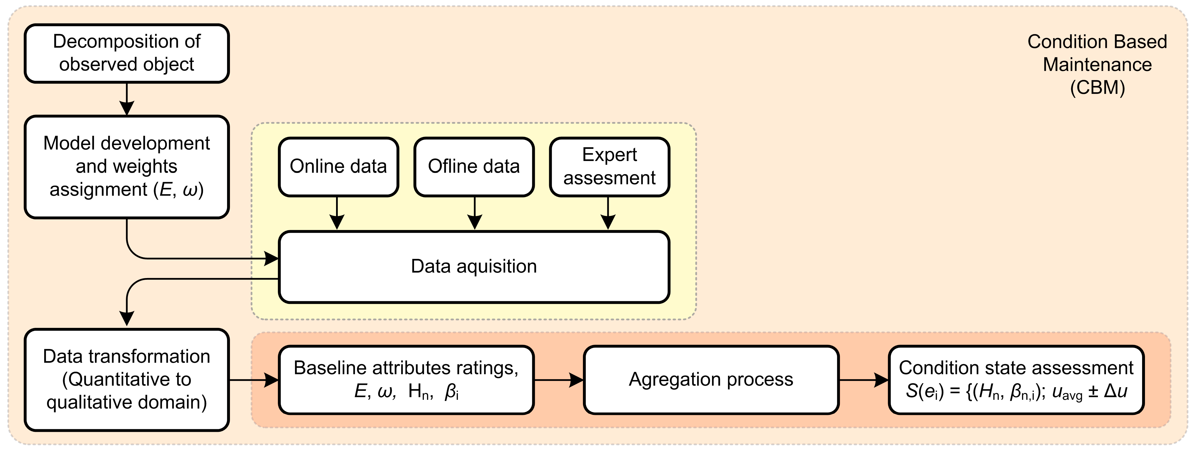
The solution presented in this paper proposes condition-based assessment and maintenance based on multiple attribute analysis and an evidential reasoning algorithm. The first step is to perform a decomposition of a desired object from general up to elementary attributes, determine weights for all attributes, collect offline and online data, convert collected quantitative data to qualitative grades, perform an aggregation process with attribute grades, weights and uncertainty and finally, obtain a single value, which represents the current condition state of the observed object. This utility grade is essential for a decision-making process regarding maintenance.

This paper is structured into four sections. Section 1, the Introduction, presents the current state of the CMB and power transformer maintenance procedures. Section 2 briefly describes the methodology used, while Section 3 elaborates on the evidential reasoning algorithm, decomposition and aggregation process for power transformer condition assessment. Section 4 gives a conclusion and recommendations for future work and development.

2. Methodology

The paper aims to provide an insight into the maintenance of complex technical systems by assessing their condition with special reference to power transformers. Power transformers are the basis of the power system. Unlike other power system elements, the unavailability of transformers, due to their characteristics, calls into question the availability of the power system as a whole. Transformer protection and transformer condition are the primary factors in the reliability of an electricity supply. Their maintenance, like that of most equipment, was historically carried out periodically as time-based maintenance. Due to the increased availability of the system, it has become more common to maintain the equipment by assessing its condition. For this reason, this paper defines certain types of necessary maintenance activities and the concept of equipment maintenance by assessing their condition. Dempster–Shafer theory (DST) [22] was used to implement maintenance by assessing the condition with incomplete information. For a successful implementation, it is necessary to define the algorithm of evidence-based inference and the possibility of its implementation. Realization of this task requires the creation of a decomposition model with appropriate weights of a baseline and general attributes. Based on the decomposition model, it is necessary to collect data and ratings of baseline attributes. Carrying out the aggregation process over the collected ratings of the baseline attributes for several time points determines the condition ratings and the overall condition rating for all available time points. The baseline hypothesis of the work is that the condition of a complex technical system can be represented by a single numerical value (or an ordered set of values) that represents a qualitative assessment of the system condition. Based on the assessment, one can gain an insight into the system condition and decide to continue with exploitation or to perform maintenance. The scientific contribution of the work is reflected in the proposal of a power transformer condition model suited for maintenance purposes by assessing the condition based on collected data and determining the condition of the system as a function of time and exploitation conditions using the aggregation procedure.

2.1. Maintenance Activities and System Decomposition

An industrial plant is a complex system made up of several subsystems or individual parts, i.e., components. The condition of each part directly affects the overall condition of the system.

It is important to note that such a complex object consists of several different subsystems that can again be divided into simpler systems or devices until the lowest level, object or device is reached. Each of the objects divided in this way affects the behavior of the entire system with a certain weight. To choose the most favorable approach to maintain, it is necessary to properly decompose the observed plant, that is, to disassemble the complex system into simpler parts from the maintenance point of view. Various approaches to decomposition are possible and decomposition is most often performed by an expert, i.e., a person with a high degree of knowledge about the production process, operation and maintenance of the observed system. The first division that can be made is the division of the system by priorities. This implies dividing the equipment into classes according to the degree of factual necessity of the system. In the simplest case, this means dividing the parts of the system into two classes, parts essential for the operation of the system and non-essential parts, i.e., equipment without which the system can work at least for a while. This division could be simply done based on empirical data for the observed system.

A more detailed division of the system into appropriate classes can be performed according to the consequences of a possible system, part of the system or individual equipment fault. That being said, the system parts can be divided into five classes as follows:

• system or system parts, the failure of which can lead to a complete stoppage of the plant;
• system or system parts, the failure of which significantly reduces the overall safety of the plant or may cause the fault of other system parts;
• system or system parts, the failure of which leads to a reduction in the operation level;
• system or system parts, the failure of which affects the reduction of the efficiency of the main production process;
• system or system parts whose failure does not have a direct impact on the production process.

This division of the system has proven to be a useful approach for various industrial segments, especially for facilities related to electricity production, transmission and distribution [12,23,24,25,26].

In the case of a system with a high frequency of faults or high sensitivity to them, the system can be classified according to system maintenance procedures instead of classification according to its parts. One of the possible divisions would be the following:

• maintenance carried out by the first free person;
• maintenance carried out within thirty minutes;
• maintenance carried out in the first free period;
• maintenance carried out within 3 months.

2.2. Condition Assessment Equipment Maintenance

Condition-based maintenance of technical objects or systems is based on the current physical or parametric condition of the observed object. This approach to maintenance is quite demanding due to the necessity of regular inspections and monitoring of the observed object or system. It is important to point out that by using this approach, the optimal utilization of the object life cycle is achieved.

2.2.1. Baseline Condition Assessment Maintenance Model

The condition assessment of the observed object is carried out on-site or remotely with the help of equipment for remote inspection and monitoring of the system. With advances in communication and information technology, equipment for remote monitoring of technical systems has become available and affordable to regular businesses. An analysis of the funds invested in equipment for remote monitoring and an analysis of the opportunities and services obtained in this way confirms the profitability of such investments. Information and quantities essential for the operation and maintenance of the technical system must be collected frequently and sometimes continuously. If such quantities can be measured in a relatively simple way, it can be concluded that the system is suitable for continuous intelligent monitoring, i.e., continuous collection of information about the operation and condition of the system with the help of equipment for measuring, remote reading and transmitting collected data. Such information is collected, locally processed and formulated, and then transferred to the central part of the monitoring system where further processing of the collected data is performed. Complex methods and algorithms for the analysis, processing and storage of collected data are available in the central part of the system for monitoring and processing collected information [27,28]. Figure 2 shows specific CBM steps.

2.2.2. Data Acquisition

Despite modern equipment developed for system monitoring, there is certain information about the system that, due to the complex measurement procedure or the very nature of the information, cannot be collected in this way, for example, the condition of the seals, general condition of the object, corrosion degree, etc. To collect these types of information, the participation of trained and experienced personnel who can perform inspections and measurements or provide an assessment of the condition of the object or system is required. Considering the way of collecting information, we can say that there are two different types of data. The first type of data collected is a dynamic information and as such, is collected with the help of equipment for remote monitoring, data collection, and transmission [7,17,19,29]. Another type of data is static information that is obtained on the spot, that is, by measurement or assessment by an expert on the system itself.

Based on collected information, dynamic or static, decisions are made about system maintenance [6,10,14,15,30,31]. The collected information is appropriately processed and interpreted [3,18]. The analysis of the objects’ condition shows that the condition of a certain observed object most often depends on the condition of several different attributes and that to determine the current condition of the object, it is necessary to use a decision analysis based on multiple attributes, i.e., Multiple Decision Data Analysis (MADA) [20,32,33] combined with evidential reasoning [2,22,34].

3. Evidential Reasoning Algorithm

In order to correctly evaluate the condition of the technical system, it is necessary to consider a large amount of numerical and qualitative data during the calculation process. For the purpose of interpreting numerical and qualitative values, it is necessary to use the appropriate semantics, i.e., the appropriate computing device.

3.1. Maintenance Activities and System Decomposition

The outcome of the technical system condition assessment is predetermined and classified with a certain degree of confidence in the accuracy of the assigned rating. Based on the condition assessment, a decision is made on the action to be taken, i.e., on the existence of the need for maintenance. The aim of maintenance is to raise the condition of the technical system to a higher level if the current condition is critically low.

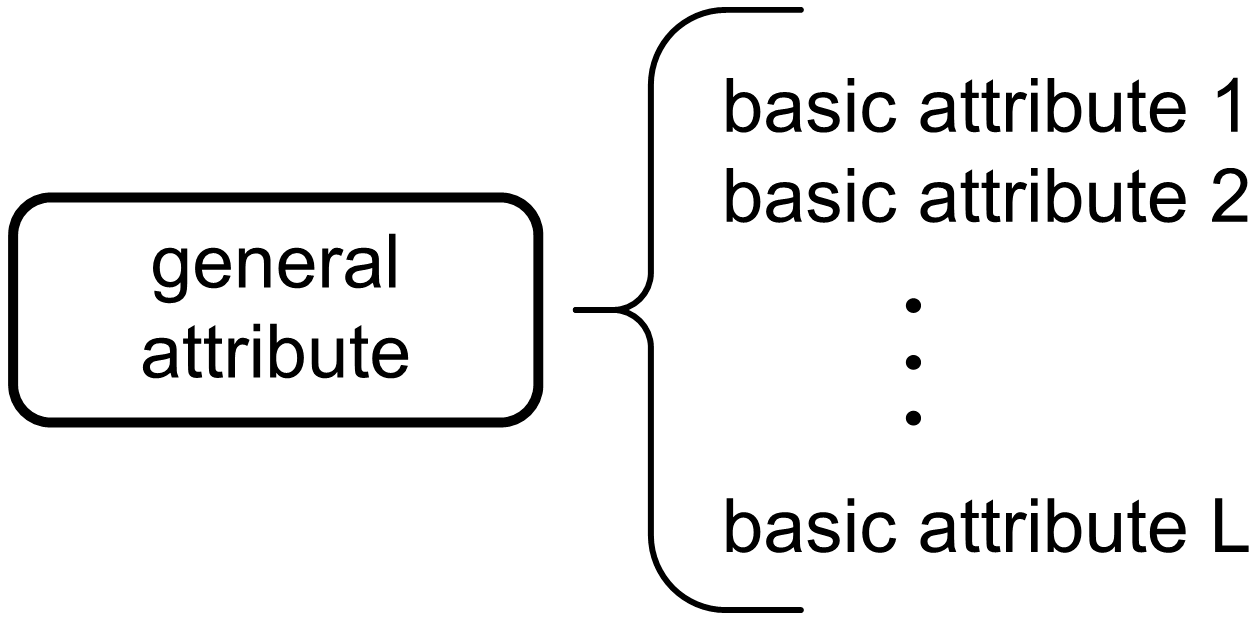
Let us assume that the ratings of the condition of the technical system can be as follows: poor, sufficient, average good, very good and excellent. The above ratings correspond to the usual numerical ratings from 1 to 5. To successfully evaluate the condition of a technical system, it is necessary to establish some hierarchy among the attributes or parts of the system. Consider an example of a hierarchical system as shown in Figure 3. It can be seen that the higher-level attributes are rated using the corresponding lower-level attributes. The attributes at the lowest level are called baseline attributes and their higher-level counterparts are the so-called general attributes. There can be any number of hierarchy levels. If the influence of an attribute cannot be determined, a reasonable degree of uncertainty can be left in the attribute evaluation process and thus, the entire system. For example, when evaluating the condition of transformer oil, the evaluator may be:

• forty percent sure that the gas concentration in the oil is at an average level and 50% sure that the gas concentration is at a very good level;
• completely confident in the assessment that the level of moisture in the oil is very good;
• fifty percent sure that the age level of the oil is at an average level and 50% sure that it is at a very good level.

In the above-mentioned estimates, the percentage ratios 40%, 50% and 100% are confidence ratings (degrees of belief) in the correctness of the given estimate and they can also be written in a decimal form as 0.4, 0.5 and 1, respectively.

It should be noted that the evaluation of the first attribute is incomplete, that is, the total sum of the confidence ratings or degrees of belief is 0.9, while in the other two cases, the evaluations are complete (moisture degree and oil age). The difference missing in the evaluation of the first attribute represents the degree of uncertainty, i.e., the uncertainty in the evaluation, so the insufficient knowledge of the baseline attributes affects the observed general attribute.

3.2. System Condition Assessment

The problem faced is to represent the overall assessment of the condition of the attribute correctly, in the case of transformer oil, considering all three baseline attributes mentioned. The following chapter will describe the original model of the proof algorithm based on the Dempster–Shafer theory [22,32,35,36], followed by the development and improvement of the baseline algorithm using the Yang–Xu axioms [34,37].

Assuming a simple two-level attribute hierarchy, a general property or a baseline attribute is at the top level and more baseline attributes are at a lower one. The organization of attributes is shown in Figure 4.

It can be assumed that there are L baseline attributes e_i (i = 1, …L) and that they are all connected with general attribute Y. In this case, it is possible to define a set of baseline attributes

E = {e₁, …e_i… e_L}.

(3)

It can also be assumed that the attribute weights are represented by ω = {ω₁, …ω_i, …ω_L} where ω_i represents the relative weight of the i-th baseline attribute e_i with a value between 0 and 1 (0 ≤ ω_i ≤ 1).

Attribute weights are important for evaluating the condition of equipment and they can be rated using different methods. To evaluate the condition of an attribute, it is necessary to define a set of possible condition evaluations. Let us assume that the ratings are represented by the following set:

H = {H₁, …H_n, …H_N},

(4)

where it is assumed that the evaluation H_n+1 is higher, i.e., it represents a better condition than H_n, therefore, set H represents an ordered set of elements, starting with the element with the lowest to the one with the highest value. Thus, the evaluation of this element of the set of baseline attributes can be determined with the following:

S(e_i) = {(H_n, β_n,i), n = 1,…N} i = 1,…, L;

(5)

where β_n,i represents the confidence rating where β_n,i ≥ 0, ${\displaystyle \sum }_{n=1}^N{\beta }_{n,i}\le 1$. If ${\displaystyle \sum }_{n=1}^N{\beta }_{n,i}=1$, then the condition assessment S(e_i) is considered complete. Otherwise, if ${\displaystyle \sum }_{n=1}^N{\beta }_{n,i}<1$, then the condition assessment of the given object S(e_i) is considered incomplete.

A special case is given by the following equation:

$${\displaystyle \sum }_{\mathrm{n}=1}^N{\beta }_{\mathrm{n},\mathrm{i}}=0$$

(6)

which indicates the complete absence of information about attribute e_i. The partial or complete absence of information about a particular attribute required for decision making is not an uncommon phenomenon. In this case, how incomplete information is handled is very important.

Let H_n be an evaluation rating and β_n the confidence rating (degree of belief in rating H_n). In this case, it is necessary to calculate the ratings H_n, confidence rating β_n of the general attributes, so that the condition estimates of all the corresponding baseline attributes e_i are considered. The process of calculating the rating and confidence ratings for a general attribute based on information related to baseline attributes is called the aggregation process. For this purpose, the following algorithm is used.

Let m_n,i be a baseline attribute weight probability, i.e. value which represents the degree of which the i-th baseline attribute e_i supports the judgment that the baseline attribute y can be estimated by a predefined rating H_n. Furthermore, we can assume that m_H,i represents the remainder of the weight probability, i.e., unassigned probability given all assigned ratings N for the given attribute e_i. The calculation of the weighted probabilities is given by the following:

m_n,i = ω_iβ_n,i    n = 1,…, N;

(7)

where ω_i represents the value resulting from the normalization of the weights of the baseline attributes. The process of normalizing the weights of the base attributes is described in the next section. The remainder of the weighting probability is calculated according to the following:

$$m_{H.i}=1-{\displaystyle \sum }_{\mathrm{n}=1}^N{m}_{\mathrm{n},\mathrm{i}}=1-{\omega }_i{\displaystyle \sum }_{\mathrm{n}=1}^N{\beta }_{\mathrm{n},\mathrm{i}}$$

(8)

It is assumed that E_I(i) represents the subset of the first i attributes E_I(i) = {e₁,e₂,…, e_i} and the weight probability m_n,I(i) is consequently defined as a rating in which all i attributes support the judgment of the attribute y being estimated at H_n. Furthermore, m_H,I(i) represents the remainder of the weight probability that is unassigned after all the baseline attributes of E_I(i) have been estimated. The weight probabilities m_n,I(i), m_H,I(i) can be calculated for E_I(i) from the basic weight probability m_n,j and m_H,j for every n = 1,…, N, and j = 1,…, i. Considering all the above facts, the original recursive algorithm of evidence-based inference can be presented using the following:

$$m_{\mathrm{n},\mathrm{I}\left(\mathrm{i}+1\right)}{=\mathrm{K}}_{I\left(\mathrm{i}+1\right)}\left(m_{\mathrm{n},I\left(i\right)}{m}_{\mathrm{n},\mathrm{i}+1}{+m}_{\mathrm{n},I\left(i\right)}{m}_{\mathrm{H},\mathrm{i}+1}{+m}_{\mathrm{H},I\left(i\right)}{m}_{\mathrm{n},\mathrm{i}+1}\right)n=1,...,N$$

(9)

$$m_{\mathrm{H},\mathrm{I}\left(\mathrm{i}+1\right)}{=\mathrm{K}}_{I\left(\mathrm{i}+1\right)}{m}_{\mathrm{H},I\left(i\right)}{m}_{\mathrm{H},\mathrm{i}+1}$$

(10)

$$K_{I\left(\mathrm{i}+1\right)}={\left[1-{\displaystyle \sum }_{t=1}^N{\displaystyle \sum }_{\begin{array}{c}j=1\\ j\ne t\end{array}}^N{m}_{t,I\left(i\right)}{m}_{j,i+1}\right]}^{-1}i=1,...,L-1$$

(11)

where K_I(i+1) represents the normalizing coefficient where the condition given by the following equation ${\displaystyle \sum }_{n=1}^N{m}_{n,I\left(i+1\right)}+m_{H,I\left(i+1\right)}=1$ is fulfilled. It is important to point out that the baseline attributes E_I(i) are arbitrarily arranged and that their initial values amount to m_n,I(1) = m_n,1 and m_H,I(1) = m_H,1. Finally, in the original proof algorithm, the combined degree of confidence for the general attribute β_n is given by the following:

$${\beta }_n{=m}_{\mathrm{n},\mathrm{I}\left(L\right)},n=1,...,N$$

(12)

$${\beta }_H{=m}_{\mathrm{H},\mathrm{I}\left(L\right)}=1-{\displaystyle \sum }_{\mathrm{n}=1}^N{\beta }_n$$

(13)

where β_H represents the degree of uncertainty or degree of estimation incompleteness.

3.3. Improved Evidential Reasoning Algorithm

The improved evidential reasoning algorithm extends the baseline algorithm and adds axioms for synthesis, which are necessary for objective and meaningful proof.

3.3.1. Baseline evidential reasoning algorithm upgrade

For the aggregation process to be objective and meaningful, it is necessary to define certain axioms for synthesis. The following axioms for the synthesis of the aggregation process were presented by Young and Xu in [37].

Axiom 1: general attribute y cannot be evaluated by H_n if none of the baseline attributes of set E is rated as H_n. This axiom is also referred to as the independence axiom. It refers to the instance, if β_n,i = 0 for every i = 1,…, L, then β_n = 0.

Axiom 2: general attribute y should be accurately graded by H_n if all baseline attributes of set E are also accurately graded by H_n. This axiom is also referred to as the consensus axiom. It refers to the instance, if β_k,i = 1 and β_n,i = 0 for every I = 1,…, L and n = 1,…, N, n ≠ k, then β_k = 1 i β_n = 0 (n = 1,… N, n ≠ k).

Axiom 3: if each baseline attribute of set e has been fully graded by a specific set of grades, then general attribute y should also be graded by the same subset of grades. This axiom is also referred to as the completeness axiom.

Axiom 4: if the evaluation of some baseline attribute of set E is incomplete to a certain degree, general attribute y will also be graded as incomplete. This axiom is also referred to as the incompleteness axiom.

It is possible to show that the original evidential reasoning algorithm does not fully satisfy the aforementioned axioms [22,34,35,36]. To ensure their fulfillment, a new or improved evidential reasoning algorithm has been presented [37]. The new approach of the method should satisfy the aforementioned synthesis axioms and provide reliable aggregation of complete and incomplete information using the new weight normalization represented by the following equation:

$${\displaystyle \sum }_{\mathrm{i}=1}^L{\omega }_i=1$$

(14)

which satisfies the consensus axiom. With the new evidential reasoning algorithm, the remainder of the weighted probability is treated separately in terms of the relative weights of the attributes and the incompleteness of the assessment. The concept of measuring the confidence rating and reliability in the Dempster–Shafer [22] inference theory can be used to select upper and lower values of the confidence rating. The improved evidential reasoning algorithm m_H,i, shown in (14), is divided into two parts:

$${\overline{m}}_{\mathrm{H},\mathrm{i}}=1-\omega$$

(15)

$${\tilde{m}}_{\mathrm{h},\mathrm{i}}{=\mathsf{\omega }}_i\left(1-{\displaystyle \sum }_{\mathrm{i}=1}^N{\beta }_{\mathrm{n},\mathrm{i}}\right)$$

(16)

with the following being true:

$${\overline{m}}_{\mathrm{H},i}+{\tilde{m}}_{\mathrm{H},i}=m_{\mathrm{H},i}$$

(17)

The first part of algorithm ${\overline{m}}_{H,i}$ represents a linear function of ${\omega }_i$ and depends on the weight of the i-th attribute. If the weight of basic attribute e_i is zero or ${\omega }_i$ = 0, ${\overline{m}}_{H,i}$ has a value of 1. Otherwise, if baseline attribute e_i dominates the assessment or ${\omega }_i$ = 1, then ${\overline{m}}_{H,i}$ has a value of 0. In simpler terms, ${\overline{m}}_{H,i}$ represents the degree of which other attributes take part in the general assessment.

The other part of the weight probability that is not assigned to any grade is ${\tilde{m}}_{H,i}$ and it is a consequence of the incompleteness of the basic attribute assessment S(e_i). If the assessment of the baseline attribute S(e_i) is complete, then ${\tilde{m}}_{H,i}$ has a value of 0, otherwise, if S(e_i) is incomplete, ${\tilde{m}}_{H,i}$ has a value proportional to ${\omega }_i$ and will be between 0 and 1.

Assuming that $m_{n,I\left(i\right)}\left(n=1,\dots ,N\right)$, ${\tilde{m}}_{H,i}$ and ${\overline{m}}_{H,I\left(i\right)}$ represent the combined weight probabilities derived from the first i assessments, the new improved algorithm can be shown as a recursion, which for (i + 1) takes into account the first i assessments, with the following:

$$m_{\mathrm{n},I\left(\mathrm{i}+1\right)}{=\mathrm{K}}_{I\left(\mathrm{i}+1\right)}\left[m_{\mathrm{n},I\left(i\right)}{m}_{\mathrm{n},\mathrm{i}+1}{+m}_{\mathrm{H},I\left(i\right)}{m}_{\mathrm{n},\mathrm{i}+1}{+m}_{\mathrm{n},I\left(i\right)}{m}_{\mathrm{H},\mathrm{i}+1}\right]$$

(18)

$$m_{\mathrm{H},I\left(i\right)}={\tilde{m}}_{\mathrm{H},I\left(i\right)}+{\overline{m}}_{\mathrm{H},I\left(i\right)}$$

(19)

$${\tilde{m}}_{\mathrm{H},I\left(\mathrm{i}+1\right)}{=\mathrm{K}}_{I\left(\mathrm{i}+1\right)}\left[{\tilde{m}}_{\mathrm{H},I\left(i\right)}{\tilde{m}}_{\mathrm{H},\mathrm{i}+1}+{\overline{m}}_{\mathrm{H},I\left(i\right)}{\tilde{m}}_{\mathrm{H},\mathrm{i}+1}+{\tilde{m}}_{\mathrm{H},I\left(i\right)}{\overline{m}}_{\mathrm{H},\mathrm{i}+1}\right]$$

(20)

$${\overline{m}}_{\mathrm{H},I\left(\mathrm{i}+1\right)}{=\mathrm{K}}_{I\left(\mathrm{i}+1\right)}\left[{\overline{m}}_{\mathrm{H},I\left(i\right)}{\overline{m}}_{\mathrm{H},\mathrm{i}+1}\right]$$

(21)

$$K_{I\left(\mathrm{i}+1\right)}={\left[1-{\displaystyle \sum }_{t=1}^N{\displaystyle \sum }_{\begin{array}{c}j=1\\ j\ne t\end{array}}^N{m}_{t,I\left(i\right)}{m}_{j,i+1}\right]}^{-1}i=1,...,L-1$$

(22)

After all L assessments have been completed, the combined confidence rating can be computed with the normalization process given with the following:

$${\beta }_n=\frac{m_{\mathrm{n},I\left(L\right)}}{1-{\overline{m}}_{\mathrm{H},I\left(L\right)}}n=1,...N$$

(23)

$$\beta =\frac{{\tilde{m}}_{\mathrm{H},I\left(L\right)}}{1-{\overline{m}}_{\mathrm{H},I\left(L\right)}}$$

(24)

As shown in (23) and (24), β_n represents the confidence rating for grade H_n to which it is assessed, while β_H represents the unassigned confidence rating and shows the incompleteness in the whole assessment process. It is possible to prove that the combined confidence ratings obtained in the aforementioned way satisfy all four synthesis axioms.

3.3.2. Expected Final Assessment of the Object Condition

If the assessments of the condition of objects obtained this way are not clear enough to highlight the difference in the grades of several different objects or several different conditions of the same object, the term expected final assessment is introduced, which indicates the equivalent numerical value of the individual scores obtained by the aggregation process.

Assume that u(H_n) represents the expected final assessment rating H_n, given the fact that u(H_n+1) > u(H_n) where H_n+1 represents a more desirable assessment rating than H_n. Expected final assessment rating u(H_n) can be computed using the probability assignment method or a regression model with partial scores or comparisons. If the final ratings are complete (β_H = 0), the expected final assessment rating of general attribute y can be computed using the following term:

$$u\left(y\right)={\displaystyle \sum }_{\mathrm{n}=1}^N{\beta }_{n}u\left(H_n\right)$$

(25)

The condition of the object represented by grade a has a more desirable rating than the condition of the object represented by grade b if the expected final assessment rating a is higher than b or u(y(a)) > u(y(b)). The confidence rating β_n given by (23) refers to the lower limit at which we can estimate general attribute y. The upper limit of the estimate is given by the plausibility method for H_n or rather (β_n + β_H). The rating range to which general attribute y can be assessed is given by the interval $\left[{\beta }_n,{\beta }_n+{\beta }_H\right]$. If the assessment of the observed object is complete, the interval is set to value β_n; specifically, the interval of confidence ratings depends on the unassigned degree of confidence ratings β_H. In any case, the value to which general attribute y can be assessed is found in the interval β_n to (β_n + β_H). According to the abovementioned, it is possible to define three values that unambiguously characterize the assessment of general attribute y, the largest, smallest and average values of the expected final assessment rating, which are given by the following:

$$u_{\max }\left(y\right)={\displaystyle \sum }_{\mathrm{n}=1}^{N-1}{\beta }_{n}u\left(H_n\right)+\left({\beta }_N{+\mathsf{\beta }}_H\right)u\left(H_N\right)$$

(26)

$$u_{\min }\left(y\right)=\left({\beta }_1{+\mathsf{\beta }}_H\right)u\left(H_1\right)+{\displaystyle \sum }_{\mathrm{n}=2}^N{\beta }_{n}u\left(H_n\right)$$

(27)

$$u_{\mathrm{avg}}\left(y\right)=\frac{u_{\max }\left(y\right)-u_{\min }\left(y\right)}{2}$$

(28)

If all of the assessments of the general attribute y are complete, i.e., for β_H = 0, the relation u(y) = u_max(y) = u_min(y) = u_avg(y) is true.

Comparing the assessment of two objects a_i and a_k based on their final ratings and corresponding intervals, it can be said that the rating of object a_i is more desirable than the rating of object a_k if and only if u_min(y(a_i)) > u_max(y(a_k)). Two objects have the same assessment if and only if u_min(y(a_i)) = u_max(y(a_k)). In every other case, comparing the assessments of two objects is incomplete and unreliable. In order to increase the reliability of the comparison of two or more objects, it is necessary to increase the quality of the initial estimates in such a way as to reduce the incompleteness in the attribute estimates for the object conditions a_i and a_k.

In short, the improved evidential reasoning algorithm consists of the aggregation and interpretation of information (5). Equation (14) is used when normalizing weight values, and, with the help of Equations (5) and (14)–(16), the baseline probability ratings are determined. For the attribute aggregation process, Equations from (18–22) are used. To obtain the combined confidence ratings, it is necessary to use Equations (23) and (24). Finally, to be able to compare the condition of two or more objects, Equations from (26–28) are used.

The next chapter presents possible methods for processing and interpreting the collected information about the condition of the system followed by a presentation of the decomposition model and assessment of the condition of the power transformer.

3.4. Input Data Analysis

Before presenting the improved evidential reasoning algorithm on a concrete example of assessing the condition of the technical system, it is necessary to further elaborate on the method of the aggregation process input data preparation, specifically, the process of analysis, processing and interpretation of data obtained by measuring or directly assessing. For such data to be used, they must be appropriately processed and transformed, usually from the quantitative to the qualitative domain, so that they satisfy Equations (4) and (5) that define the input to the aggregation process [1,2,37,38,39]. The methods used depend on the type of information and the assessor’s knowledge of the technical system. Three basic methods are presented, although it should be noted that the choice of methods and the formation of grades according to Equation (5) largely depend on the technical system itself, its nature and purpose, i.e., the method of grade formation may differ from one technical branch to another (e.g., chemical and food industry or power generation).

3.4.1. Continuous Variable as Input Data

Suppose we evaluate the condition of a system component by measuring the quantity x, which can take continuous values (e.g., breaker switch-on time, the moisture content in the transformer oil, etc.). Due to various factors in the measurement procedure, several successive measurements differ from each other. The measurement results behave according to their inherent statistical distribution. For most technical systems, the distribution is approximated by a normal or Gaussian distribution with the parameters ${\overline{X}}_i$ σ² (mean value and standard deviation). The question as to how to transform the measured value into a qualitative assessment arises [1].

According to the manufacturer’s recommendation and the user’s experience, the observed components can be classified into good or bad, i.e., classes to which we can add qualitative ratings. The classes are defined by ranges of measured size. Of course, the boundaries between classes cannot be precisely defined, so ratings will inevitably overlap. Instead of defining fixed interval boundaries, the mean and variance of the measured value are determined for each class individually.

Therefore, each class n = 1, … N is given rating H_n, mean value ${\overline{X}}_n$ and standard deviation ${\sigma }_n^2$. Parameters ${\overline{X}}_n$ and ${\sigma }_n^2$ are estimated differently depending on the type of measured quantity, type of device, manufacturer’s recommendation, fault statistics and the experience of the assessor.

To measured value x, qualitative rating H_n, with a certain degree of belief β_n is added. The degree of belief β_n is defined by the Gaussian distribution with parameters ${\overline{X}}_n$ i ${\sigma }_n^2$:

$${\beta }_n{~\mathrm{b}}_n=\frac{1}{{\sigma }_n\sqrt{2\pi }}{e}^{-\frac{{\left(x-{\overline{x}}_n\right)}^2}{2{\sigma }_n^2}}$$

(29)

It is reasonable to assume that the measurement of physical quantities is an exact procedure and that there is no indeterminacy of the results. Therefore, the sum of all probabilities β_n is unified to a value of 1:

$${\displaystyle \sum }_{\mathrm{n}=1}^N{\beta }_n=1$$

(30)

$${\beta }_n=\frac{b_n}{{{\displaystyle \sum }}_{\mathrm{n}=1}^N{b}_n}$$

(31)

The normal distribution assumes a certain probability for each measured value, so each rating would also have a certain probability. For the sake of simplicity, ratings where the probability is lower than a certain value (e.g., 0.05) can be ignored.

For attributes where the deviation from a certain ideal value is measured, which can be both positive and negative, the qualitative assessment is proportional to the absolute value of the difference between the ideal and the measured value.

The ideal trip delay time of the other two poles after the first one is t₀ = 7 ms. The maximal deviation time for a pole is Δt = 2 ms. The variable that is observed and evaluated is therefore the absolute value of measured time t and ideal time t₀:

$$\mathsf{\Delta }\mathrm{t}=\left|\mathrm{t}-{\mathrm{t}}_0\right|$$

(32)

3.4.2. Exploitation Time as Input Data

When evaluating a system component based on its age, it can start from the reliability function over time R(t). To determine the value of this function, it is necessary to know the fault statistics of such a or a similar component. A characteristic parameter is the intensity of the fault λ(t), i.e., the probability that the component will malfunction at a given point in time t. The reliability function can be described by an exponential function of time and fault intensity.

$$R\left(t\right){=\mathrm{e}}^{-{{\displaystyle \int }}_0^t\lambda \mathrm{dt}}$$

(33)

In practice, the intensity of the fault is constant during most of the exploitation time of the component and is often expressed as the mean time to failure (MTTF):

$$\mathrm{MTTF}=\frac{1}{\lambda }$$

(34)

If λ is constant, the reliability function simplifies to

$$R\left(t\right){=\mathrm{e}}^{-\mathsf{\lambda }\mathrm{t}}$$

(35)

The reliability interval $R\left(t\right)\in \left[0,1\right]$ can be split into N intervals which can be assigned qualitative ratings H_n, n = 1, …, N.

The mean value of each class R_n is transcribed to the time axis:

$$R_n{=\mathrm{e}}^{-{\mathsf{\lambda }\mathrm{t}}_n}$$

(36)

$$t_n=-\frac{1}{\lambda }\ln R_n$$

(37)

For a known component age t, qualitative grade H_n is added. The confidence rating is higher as time t approaches the middle of interval t_n. Consequently, each interval n = 1, …, N is associated with a normal distribution with expectancy μ_n = t_n:

$${\mathrm{b}}_n=\frac{1}{{\sigma }_n\sqrt{2\pi }}{e}^{-\frac{{\left(t-{\mathrm{t}}_n\right)}^2}{2{\sigma }_n^2}}$$

(38)

Standard deviation σ_n is chosen so that the following conditions are met:

$$b_n\left(t_n\right){=\mathrm{R}}_n$$

(39)

$${\sigma }_n=\frac{1}{R_n\sqrt{2\pi }}$$

(40)

As with the previous method, the overall confidence rating is normalized according to the equation:

$${\beta }_n=\frac{b_n}{{{\displaystyle \sum }}_{\mathrm{n}=1}^N{b}_n}\cdot \left(1-{\beta }_H\right)$$

(41)

where β_H represents the measurement ambiguity, which can arise as a consequence of disregarding certain factors such as specific component age or the exact amount of malfunction occurrence on such devices.

3.4.3. Discrete Variable as Input Data

Generally speaking, discrete variable x can retain a finite number of values K:

$$x\in \left\{x_k;k=1,2,...,K\right\}$$

(42)

assuming x_k being:

• a specific numerical value (e.g., number of surge arrester operations);
• one of the conditions from a finite set of possible conditions (e.g., condition of a Buchholz relay: A—normal, B—warning and C—trip);
• a descriptive value (e.g., good, bad, average).

In most cases, the number of values K is not large, i.e., it generally does not exceed 10. For a larger number of values, the previously mentioned methods for continuous variables can be used.

Each value x_k is associated with the set of qualitative grades with the corresponding confidence ratings:

$$x\in \left\{x_k;k=1,2,...,K\right\}$$

(43)

The most straightforward way of grade assignment is creating a lookup table.

Table 1. Transformation table for converting discrete conditions into qualitative ratings.

Condition\ Grade	H1	H2	…	Hn		HN
x1	β11	β21	…	βn1	…	βN1
x2	β12	β22	…	βn2	…	βN2
…	…	…		…		…
xk	β1k	β2k		βnk	…	βNk
…	…	…		…		…
xK	β1K	β2K	…	βnK	…	βNK

presents a method for converting discrete conditions into qualitative ratings.

In practice, each condition is generally assigned only one or two grades, so most table elements will be equal to zero. The degree of uncertainty of each condition is calculated from the sum of the confidence ratings for one condition:

$${\beta }_{\mathrm{Hk}}=1-{\displaystyle \sum }_{\mathrm{n}=1}^N{\beta }_{\mathrm{nk}}$$

(44)

Coefficients β_nk for a specific type of system component is determined by the expert assessor or a group of them. Determination methods are mainly based on empirical rules that are defined for each case separately.

Different types of data require different techniques and approaches to the transformation process, where the practical experience and knowledge of experts can be of a significant value [2,23]. Only when the information about the baseline attributes of one or more observed objects has been collected and represented suitably can the evaluation of the condition of general attributes and, finally, the evaluation of the condition of the whole object or system be initiated.

3.5. Decomposition Model and Transformer Condition Assessment

In order to assess the condition of a complex technical system, such as a power transformer, it is necessary to collect, process and interpret a large amount of qualitative and quantitative information [2,7,15,23,25,35,40]. The required information is obtained by measuring and evaluating the observed object itself or by using remote monitoring and continuous information gathering. Regardless of the way the information is collected, it is necessary to transfer it to the qualitative domain using the appropriate semantic apparatus and the methods described in the previous chapter. Let us assume that the information has been successfully collected and transferred to the appropriate qualitative domain, that the attributes from Equation(3) have been successfully evaluated with the set of ratings defined by Equation (4) and that the attribute ratings have been given according to Equation (5).

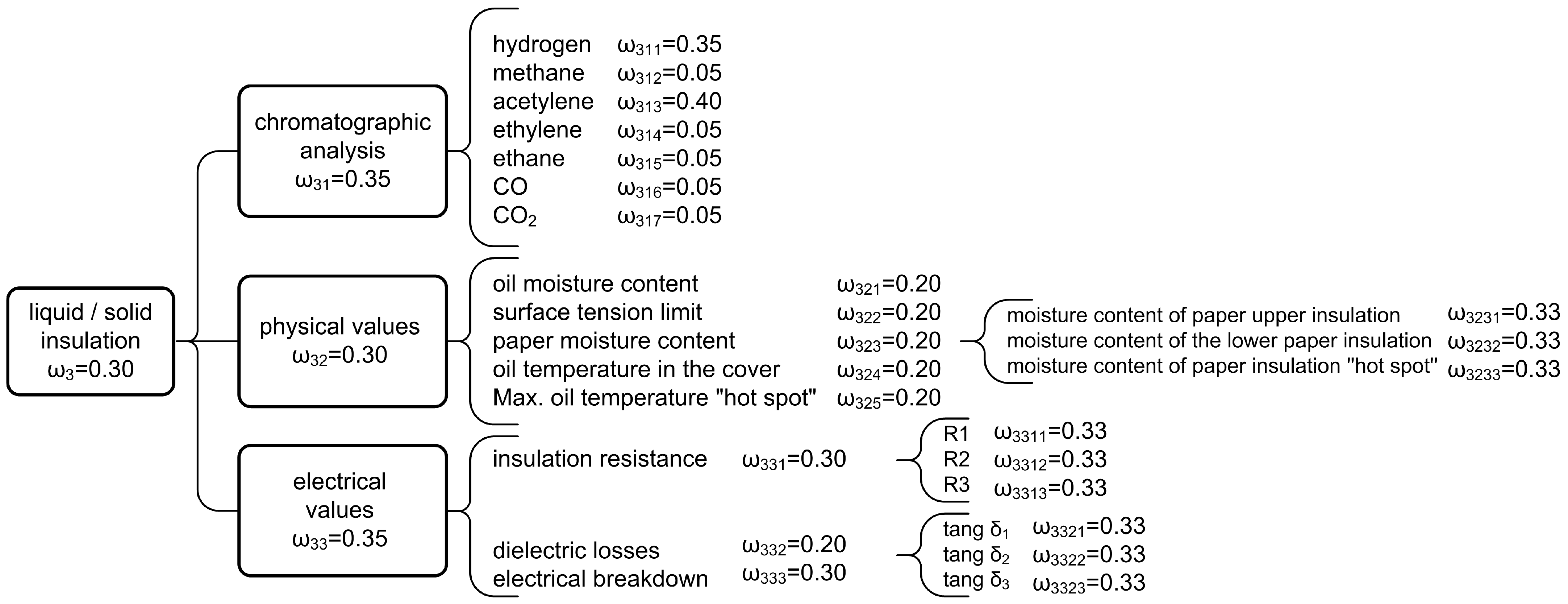
Considering all of the above, a general attribute or property based on the attributes directly or via lower-order attributes can be estimated depending on the used decomposition model. For instance, the condition of liquid or solid insulation of a power transformer can be determined by a chromatographic analysis and by measuring physical and electrical parameters. Chromatographic analysis determines the percentage of characteristic gases dissolved in oil (hydrogen, methane, acetylene, ethylene, etc.), the measurement of physical parameters determines the oil moisture, paper insulation, borderline surface tension, oil temperature, etc., while the measurement of electrical parameters determines insulation resistance, dielectric loss factor, oil dielectric strength and other quantities, as shown in Figure 4, Figure 5 and Figure 6, with Figure 5 showing a multi-stage decomposition model for a power transformer. Figure 6 shows the decomposition of a second-level attribute, i.e., it shows the decomposition of liquid rigid insulation. In the decomposition from general to baseline attributes, several levels of attributes can be seen. Each attribute e_i from a set of baseline attributes E should have a defined weight ω_i and a confidence rating βi regarding the grade H_n.

For the purpose of this paper, a power transform [18,41,42,43,44] has been chosen as a proof of concept (PoC) example for a technical system and a decomposition model has been created for the same, with the corresponding general and baseline attributes. All attributes e_i of the given model have been assigned their appropriate weights ω_i. For the baseline attributes, values for which appropriate measurements can be carried out or be estimated for which confidence rating βi can be determined to its respectable grade H_n. Since this is an extremely complex technical system consisting of several subsystems, determining the decomposition model is not a simple task. By creating a decomposition model, an attempt was made to decompose the power transformer into as many independent baseline elements of the system as possible, the condition of which can be determined by measurement or evaluation. The system elements in the decomposition model are called system attributes (3), and in the following text, the term system attribute will refer to the element of the decomposed system.

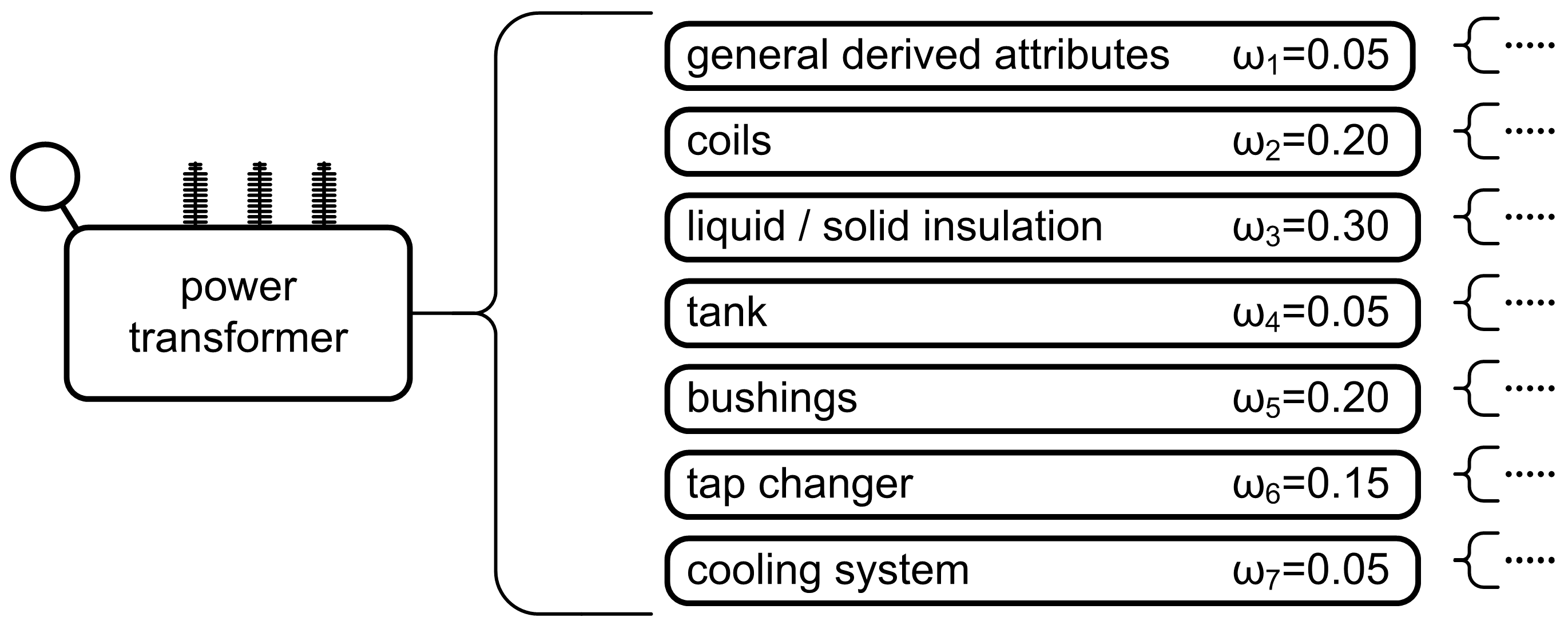
Figure 5 shows the proposed power transformer decomposition model. There is a clear split into seven general attributes, which represent certain parts of the observed technical system and give an insight into the generally derived attributes, winding condition, liquid or solid insulation condition, boiler condition, conductor condition, control cover condition and cooling system condition. Each of the listed seven general attributes is divided into lower-order attributes down to the baseline attributes. For example, the condition of the winding is represented by four general attributes, i.e., condition of the winding capacitance, magnetizing current, active resistance of the winding and control of the winding displacement. Each of the four listed general attributes are represented by a certain number of baseline attributes. For example, in the case of winding capacitance, the baseline attributes are three measurable values expressed in pF, i.e., C1, C2 and C3, representing the winding capacity measured at different measuring connections. A similar division can be seen for all other attributes.

3.5.1. Baseline Attributes

The overall decomposition model consists of five levels, as shown in Figure 5 and Figure 6. At the first and baseline stage, the overall condition of the observed object, i.e., the power transformer, is represented; at the second level, seven general attributes provide information about the general condition, the condition of the winding, liquid or solid insulation, boiler, conductor, switchgear and the cooling system. On the third level, there are general attributes, which represent more elaborated general attributes of the second level and a certain number of baseline attributes. The fourth level contains mainly baseline attributes and a smaller number of general attributes represented by their baseline attributes on the fifth level. In short, the proposed model consists of 91 baseline attributes whose data from the remote monitoring system are available, i.e., corresponding measurements can be made or condition assessments performed.

Table 2. Proposed baseline attributes of a power transformer decomposition model.

# 1	Baseline Attribute Type	Description	Unit	Collection Means	Weight
1.	Load			Type 2	${\omega }_{11}=0.33$
2.	Remaining life span		year	Type 2	${\omega }_{12}=0.33$
3.	Aging momentum			Type 2	${\omega }_{13}=0.33$
4.	C1 ((HV+MV):STN)	Winding capacity in the measured connection (HV + MV):STN	pF	Type 1	${\omega }_{211}=0.10$
7.	I1 (HV Phase U)	Magnetizing current for HV Phase U	mA	Type 1	${\omega }_{221}=0.166$
13.	R1 (HV: 1U-N)	Winding active resistance between HV: 1U-N	R/Ω	Type 1	${\omega }_{231}=0.143$
20.	Asymmetry Lx1	Dissipative inductance of winding pairs with tap changer position being 1	%	Type 1	${\omega }_{241}=0.33$
23.	Hydrogen	Gases dissolved in transformer oil concentration	μL/L (ppm)	Type 1/2	${\omega }_{311}=0.40$
24.	Methane	Gases dissolved in transformer oil concentration	μL/L (ppm)	Type 1/2	${\omega }_{314}=0.05$
25.	Acetylene	Gases dissolved in transformer oil concentration	μL/L (ppm)	Type 1/2	${\omega }_{313}=0.40$
26.	Ethylene	Gases dissolved in transformer oil concentration	μl/L (ppm)	Type 1/2	${\omega }_{314}=0.05$
27.	Ethane	Gases dissolved in transformer oil concentration	μL/L (ppm)	Type 1/2	${\omega }_{315}=0.05$
28.	Carbon monoxide	Gases dissolved in transformer oil concentration	μL/L (ppm)	Type 1/2	${\omega }_{316}=0.05$
29.	Carbon dioxide	Gases dissolved in transformer oil concentration	μL/L (ppm)	Type 1/2	${\omega }_{317}=0.05$
30.	Oil moisture	Gases dissolved in transformer oil concentration	mg/kg	Type 1/2	${\omega }_{321}=0.20$
31.	Borderline surface tension	Borderline surface tension at 20 °C	mN/m	Type 1	${\omega }_{322}=0.20$
32.	Paper moisture		%	Type 2	${\omega }_{323}=0.20$
35.	Oil temperature in the boiler cover		°C	Type 2	${\omega }_{324}=0.20$
36.	Hot-spot oil temperature		°C	Type 2	${\omega }_{325}=0.20$
37.	R1 ((HV + MV):STN)	Insulation resistance of the winding and the core between (HV + MV):STN	GΩ (10min)	Type 1	${\omega }_{3311}=0.33$
40.	tan δ1 ((HV + MV):STN)	Winding insulation Dielectric loss factor between (HV + MV):STN	%	Type 1	${\omega }_{3321}=0.33$
43.	Oil dielectric strength	Physicochemical tests of transformer oil	kV	Type 1	${\omega }_{333}=0.30$
44.	Boiler air dryer			Type 1	${\omega }_{41}=0.33$
45.	Boiler oil level			Type 1	${\omega }_{42}=0.33$
46.	Seal loosening			Type 1	${\omega }_{43}=0.33$
47.	tan δ1 (N)	Conductor dielectric loss factor (N)	%	Type 1	${\omega }_{511}=0.143$
52.	tan δ6 (2V)	Conductor dielectric loss factor (2V)	%	Type 1	${\omega }_{516}=0.143$
53.	tan δ7 (W)	Conductor dielectric loss factor (2W)	%	Type 1	${\omega }_{517}=0.143$
54.	C1 (N)	Conductor insulation capacity (Ground point)	pF	Type 1	${\omega }_{521}=0.143$
55.	C2 (1U)	Conductor insulation capacity (Phase)	pF	Type 1	${\omega }_{522}=0.143$
61.	Conductor thermal imaging			Type 2	${\omega }_{53}=0.10$
62.	Phase shift index 1U	Primary side conductor capacity change index (1U)		Type 2	${\omega }_{541}=0.33$
68.	Number of tap changer operations			Type 2	${\omega }_{61}=0.25$
69.	Total switched current		kA	Type 2	${\omega }_{62}=0.25$
70.	Tap changer motor power		%	Type 2	${\omega }_{63}=0.40$
71.	Tap changer boiler air dryer			Type 1	${\omega }_{64}=0.10$
72.	Pump 1 condition			Type 2	${\omega }_{711}=0.20$
77.	Ventilator 1 condition			Type 2	${\omega }_{721}=0.10$
87.	Cooler 1 efficiency		%	Type 2	${\omega }_{731}=0.20$
91.	Cooler 5 efficiency		%	Type 2	${\omega }_{735}=0.20$

¹ Some attributes from the same data spectrum are omitted in order to preserve space.

lists the most relevant of the baseline attributes proposed in this model with a brief description. In addition, the units of measurement and methods of data acquisition are indicated, i.e., whether the data were collected by measuring and checking the system (offline data, labeled Type 1 in Table 2) or whether they were obtained from a remote monitoring and data collection system (online data, labeled Type 2 in Table 2)

Based on the quantitative ratings collected, it is necessary to determine qualitative ratings for the above baseline attributes. The qualitative ratings of baseline attributes, together with the weights of the individual baseline attributes form the input for the aggregation process. Ratings of the baseline attributes present the basis for the ratings of the general attributes. Performing aggregation process ratings of the higher-level attributes are determined. By repeating the aggregation process up to the highest level, the condition assessment of the entire observed object is determined. The following chapter describes the condition assessment procedure for the power transformer.

3.5.2. Condition Assessment

To assess the condition of the energy transformer, real maintenance data from the Croatian Transmission Grid Operator company are used; specifically, data regarding the energy transformer Končar, type 1 ARZ 300000-420/A. The data cover the continuous period of six years. In general, the offline (Type 1) data were collected at least once a year to a maximum of four times a year and basically at irregular intervals, although for a certain subset of data, there were regular intervals between the collected data.

For the first four years, data were obtained by measurement or assessment (offline data) and since the beginning of the fifth year, data from the remote monitoring system (online data) are also available. Therefore, it can be said that the data collected within the observed six years vary both in the amount of collected data (the number of baseline attributes for which data are available at a given time) and in the source of the data (data collected offline and/or online).

After defining the available data by time points, it is possible to transform the existing quantitative data into a qualitative domain, i.e., to add corresponding ratings to the collected data that represent the evaluation of a certain baseline attribute. Table 2 also shows the boundary conditions for data conversion and an indication of the qualitative ratings is given for each basic attribute for which input data are available. Condition assessment of a certain general attribute begins by going over the confidence rating in grade H_n, its baseline attributes e_i, respecting their weights ω_i and performing the aggregation procedure as shown in Equations from (18–25). Condition assessment of the observed general attribute is then represented by a probability distribution, i.e., by the confidence rating in the assessments from set H_n as shown in (25). For the condition comparison of two or more points in time, the terms from (26–28) can be used.

All computations required to perform the aggregation procedure were performed numerically using the condition assessment application developed by the authors. To describe the computation procedure, the computation of the condition of the power transformer for the latest point in time is presented in abbreviated steps. The chosen example is interesting due to the largest amount of available data.

In order to successfully commence the calculation procedure, it is assumed that all available quantitative data for the basic attributes have been collected and weights have been set for all attributes, both general and baseline. According to the qualitative data presented in Table 2, the aggregation procedure starts with the baseline attributes and general attributes. Complex mathematical steps in performing the aggregation procedure are omitted here, and the procedure is presented in detail in [3,37], so only the final values of the general attribute ratings are shown.

Taking into account the confidence ratings βi in grade H_n for baseline attributes e_i and their assigned weights ω_i, and after carrying out the aggregation procedure for the second level general attributes, the following distributions are obtained:

S (Load) = {(excellent, 1)} S (Remaining life cycle) = {(excellent, 1)} S (Aging momentum) = {(excellent, 1)} S (General derived attributes) = {(excellent, 1)} S (Winding capacity) = {(excellent, 1)} S (Magnetizing current) = {(excellent, 1)} S (Winding active resistance) = {(excellent, 1)} S (Winding shift control) = {(excellent, 1)} S (Windings) = {(excellent, 1)} S (Chromatography) = {(unsatisfactory, 0.0295), (very good, 0.2489), (excellent, 0.7216)} S (Physical values) = (very good, 0.0454), (excellent, 0.08275), (H, 0.1271)} S (Electric values) = {(excellent, 0.7895), (H, 0.2105)} S (Liquid/solid isolation) = {(unsatisfactory, 0.0084), (very good, 0.0823), (excellent, 0.8306), (H, 0.0787)} S (Boiler air dryer) = {(excellent, 1)} S (Boiler oil level) = {(excellent, 1)} S (Seal loosening) = {(excellent, 1)} S (Boiler) = {(excellent, 1)} S (Conductor insulation dielectric loss factor) = {(good, 0.0563), (very good, 0.2550), (excellent, 0.6886)} S (Conductor insulation capacity) = {(excellent, 1)} S (Conductor thermal imaging) = {(H, 1)} S (Primary side capacity shift index) = {(very good, 0.2951), (excellent, 0.7409)} S (Secondary side capacity shift index) = {(very good, 0.1212), (excellent, 0.8788)} S (Conductors) = {(good, 0.0035), (very good, 0.1492), (excellent, 0.7920), (H, 0.0554)} S (Number of operations) = {(excellent, 1)} S (Total switched current) = {(excellent, 1)} S (Tap changer motor power) = {(excellent, 1)} S (Tap changer) = {(excellent, 1)} S (Pump condition) = {(excellent, 1)} S (Ventilator condition) = {(excellent, 1)} S (Cooler efficiency) = {(excellent, 0.5355), (H, 0.4645)} S (Cooling system) = {(excellent, 0.9394), (H, 0.0606)} which results with the following distribution: S (ET)Seventh/May = {(unsatisfactory, 0.0019), (good, 0.0005), (very good, 0.0385), (excellent, 0.9331), (H, 0.0261)}

which represents the overall condition assessment of the power transformer for the chosen point in time.

From the above, it can be seen that the overall condition of the power transformer is rated as unsatisfactory with a confidence rating of 0.019, good with a rating of 0.0005, very good with a rating of 0.0385 and excellent with a rating of 0.9331. The uncertainty of the assessment is 0.0261 and results from the absence and/or unfamiliarity of all defined input data.

To obtain a more comparable grade, it is possible to calculate the final assessment. For this purpose, it is first necessary to determine the intervals corresponding to the five basic grades. Suppose the values are chosen as follows:

• u (1) = 0;
• u (2) = 0.35;
• u (3) = 0.55;
• u (4) = 0.85
• u (5) = 1.

By applying (14–28) to the above distributions, the overall condition assessment of the observed object is obtained as follows:

u((ET)_Seventh/May)_min = 0.9661

(45)

u((ET)_Seventh/May)_max = 0.9921

(46)

u((ET)_Seventh/May)_avg = 0.9791

(47)

with the following being true:

u((ET)_Seventh/May) = u((ET)_Seventh/May)_avg ± Δu = 0.9791 ± 0.013

(48)

Using the final condition assessment and the interval of the final rating, a numerical value and the width of the value interval that represents the overall condition of the observed object can be determined. Such a value can be used to compare the state of different observed objects. It is also possible to represent the final condition rating as a function of time and observe the change of the condition during the period of use and the improvement of the condition rating after maintenance.

For all selected time points, the aggregation procedure was carried out, and the results are shown in

Table 3. Power transformer condition assessments at different points in time.

#	Year	Month	Rating 1	Rating 2	Rating 3	Rating 4	Rating 5	Uncertainty	Uavg	Umin	Umax
1	First	August	0.0000	0.0000	0.0331	0.0592	0.3420	0.5656	0.6934	0.4106	0.9762
2	Second	February	0.0000	0.0000	0.0304	0.0244	0.4030	0.5422	0.7116	0.4405	0.9827
3	Second	August	0.0000	0.0000	0.0586	0.0000	0.3814	0.5600	0.6936	0.4136	0.9736
4	Third	February	0.0000	0.0000	0.0665	0.0000	0.3503	0.5832	0.6785	0.3869	0.9701
5	Third	August	0.0000	0.0000	0.0486	0.0184	0.7001	0.2329	0.8589	0.7425	0.9754
6	Forth	February	0.0000	0.0000	0.0059	0.0600	0.3285	0.6056	0.6855	0.3827	0.9884
7	Forth	September	0.0000	0.0057	0.0643	0.0620	0.2727	0.5954	0.6604	0.3627	0.9581
8	Fifth	September	0.0000	0.0046	0.0000	0.0508	0.4003	0.5443	0.7172	0.4451	0.9894
9	Sixth	February	0.0000	0.0025	0.0045	0.0350	0.7651	0.1930	0.8946	0.7981	0.9911
10	Sixth	May	0.0000	0.0030	0.0000	0.0211	0.7525	0.2234	0.8832	0.7714	0.9949
11	Sixth	September	0.0000	0.0023	0.0006	0.0190	0.7843	0.1938	0.8985	0.8016	0.9954
12	Sixth	December	0.0026	0.0000	0.0027	0.0103	0.7724	0.2119	0.8886	0.7827	0.9946
13	Seventh	May	0.0019	0.0000	0.0005	0.0385	0.9331	0.0261	0.9791	0.9661	0.9922

from which the exact moments of data acquisition (time), confidence rating in the individual ratings (Rating 1, Rating 2, etc.), uncertainty and the overall condition assessment (u_avg, u_min, u_max) are clearly visible.

Table 3 shows the final assessment and the overall rating of the power transformer at different time points. The influence of incomplete input data in the aggregation process due to an increased uncertainty is also clearly visible. Due to the increased uncertainty, there is also an increased dispersion of the overall score u and to an increased interval of overall score Δu.

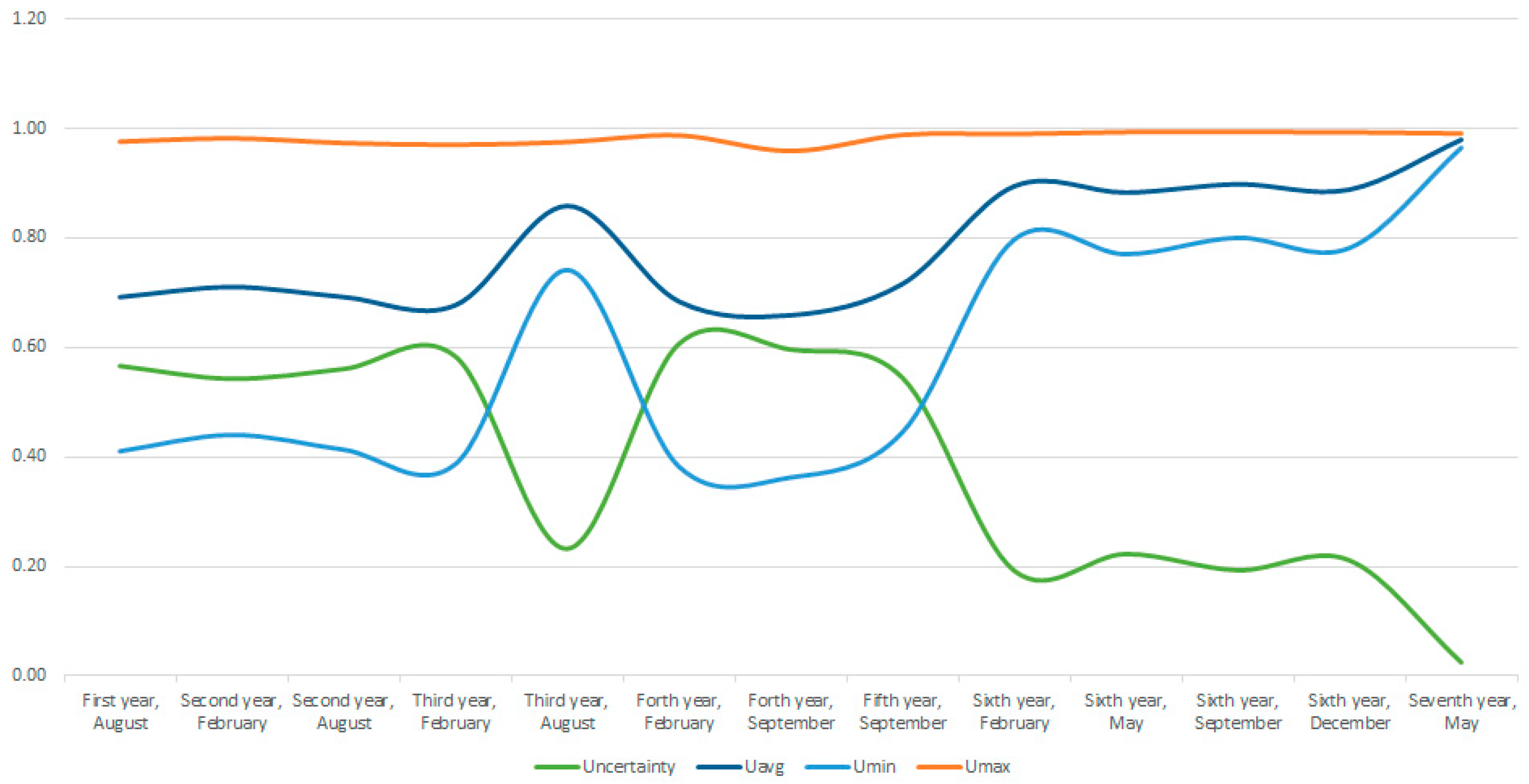
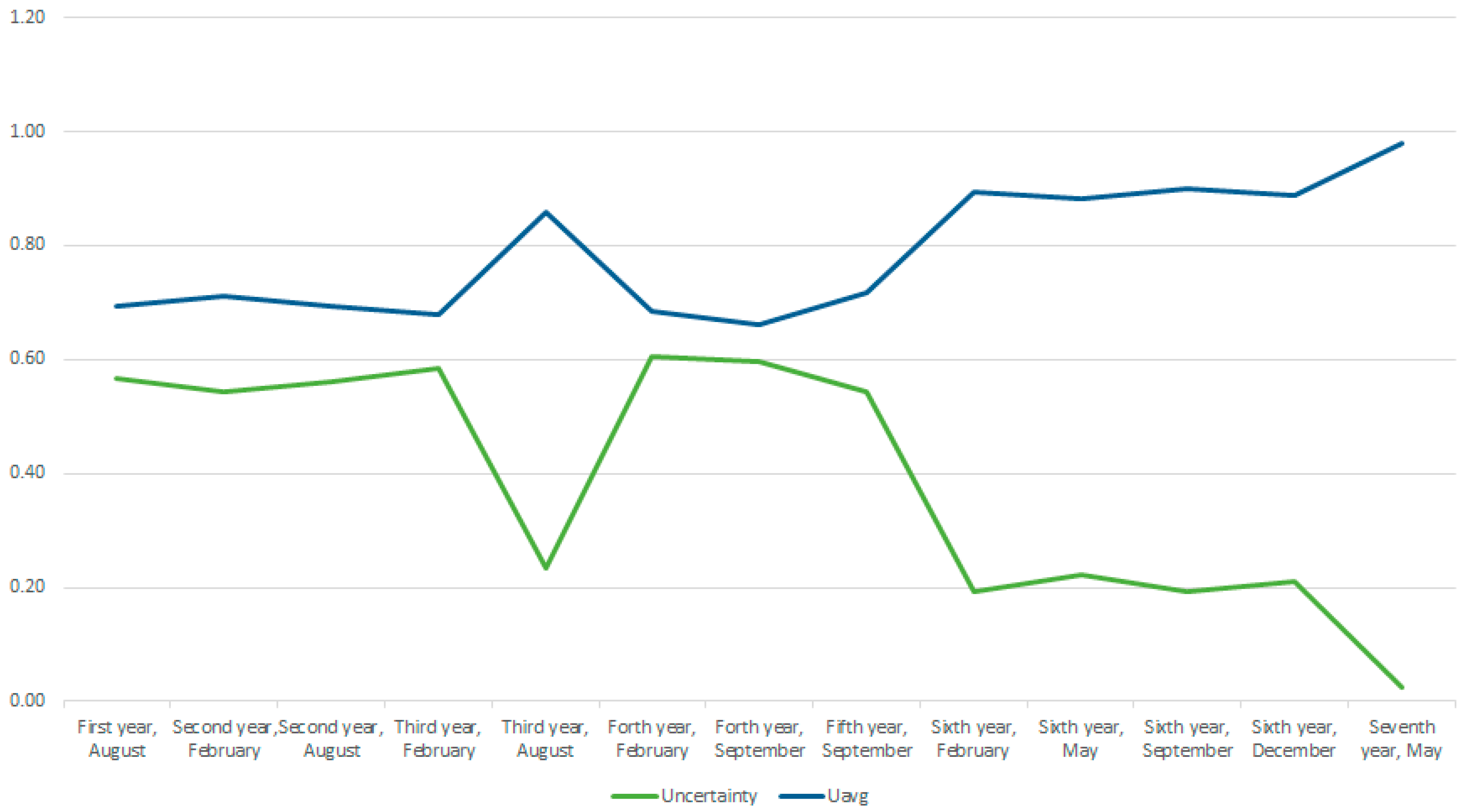
Figure 7 and Figure 8 show the relationships between the uncertainty and parameters of the overall assessment of the time of data acquisition. Therefore, Figure 7 shows the visible relationship between the uncertainty, average, minimum and maximum total score. Figure 8 shows the relationship between the uncertainty or incompleteness of the input data and the average overall score, which clearly shows that the completeness of the input data is desirable. Uncertainty, for the data collected until February of the sixth data year, ranges from 0.54 to 0.6, with the exception of August of the third data year, when, in addition to the usual measurements, measurements of electrical quantities (windings, liquid/solid insulation, conductors) were also performed.

The greatest uncertainty is present for the measurements carried out in February of the fourth data year, when, of the input data predicted by the model, only some of the values were available, measured ones (chromatography, oil moisture, thermal imaging of conductors) and inspected ones (boiler, pump conditions, ventilator conditions). Data from the remote data collection system were not available after February of the sixth data year. Since then, data from the remote monitoring system were available, which resulted in a reduction of uncertainty, and the smallest recorded uncertainty is recorded in May of the seventh data year, when almost all the data predicted by the model were available, meaning that input data obtained by measurement and assessment, and the remote monitoring data were available.

After analyzing the obtained data, based on the proposed model and the evaluation procedure, it is evident that adequate attention should be addressed to the input data, i.e., to ensure as much input data as possible. The previous procedures in the maintenance of power transformers were based on regular (periodic) or emergency measurements and tests, which results in oscillations in the amount of input data. To compare the score and two or more conditions of the observed object, it is desirable to take time points with as complete data as possible.

3.6. Analysis Results and Uncertainty Review

The observed baseline or general attributes, i.e., assessment evaluations, may be subject to some uncertainty, i.e., incomplete knowledge of the information, which negatively affects the assessment procedure itself. The degree of uncertainty depends on the amount of information, i.e., the available data, the assessor’s knowledge of the equipment and devices installed in the observed object and the possibility of a complete assessment of individual attributes. The examples clearly show that some attributes can be fully assessed with an appropriate rating, but that there is always a certain part of the information for which the occurrence of uncertainties cannot be avoided and that these uncertainties can sometimes be significant. The analysis of data collected by the system’s technical diagnostics and the linking of appropriate assessments and decisions must be performed in an objective, reliable, repeatable and transparent manner. The above conditions can be satisfied by using an improved evidential reasoning algorithm as a decision-making support tool in a multi-attribute environment [3,23,33,39]. The improved evidential reasoning algorithm satisfies all four axioms of synthesis [34,37] and allows attributes to participate in the assessment based on their weights. The example clearly demonstrates the different influences of attributes due to the difference in their weights, i.e., different individual weight ratings. In most cases, the choice of weight ratings is the result of the assessor’s knowledge of the technical system and the production process. It is important to note that the weighting coefficients and rules used to convert the rating of basic attributes are not generally accepted technical guidelines but are a proposal of the team of the authors to present the method. The weighting ratings and conversion rules should be carefully considered and selected for each observed technical system. The improved evidential reasoning algorithm is resistant to incomplete information about baseline or general attributes, which is an important property that provides an insight into the impact of incomplete knowledge of information related to the baseline attribute and the overall uncertainty in the evaluation of the entire technical system. The uncertainty of the final assessment must be within reasonable limits for the overall system assessment to be meaningful. It is also possible to display the result of the condition assessment as a single numerical value with an interval between the minimum and maximum values rather than an assessment spread over several predefined grades. Such a numerical value allows an easy insight into the state of the system and comparison of the state of the observed system with other similar systems or with the state of the same technical system at another time. Special emphasis is placed on the correct interpretation of physical quantities obtained from measurements of system parameters. It is necessary to adequately process the quantitative information collected and transfer it to the qualitative domain. This information is ranked and used as input to the aggregation process. If an error occurs at this stage, it will affect the final score depending on the individual weighting of the attribute. If the collection of information and the evaluation of the condition is done continuously or at regular time intervals, there is enough information to represent the condition of the observed object as a function of time. Based on the analysis of such a time function, it would be possible to make maintenance-related decisions. In cases where the condition of the technical system is described using a time function and an appropriate knowledge base, it is possible to predict situations that are amenable to failure. This significantly reduces the possibility of malfunctions with serious consequences for the condition of the system. The lower limit of the system condition, at which intervention is not yet required but preparation for system maintenance should be started, is evaluated as “sufficient”, i.e., when the overall system rating decreases or approaches the predefined lower value, preparations for maintenance of the components with the worst condition must be started and maintenance carried out before the system rating decreases to the unsatisfactory value, i.e., before the overall system rating falls below the permissible critically low value. Critical parts of the system can be assigned high-weight coefficients so that their possible unsatisfactory state is reflected in the overall state of the system. An example of evaluating the state of a power transformer illustrates the complexity of the computation and aggregation process. The influence of incomplete assessments of baseline attributes on general attributes and the final evaluation of the condition is presented. The influence of the weighting of individual attributes on the aggregation process becomes visible. The example illustrates the importance of a system for remote monitoring and data collection as well as supplementing the data collected in this way with data collected through measurements and regular inspections of the system. With the help of such a tool or a toolbox, it is possible to see the current condition of the object, the deterioration of the condition before and after a certain period of use and repairs or the improvement of the condition after the maintenance process. It is possible to observe how and to what extent individual maintenance actions affect the condition of the observed system and it is possible to maintain the condition of the system at a certain qualitative level by influencing the condition of various baseline attributes. Further development of the proposed model could be in the direction of improving the organization of data acquisition, placing a greater emphasis on continuous measurements and data collection, and incorporating algorithms for input data analysis, state assessment and condition prediction of the observed objects. Since most modern equipment in power plants has some degree of embedded measurement, i.e., embedded systems and diagnostic capabilities, adding such algorithms and interfacing with remote data acquisition equipment should be a feasible task.

4. Conclusions

The conducted research shows that the condition of a complex technical system can be adequately represented by a numerical value, or an ordered set of values, that represents a qualitative assessment of the system condition and that an insight into the system state can be gained on this assessment. The development of this proposed model of maintenance by condition assessment requires the previous experience of experts and maintainers, certain elements of which are incorporated into the proposed methods and procedures. The proposed model can be easily adapted to be used in plants of another technical and technological framework. The first step in the maintenance model for technical systems is to decompose the system and determine the parameters essential for the proper operation of a particular plant by evaluating its condition. Decomposition is followed by the measurement of the physical quantities, inspection and data acquisition by the installed measuring devices. The aggregation procedure is carried out based on an improved evidential reasoning algorithm, which is a way to objectively consider the weights of each baseline attribute, its influence on the general attributes, the overall assessment and the uncertainty of the input assessment itself. After the aggregation procedure, the final evaluation of the state of the observed object is obtained, which is represented as a probability distribution of all input evaluations. This type of representation is quite complex, so for mutual comparison of the condition of the observed object, the final score, represented by a numerical value, and the dispersion interval of the final score are used. The improved evidential reasoning algorithm can adequately deal with incomplete information about a baseline or general attributes. This is an important feature that provides an insight into the impact of incomplete knowledge of information related to the baseline attributes on the overall uncertainty in the evaluation of the entire technical system. The result of the condition assessment can be displayed as a single numerical value with an interval between the minimum and maximum values, rather than an assessment spread over several predefined grades. Such a numerical value allows an easy insight into the system state and the comparison of the state of the observed system with other similar systems or with the state of the same technical system at another time. Special attention must be paid to the correct interpretation of the physical quantities obtained from the measurements of the system parameters. It is necessary to adequately process the collected quantitative information and translate it into the qualitative domain. This information is ranked and used as input to the aggregation process. If the information collection and condition assessment are done continuously or at regular time intervals, sufficient information is available to represent the state of the observed object as a function of time. Based on the analysis of such a time function, it is possible to make decisions regarding maintenance. In cases where the state of the technical system is described with the help of a time function and a suitable knowledge base, it is possible to predict situations suitable for faults. This significantly reduces the possibility of malfunctions with serious consequences for the condition of the system. The lower limit of the system condition, at which intervention is not yet required but preparation for maintenance of the system should be started, is rated as “sufficient”, i.e. when the overall system rating drops or approaches the predefined lower value, preparations for maintenance of the components with the worst condition must be started and maintenance performed before the system rating drops to the unsatisfactory value, i.e. before the overall system rating drops below the allowable critical low value. Critical system components can be assigned high-weighting coefficients so that their potentially unsatisfactory condition is better reflected in the overall condition of the system. The contribution of the presented novel approach can be summarized as a proposal of a state model for power transformers suitable for maintenance purposes by evaluating the state of the objects, which can be represented as a function of time and operating conditions. The proposed model could be further developed by improving the organization of data collection, by placing more emphasis on continuous measurements and data acquisition, and by integrating algorithms for input data analysis, condition assessment and even prediction into the observed objects themselves. Since most modern equipment in power plants has embedded measurement devices and diagnostic functions, it should be a feasible task to add such algorithms and interface them with remote data acquisition equipment.