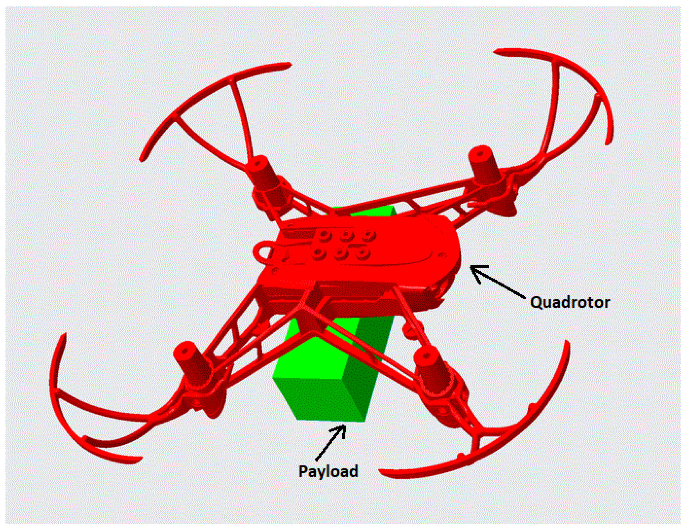
Figure 1.
The 3D CAD model of quadrotor with Payload.
Figure 1.
The 3D CAD model of quadrotor with Payload.
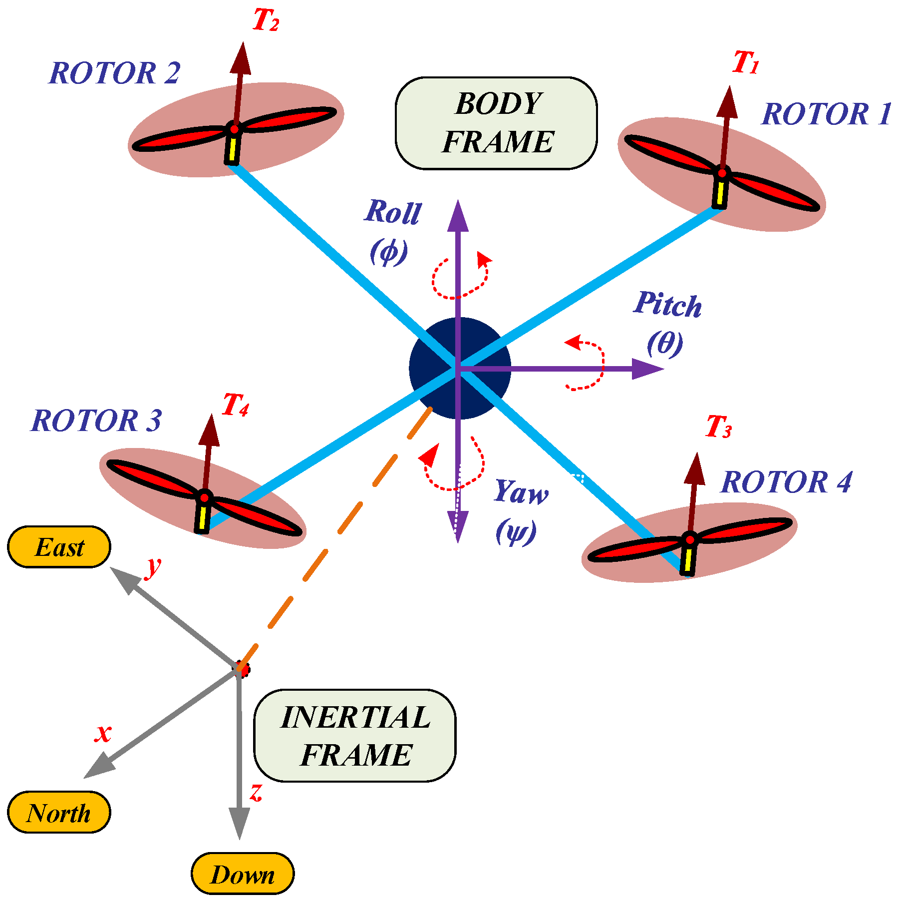
Figure 2.
The X-configuration of quadrotor.
Figure 2.
The X-configuration of quadrotor.
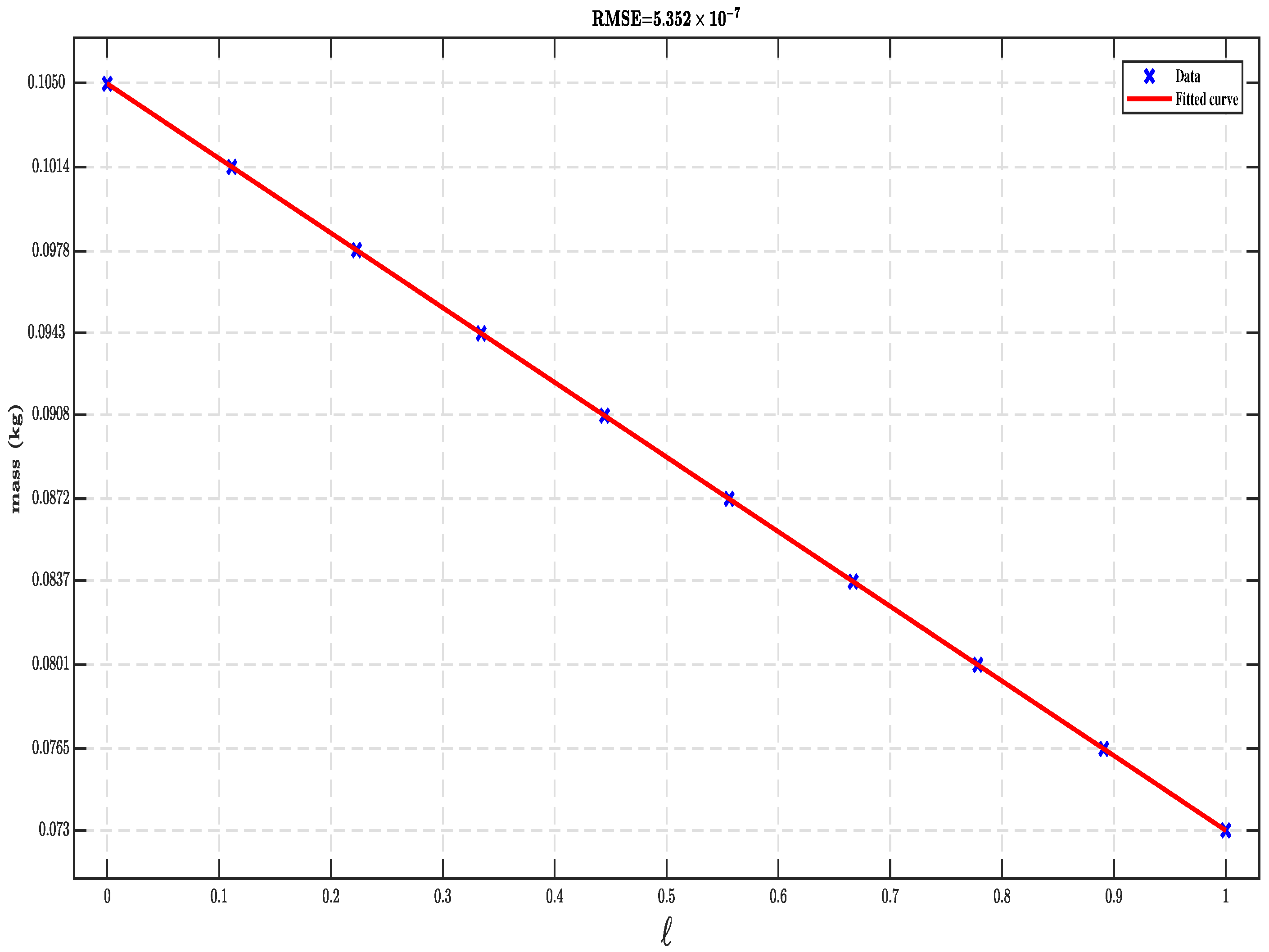
Figure 3.
Variation in mass with parameter ℓ.
Figure 3.
Variation in mass with parameter ℓ.
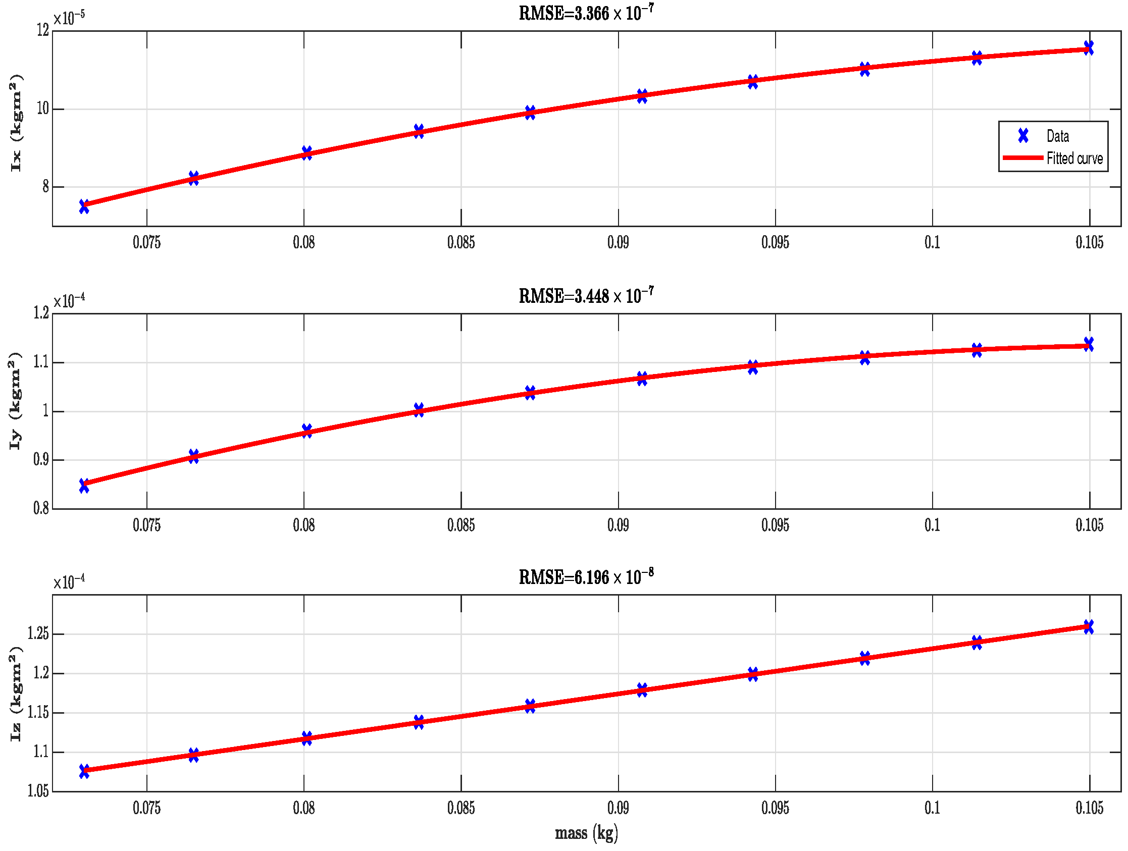
Figure 4.
Variation in MOI with mass.
Figure 4.
Variation in MOI with mass.
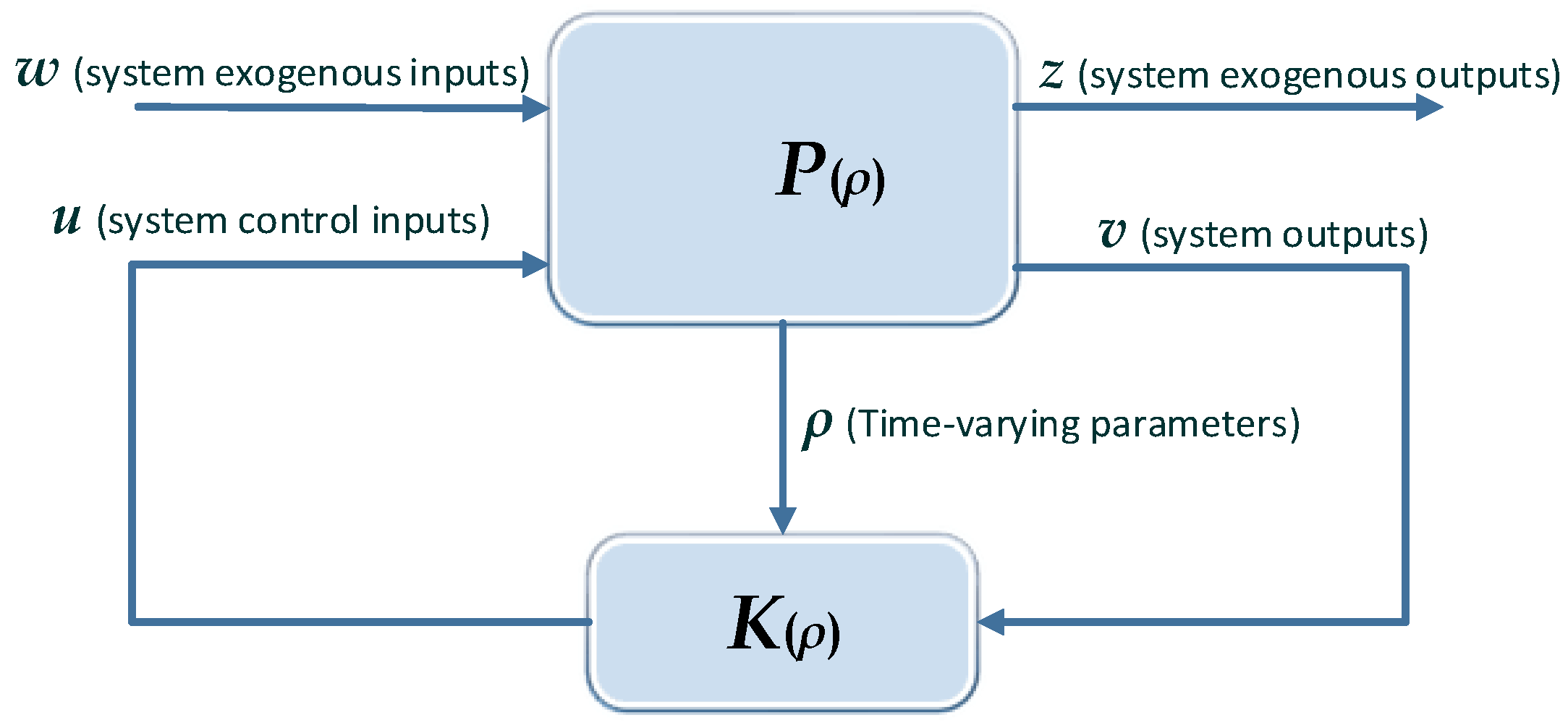
Figure 5.
The structure of closed-loop LPV system.
Figure 5.
The structure of closed-loop LPV system.
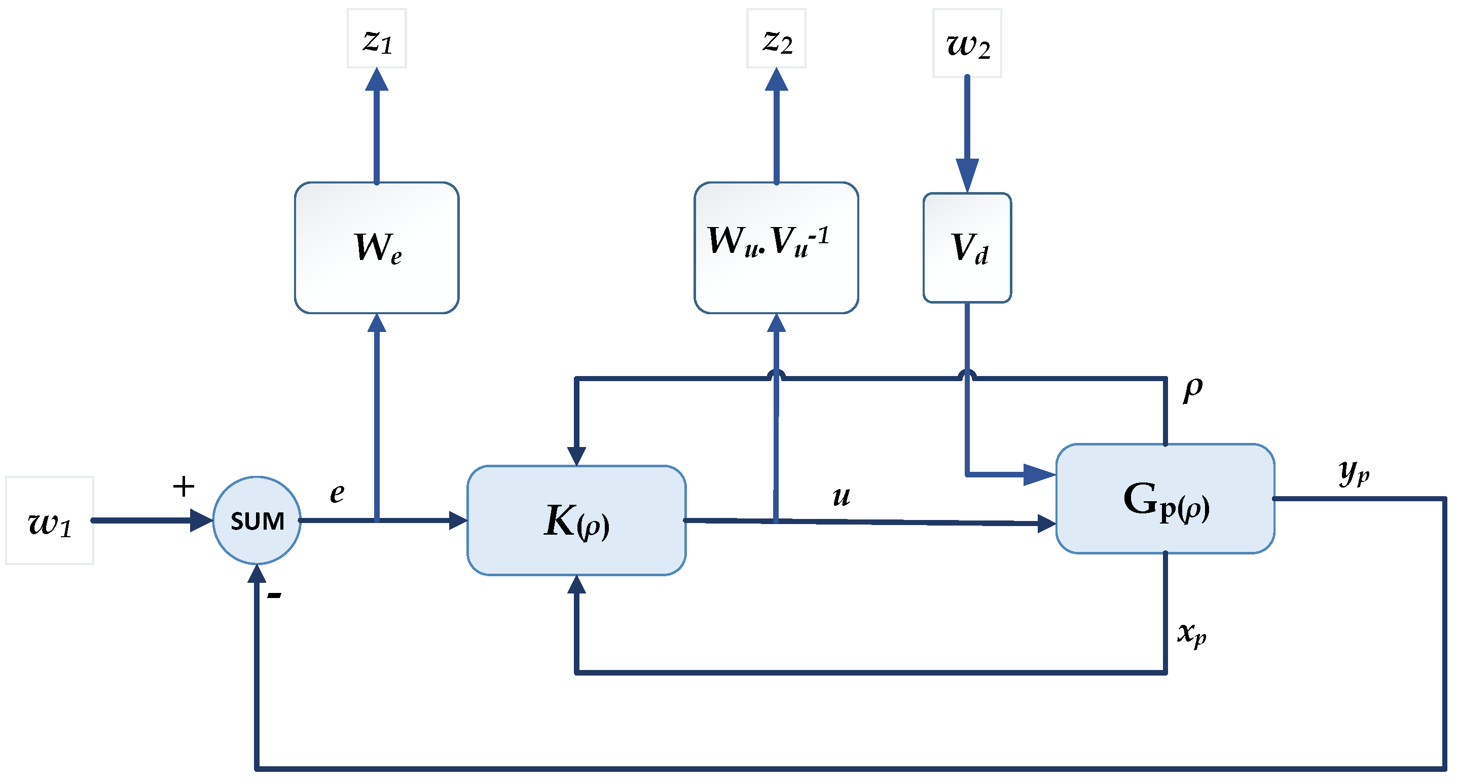
Figure 6.
The mixed sensitivity control problem.
Figure 6.
The mixed sensitivity control problem.
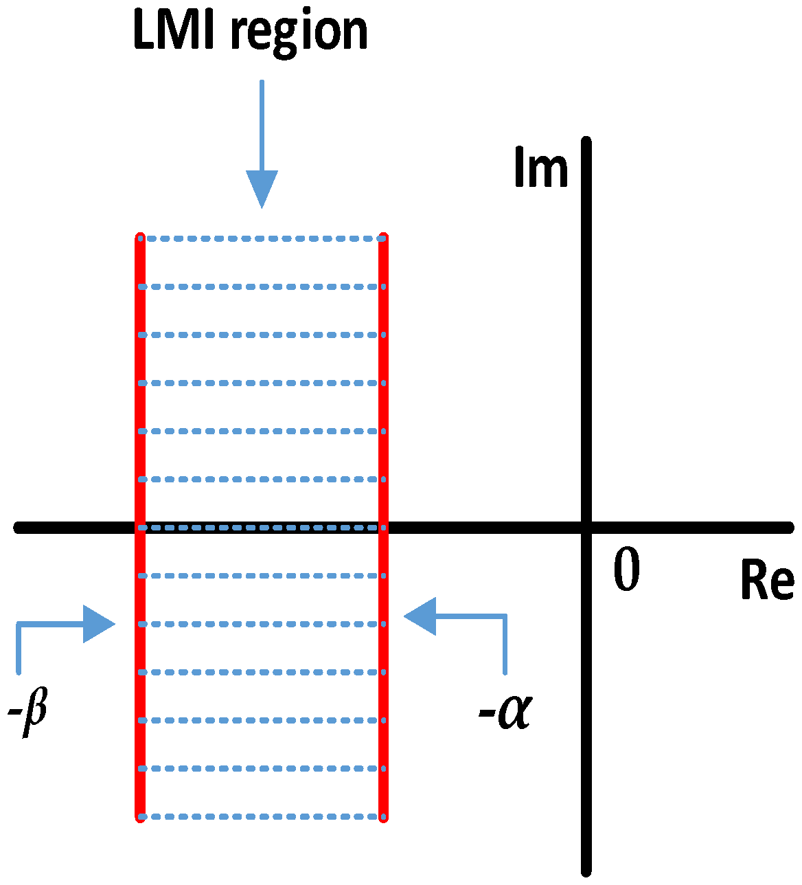
Figure 7.
Strip region .
Figure 7.
Strip region .
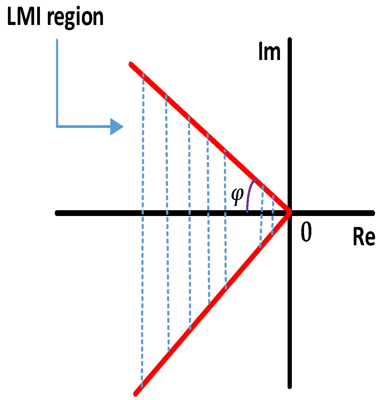
Figure 8.
Conic sector .
Figure 8.
Conic sector .
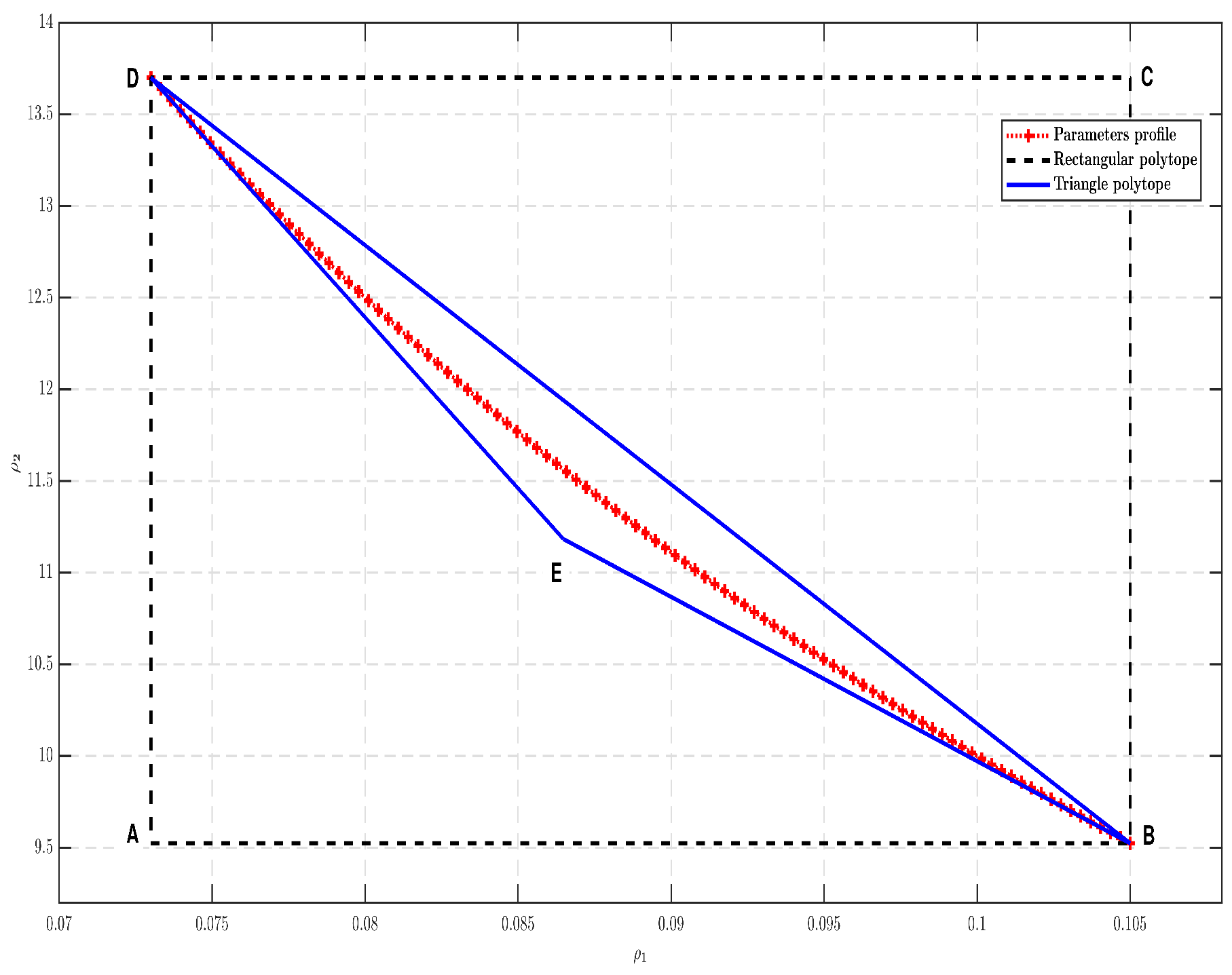
Figure 9.
The structure of the Polytopes.
Figure 9.
The structure of the Polytopes.
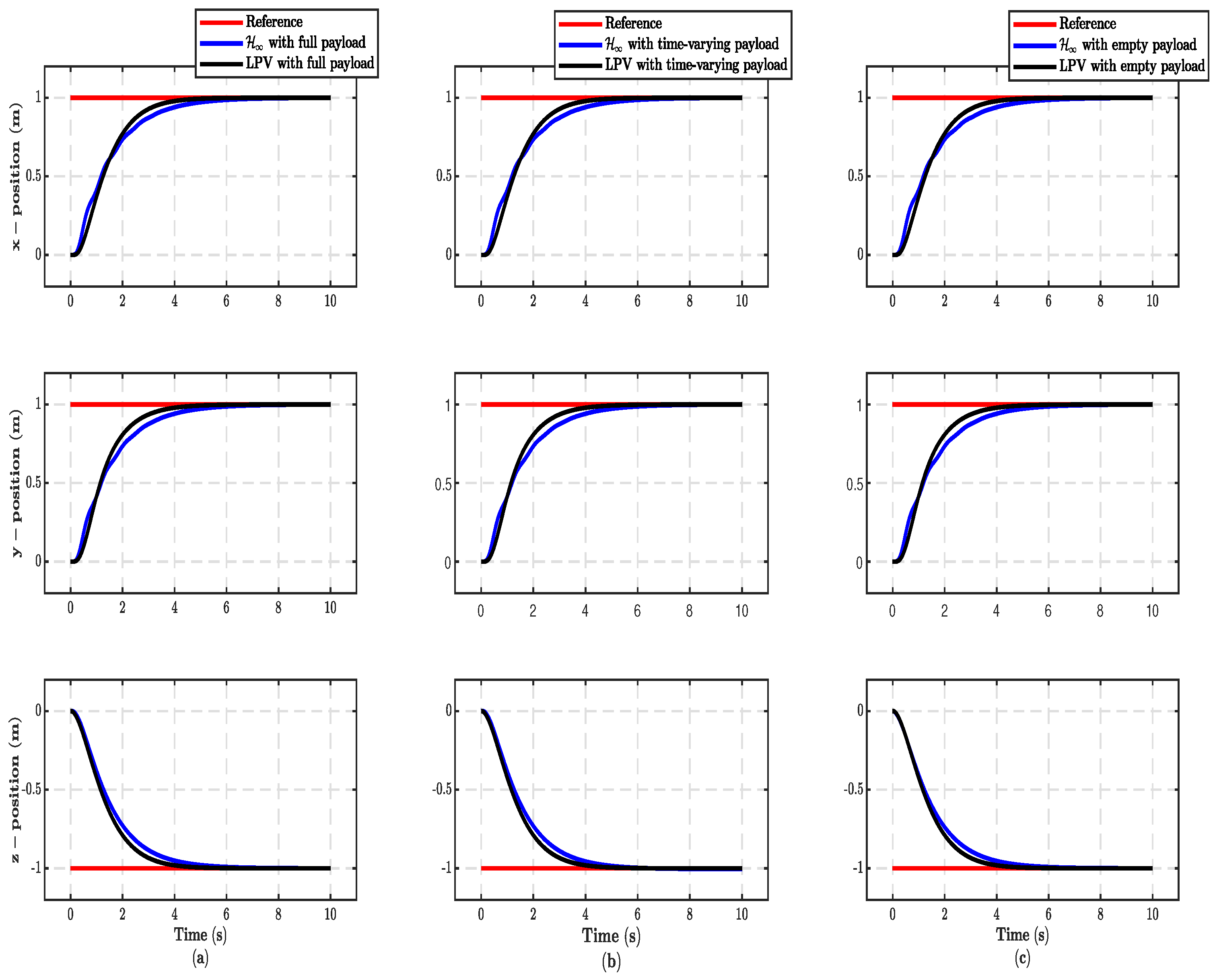
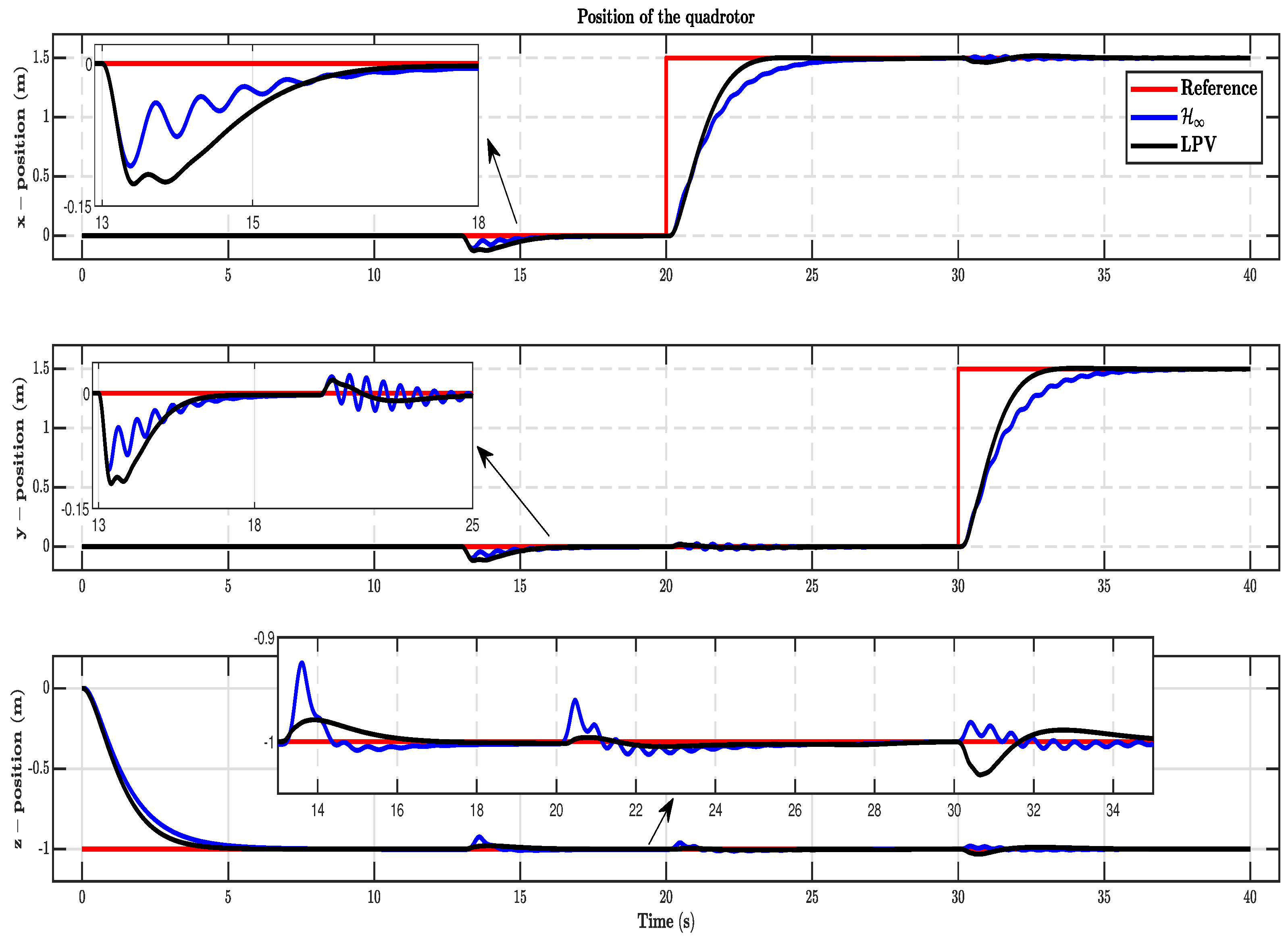
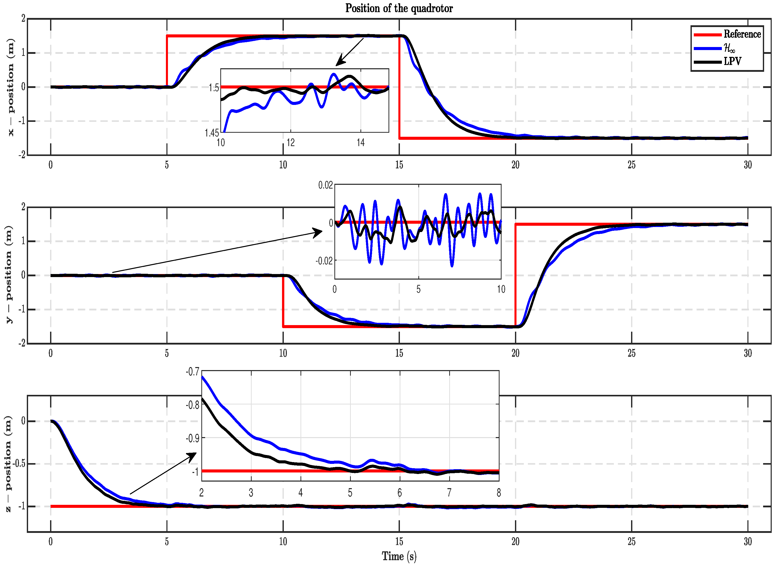
Figure 10.
(a) The positions [] with full payload; (b) The positions [] with time-varying payload; (c) The positions [] with empty payload.
Figure 10.
(a) The positions [] with full payload; (b) The positions [] with time-varying payload; (c) The positions [] with empty payload.
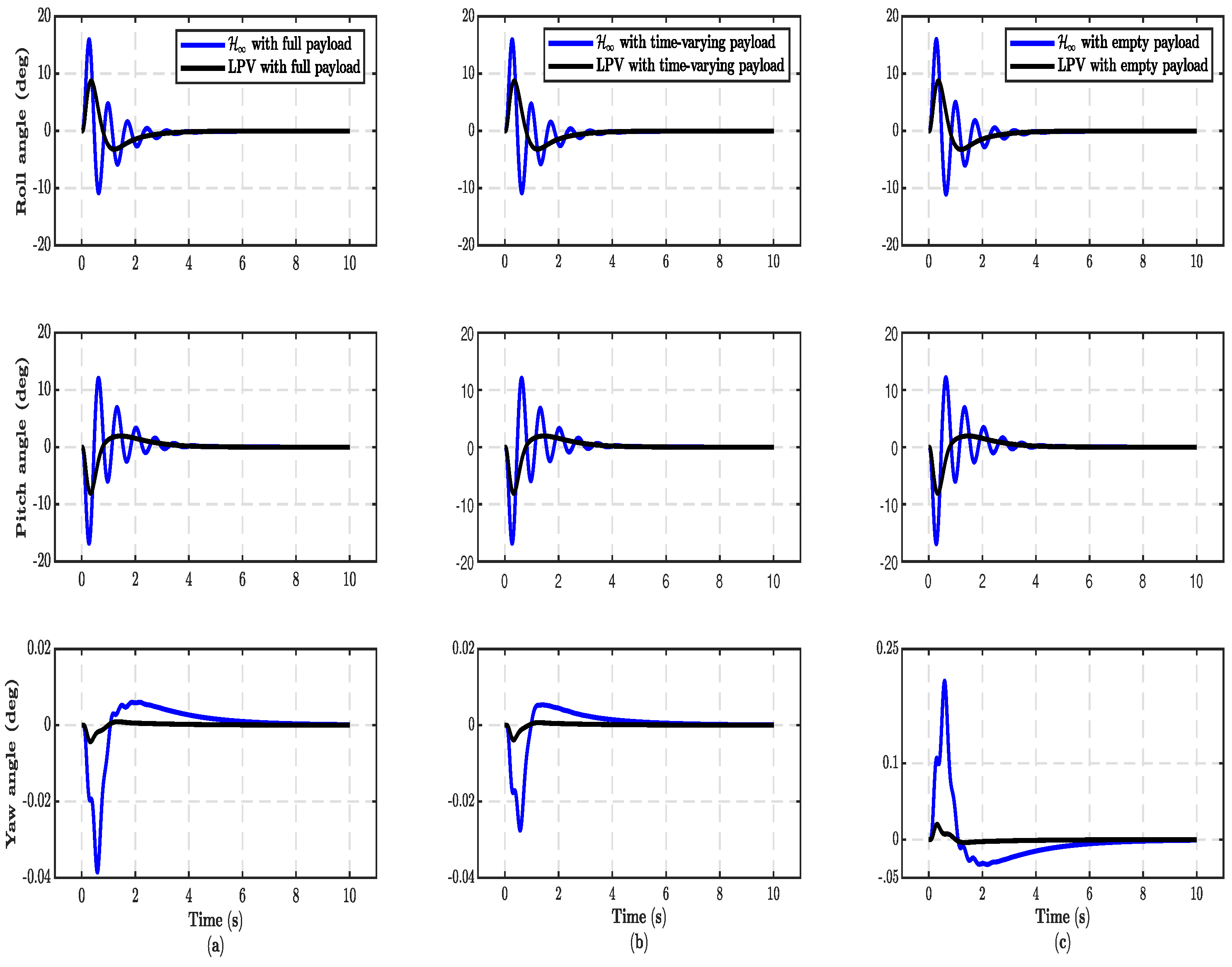
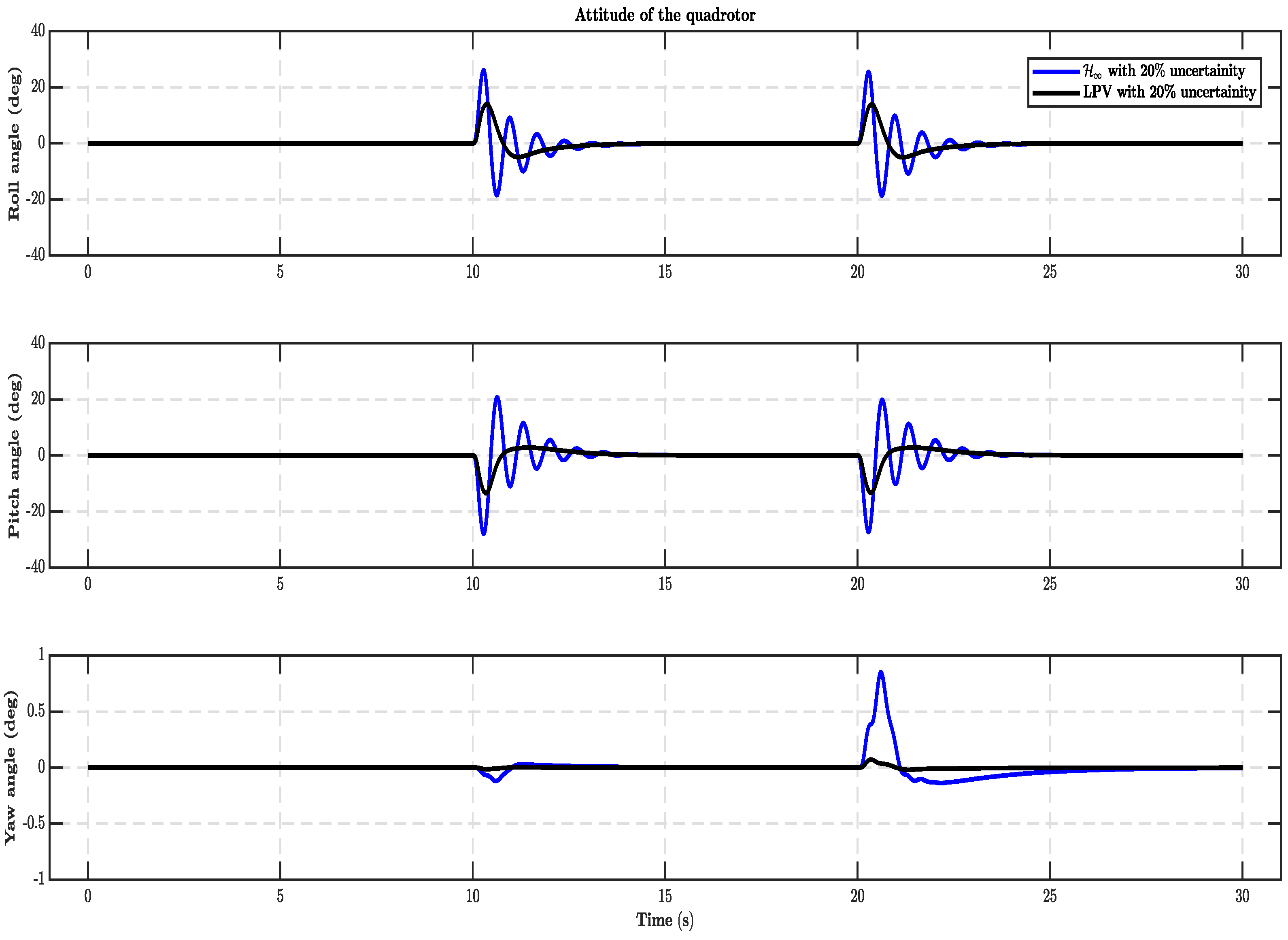
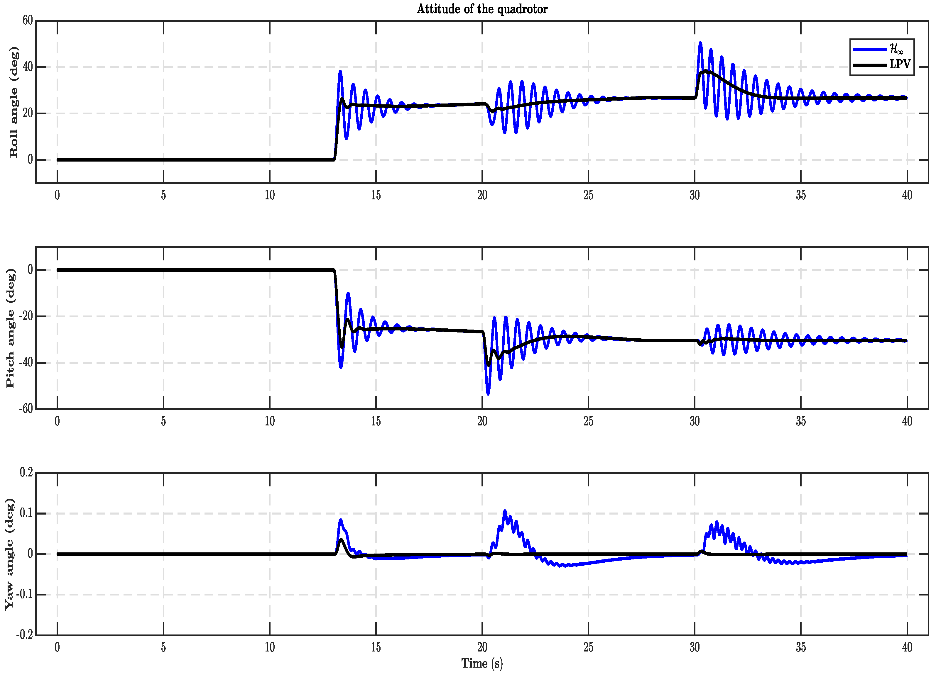
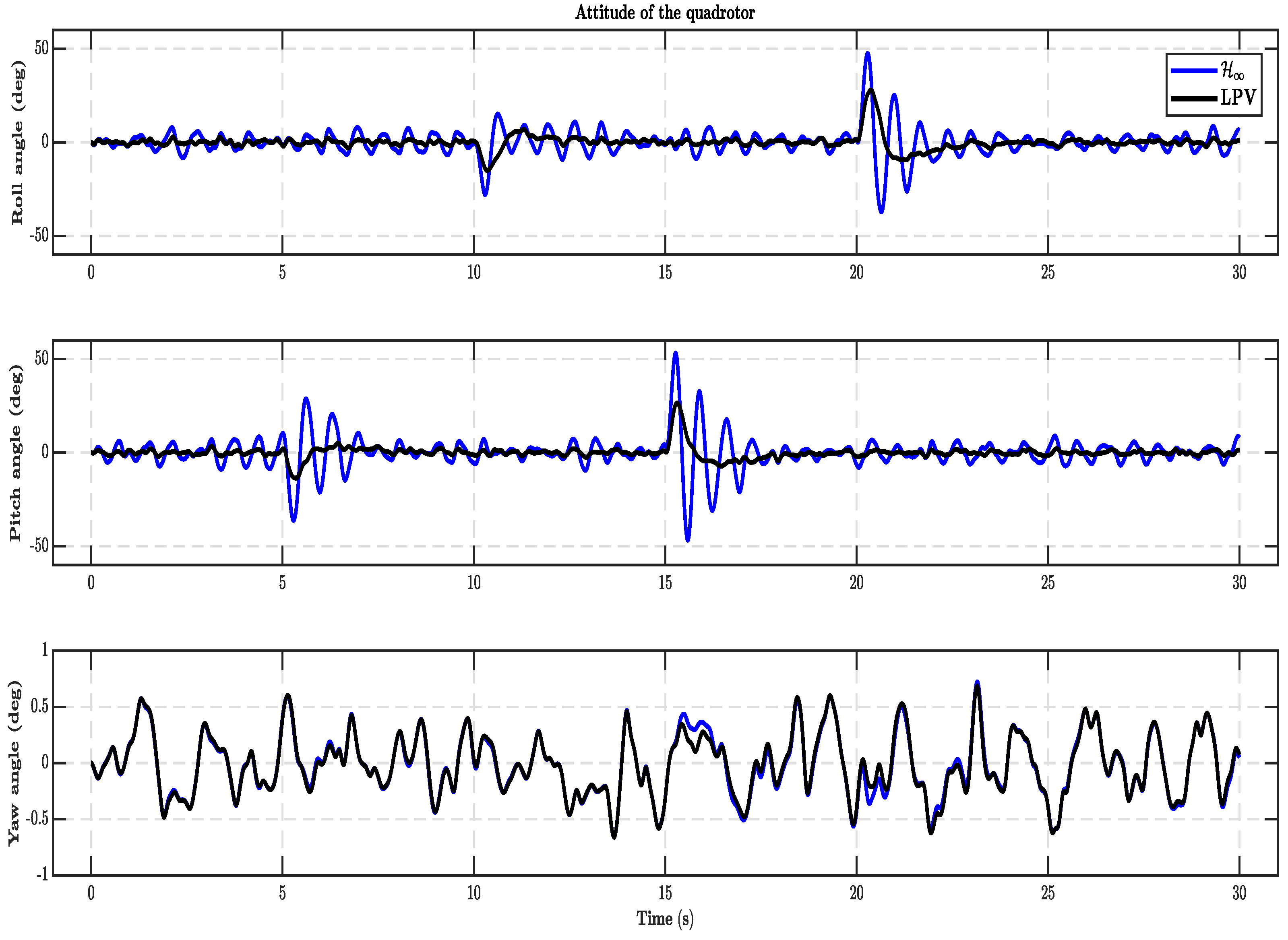
Figure 11.
(a) The attitude angles [] with full payload; (b) The attitude angles [] with time-varying payload; (c) The attitude angles [] with empty payload.
Figure 11.
(a) The attitude angles [] with full payload; (b) The attitude angles [] with time-varying payload; (c) The attitude angles [] with empty payload.
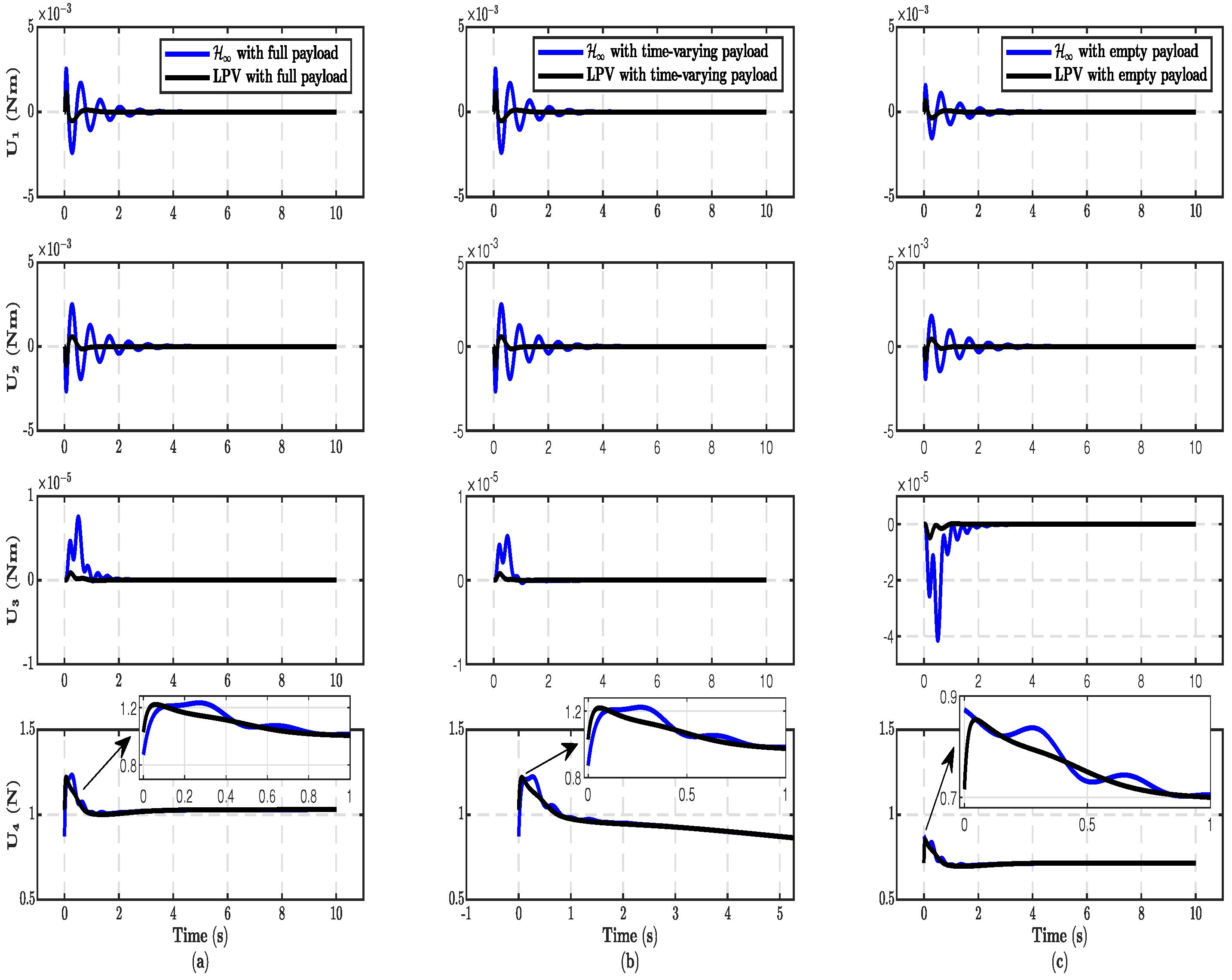
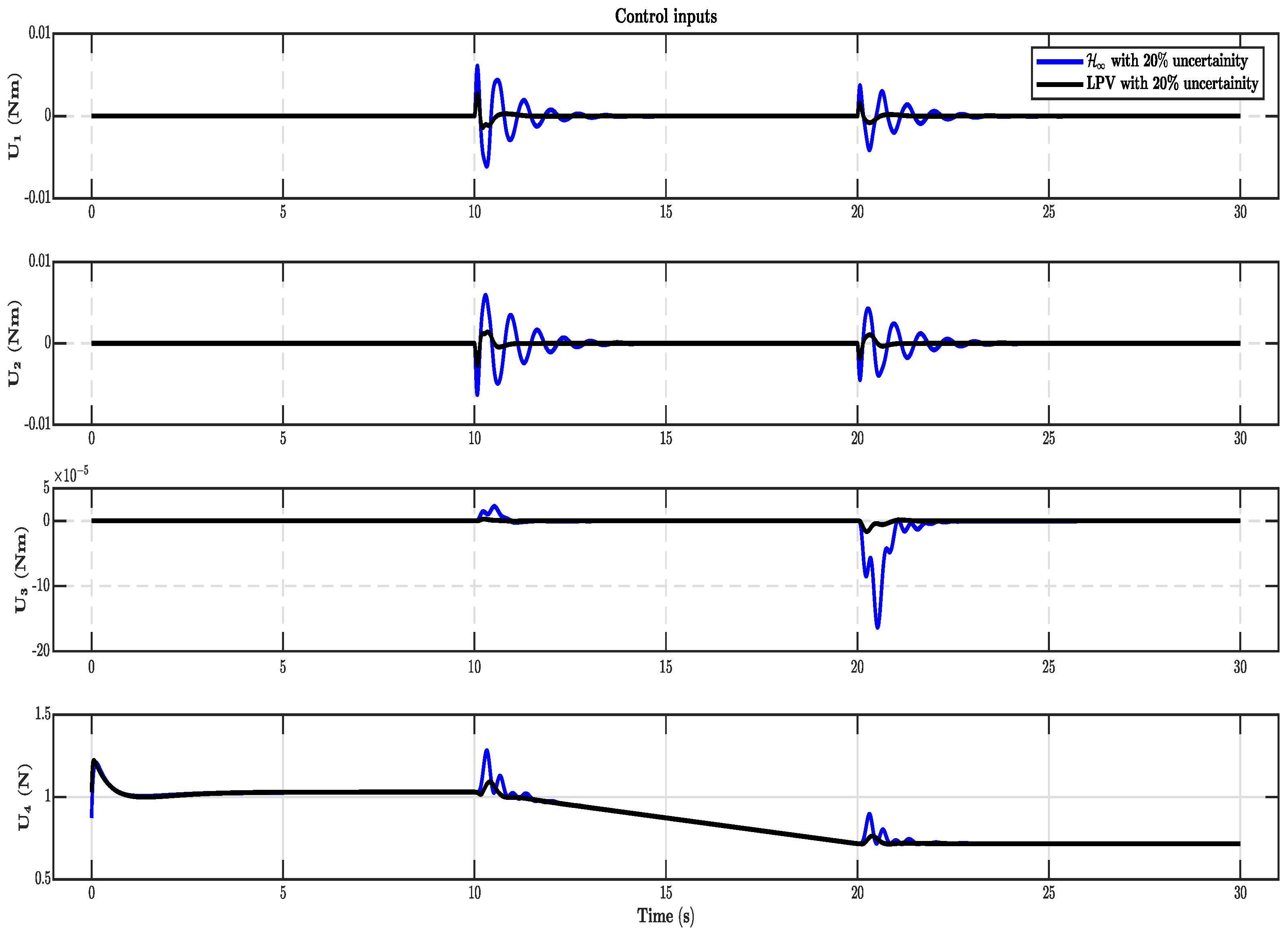
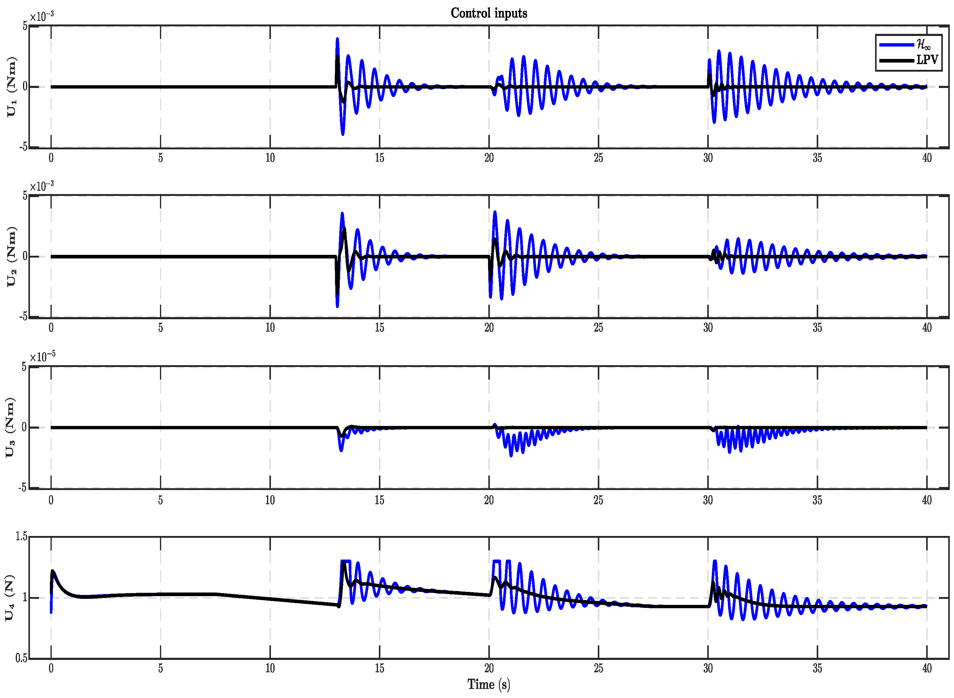
Figure 12.
(a) The control inputs [] with full payload; (b) The control inputs [] with time-varying payload; (c) The control inputs [] with empty payload.
Figure 12.
(a) The control inputs [] with full payload; (b) The control inputs [] with time-varying payload; (c) The control inputs [] with empty payload.
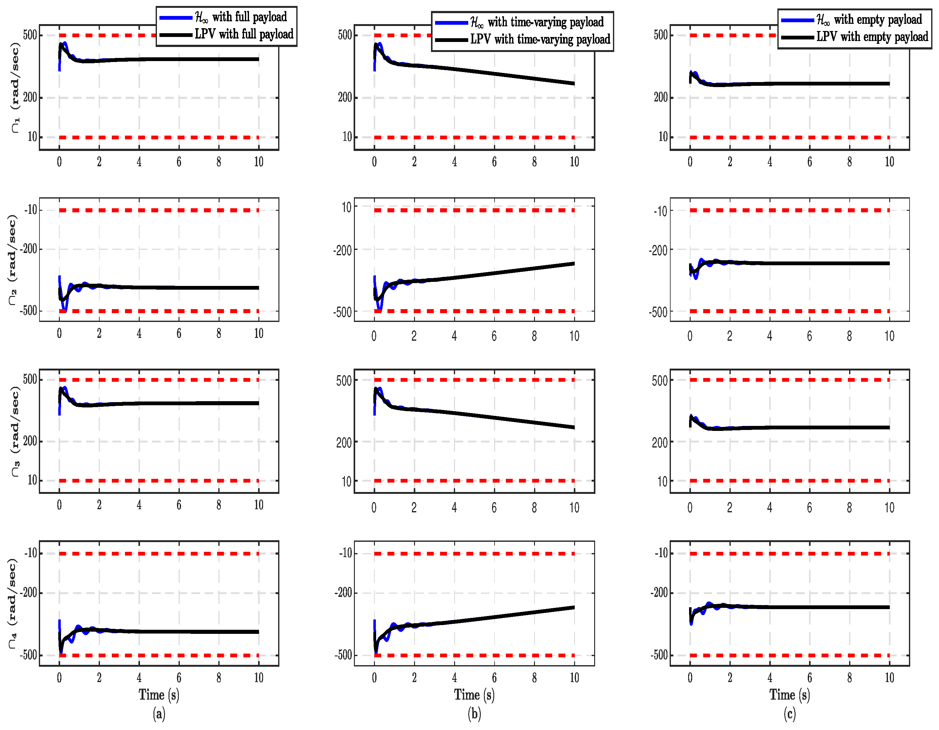
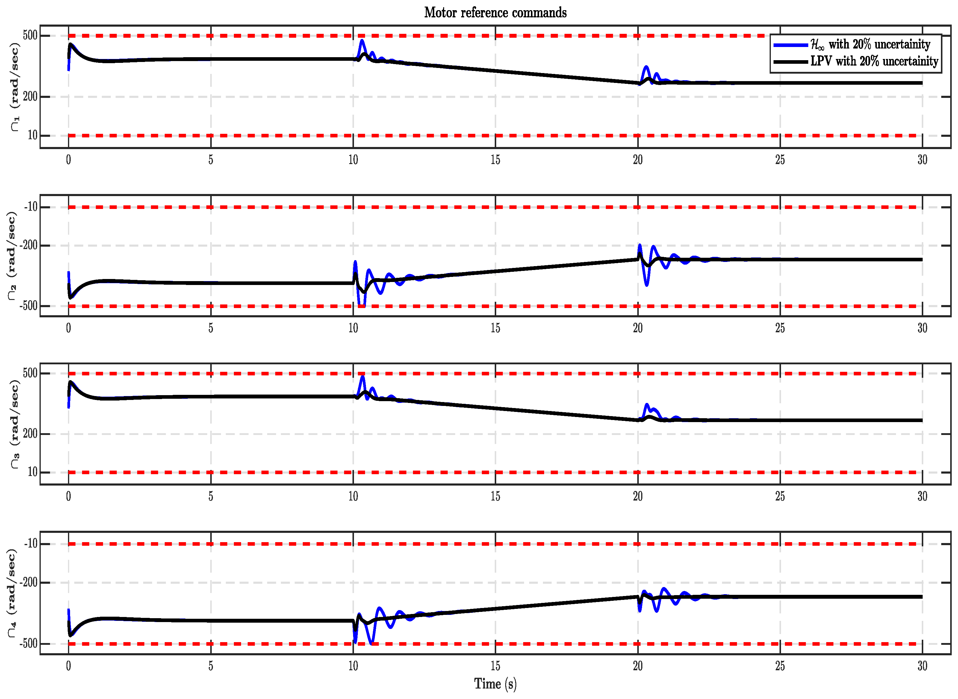
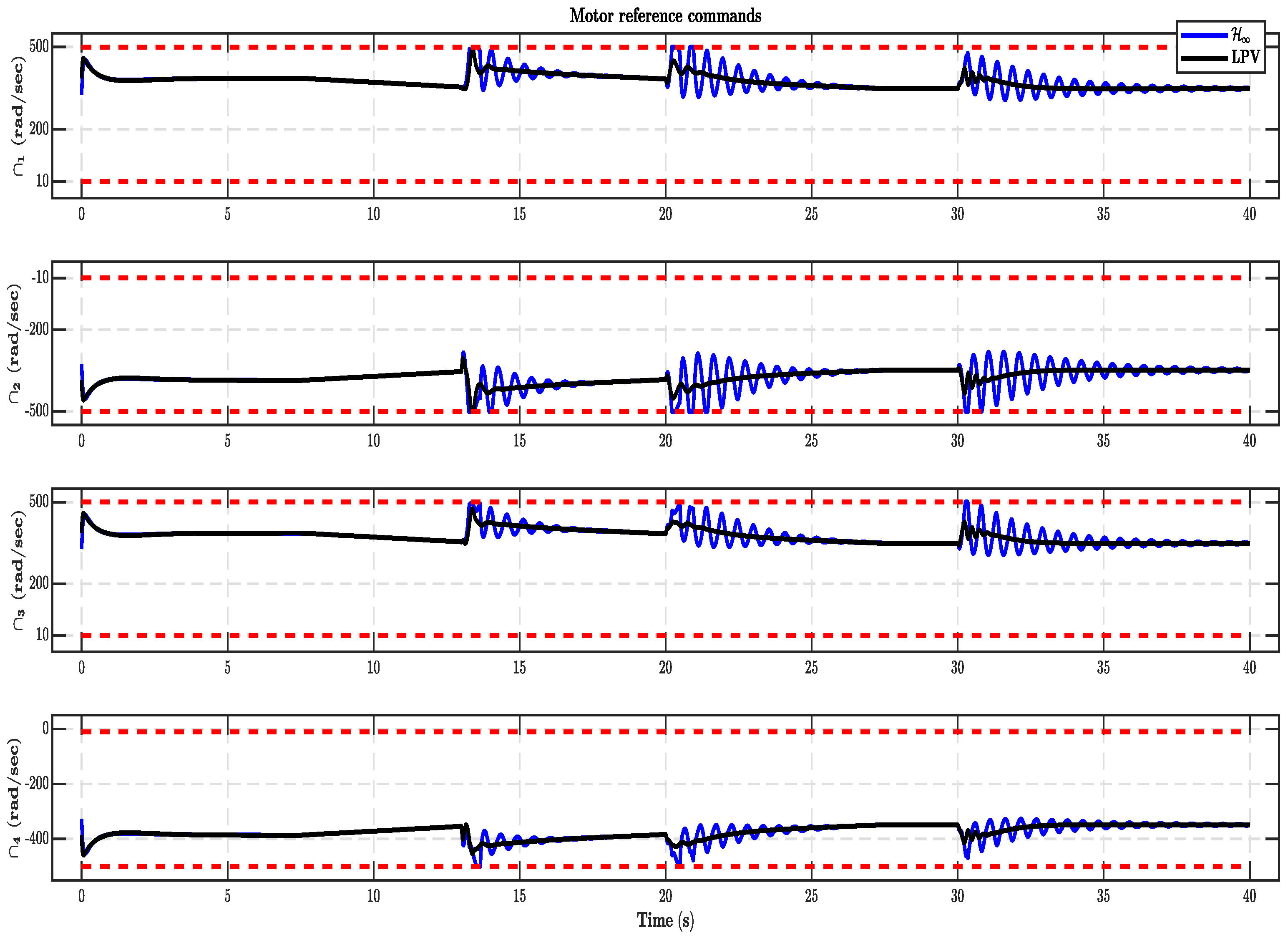
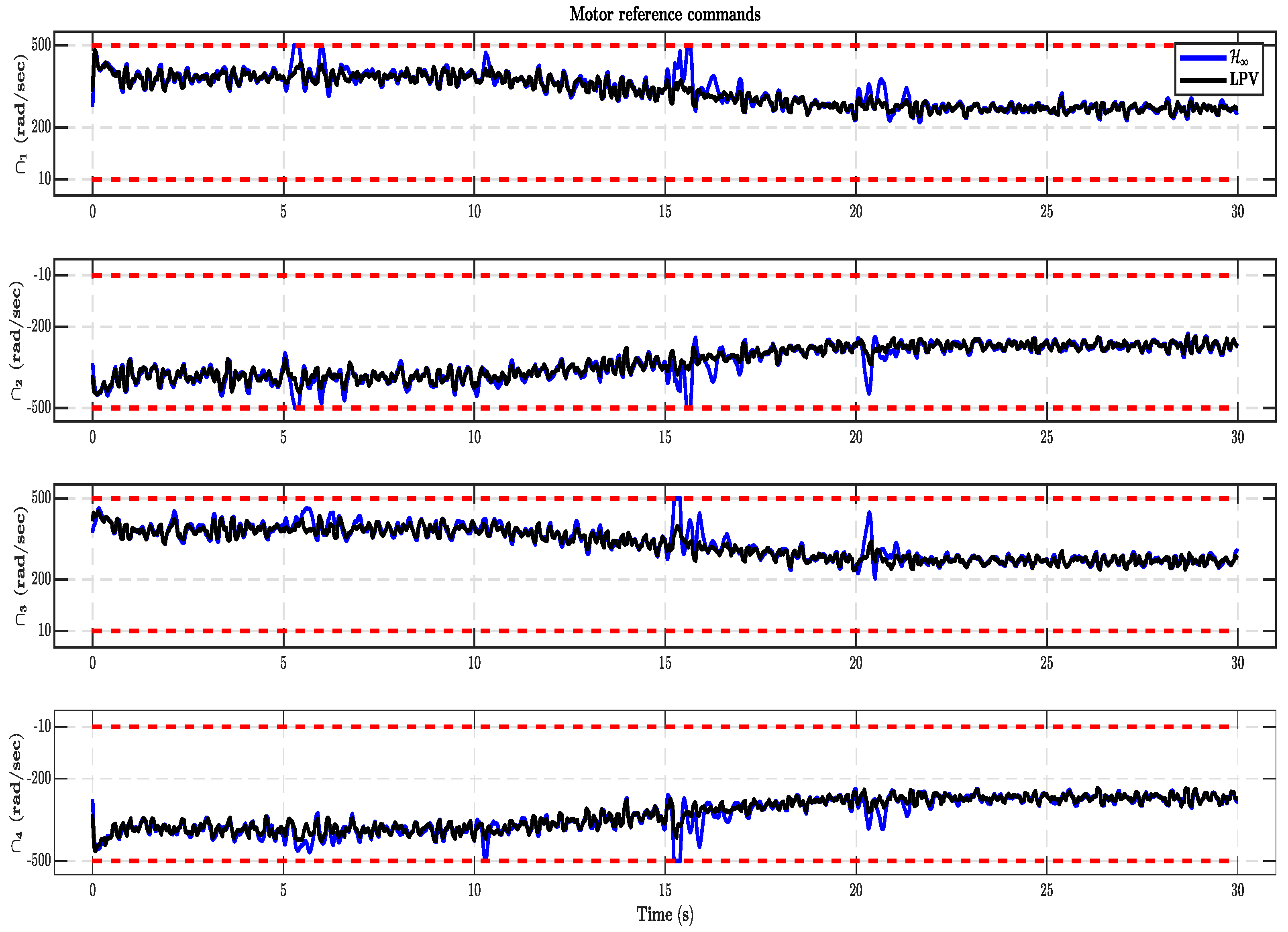
Figure 13.
(a) The motor commands [] with full payload; (b) The motor commands [] with time-varying payload; (c) The motor commands [] with empty payload.
Figure 13.
(a) The motor commands [] with full payload; (b) The motor commands [] with time-varying payload; (c) The motor commands [] with empty payload.
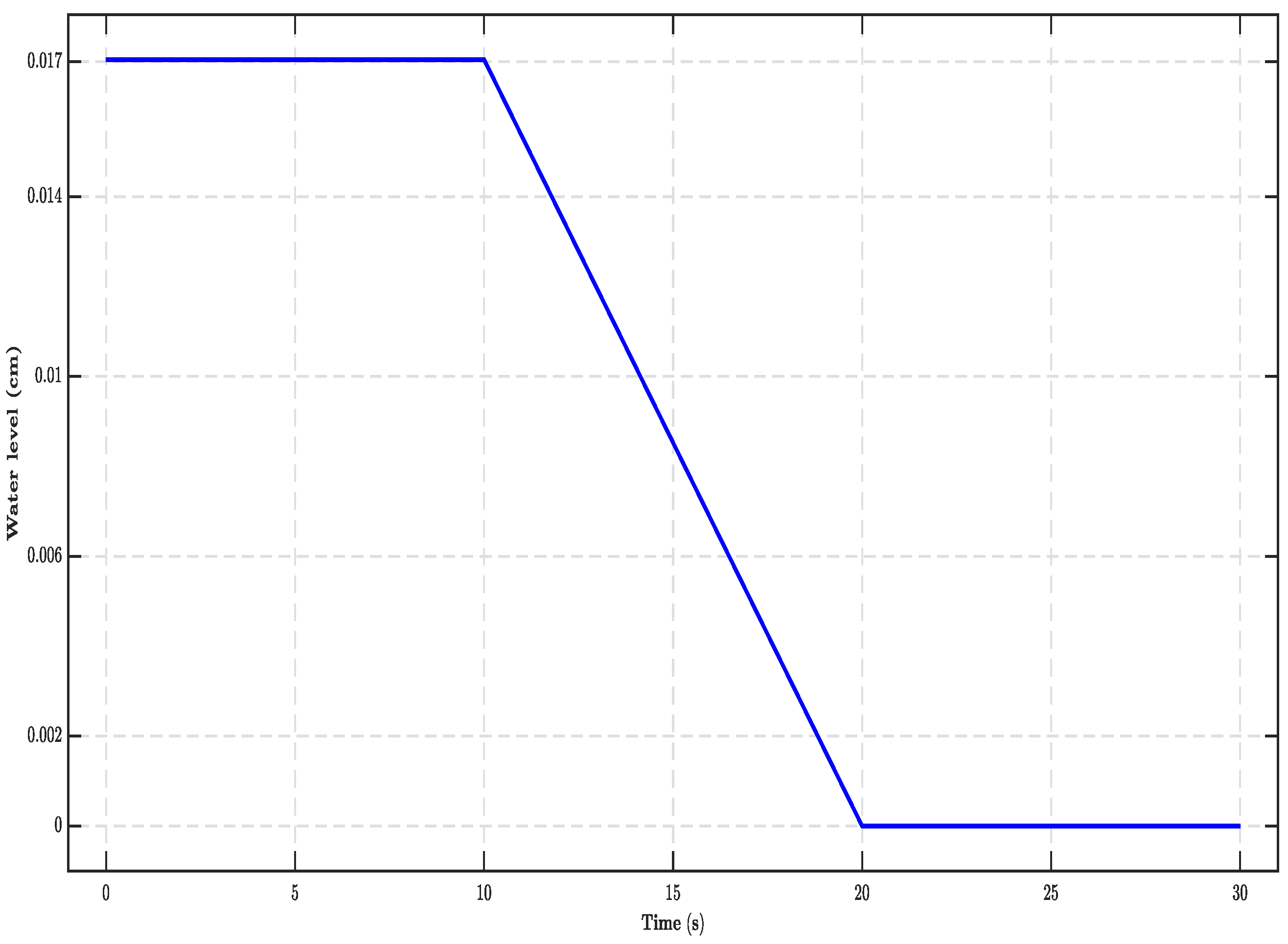
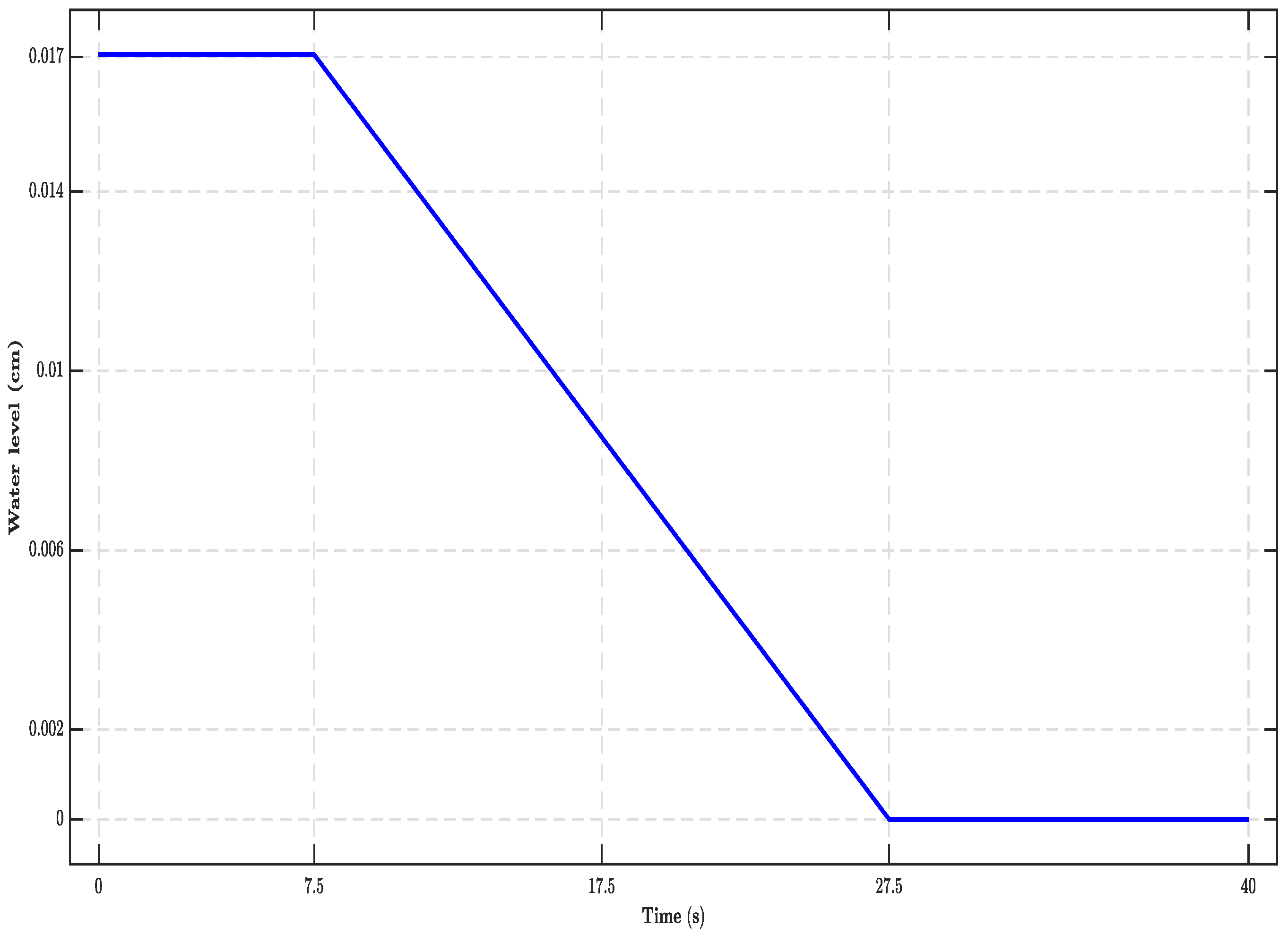
Figure 14.
Variation in the water level with time.
Figure 14.
Variation in the water level with time.
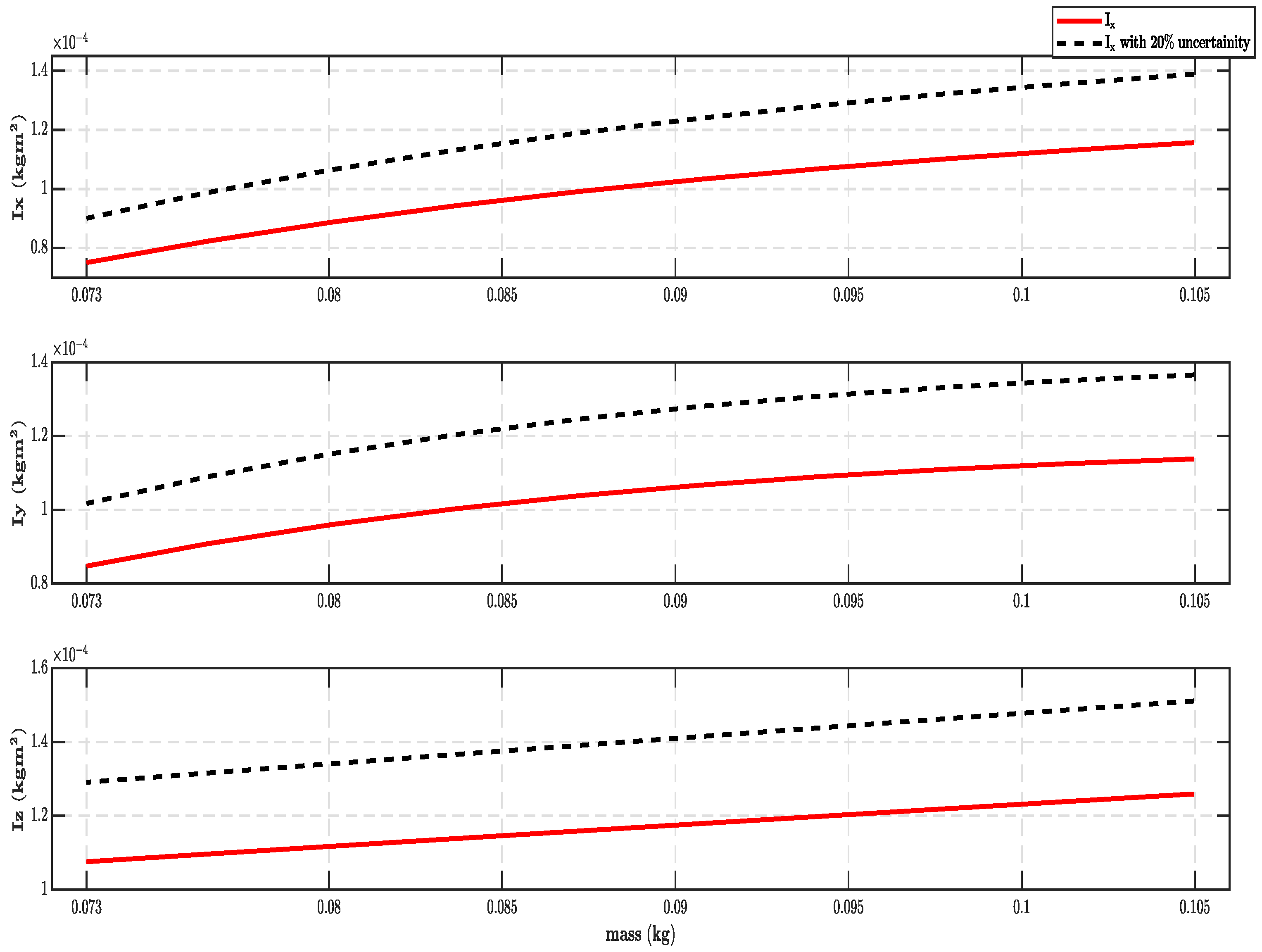
Figure 15.
Variation in the inertia parameters with mass.
Figure 15.
Variation in the inertia parameters with mass.
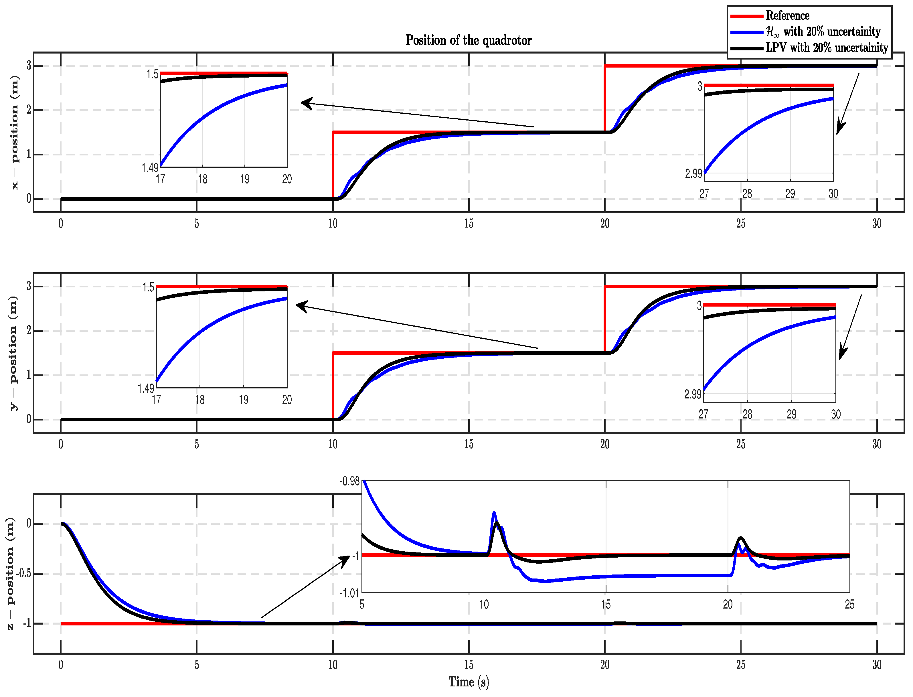
Figure 16.
The positions [] with variation in the inertia.
Figure 16.
The positions [] with variation in the inertia.
Figure 17.
The attitude angles [] with variation in the inertia.
Figure 17.
The attitude angles [] with variation in the inertia.
Figure 18.
The control inputs [] with variation in the inertia.
Figure 18.
The control inputs [] with variation in the inertia.
Figure 19.
The motor commands [] with variation in the inertia.
Figure 19.
The motor commands [] with variation in the inertia.
Figure 20.
Variation in the water level with time.
Figure 20.
Variation in the water level with time.
Figure 21.
The positions [] with payload variation and wind disturbance.
Figure 21.
The positions [] with payload variation and wind disturbance.
Figure 22.
The attitude angles [] with payload variation and wind disturbance.
Figure 22.
The attitude angles [] with payload variation and wind disturbance.
Figure 23.
The control inputs [] with payload variation and wind disturbance.
Figure 23.
The control inputs [] with payload variation and wind disturbance.
Figure 24.
The motor commands [] with payload variation and wind disturbance.
Figure 24.
The motor commands [] with payload variation and wind disturbance.
Figure 25.
The positions [] with payload variation and noise.
Figure 25.
The positions [] with payload variation and noise.
Figure 26.
The attitude angles [] with payload variation and noise.
Figure 26.
The attitude angles [] with payload variation and noise.
Figure 27.
The control inputs [] with payload variation and noise.
Figure 27.
The control inputs [] with payload variation and noise.
Figure 28.
The motor commands [] with payload variation and noise.
Figure 28.
The motor commands [] with payload variation and noise.
Table 1.
Quadrotor parameters with full payload.
Table 1.
Quadrotor parameters with full payload.
| Quantity | Symbol | Value | Unit |
|---|
| Mass of quadrotor | | | kg |
| Inertia about the x-axis | | | kg m2 |
| Inertia about the y-axis | | | kg m2 |
| Inertia about the z-axis | | | kg m2 |
| Length of an arm | l | | m |
| Rotor inertia | | | kg m2 |
| Drag factor | | | kg/m |
| Drag factor | | | kg/m |
| Thrust coefficient | | | N/(rad2/s2) |
| Thrust coefficient | | | Nm/(rad2/s2) |
| Acceleration of gravity | | 9.81 | m/s2 |
Table 2.
Mass and inertia values at different water levels.
Table 2.
Mass and inertia values at different water levels.
| S.No | Water Level (m) | Mass (kg) | | | |
|---|
| 1 | | | | | |
| 2 | | | | | |
| 3 | | | | | |
| 4 | | | | | |
| 5 | | | | | |
| 6 | | | | | |
| 7 | | | | | |
| 8 | | | | | |
| 9 | | | | | |
| 10 | 0 | | | | |
Table 3.
Parameter values.
Table 3.
Parameter values.
| Parameter | Value | Unit |
|---|
| | kg |
| | kg |
| | m2/kg |
| | m2 |
| | kg m2 |
| | m2/kg |
| | m2 |
| | kg m2 |
| | m2 |
| | kg m2 |
Table 4.
and values of fully actuated subsytem.
Table 4.
and values of fully actuated subsytem.
| Name | z-Position | Yaw Angle |
|---|
| | |
| | |
Table 5.
and values of under-actuated subsytem.
Table 5.
and values of under-actuated subsytem.
| Name | Roll Angle | Pitch Angle | x-Position | y-Position |
|---|
| | | | |
| | | | |
Table 6.
The closed-loop performance parameters with full payload.
Table 6.
The closed-loop performance parameters with full payload.
| | Performance Parameters | LPV | | % Improvement |
|---|
| x-position | | s | s | 6.96275 |
| s | s | |
| OS | | | 0 |
| MSE | m | m | |
| y-position | | s | s | |
| s | s | |
| OS | | | 0 |
| MSE | m | m | |
| z-position | | s | s | |
| s | s | |
| OS | | | 0 |
| MSE | m | m | |
Table 7.
The closed-loop performance parameters with time-varying payload.
Table 7.
The closed-loop performance parameters with time-varying payload.
| | Performance Parameters | LPV | | % Improvement |
|---|
| x-position | | s | s | |
| s | s | |
| OS | | | 0 |
| MSE | m | m | |
| y-position | | s | s | |
| s | s | |
| OS | | | 0 |
| MSE | m | m | |
| z-position | | s | s | |
| s | s | |
| OS | | | 0 |
| MSE | m | m | |
Table 8.
The closed-loop performance parameters with empty payload.
Table 8.
The closed-loop performance parameters with empty payload.
| | Performance Parameters | LPV | | % Improvement |
|---|
| x-position | | s | s | |
| s | s | |
| OS | | | 0 |
| MSE | m | m | |
| y-position | | s | s | |
| s | s | |
| OS | | | 0 |
| MSE | m | m | |
| z-position | | s | s | |
| s | s | |
| OS | | | 0 |
| MSE | m | m | |


