An Innovative System of Deep In Situ Environment Reconstruction and Core Transfer

Featured Application

Only when deep in situ rock samples are tested in the same environments as their occurrences can their true physical and mechanical properties be obtained. Therefore, a fidelity test system that can simulate the deep in situ geological conditions has become an urgent need to promote the deep in situ rock mechanics. This work is the key component of the fidelity test system, being used to accurately reconstruct a deep in situ high-temperature and high-pressure environment in the system.

Abstract

The reconstruction of deep in situ environment up to 95 °C and 70 MPa using water is critical for the fidelity testing of deep Earth rocks. The temperature and pressure of the water have strong coupling in such an environment, which makes the control of temperature and pressure very difficult. The paper firstly presents the design of the system of deep in situ environment reconstruction and core transfer (SERCT); secondly, for the problem of high temperature and pressure control, a pressure-temperature (P-T) interpolation control algorithm based on the iso–density P-T curves of water is proposed. A P-T coupling control path is decomposed into two independent interpolation paths: an iso–thermal pressure control and an iso–mass temperature control, which realizes the decoupling control of temperature and pressure. Then, a fuzzy-PID dual mode method is adopted for the pressure control after decoupling, which reduces the overshoot and the dynamic response time of the system. For temperature control, a segmented and grouped electric heating mode is designed to improve the uniformity of the temperature field. A fuzzy PID temperature control algorithm based on grey prediction is proposed to achieve high precision temperature control with small overshoot. Finally, the effectiveness of the proposed methods is verified by experiments.

1. Introduction

As the shallow resources are gradually exhausted, human beings began to collect resources from the deep Earth [1]. Rocks at different depths may have different physical and mechanical properties. However, currently the basic physical and mechanical properties of rocks, such as porosity, Poisson’s ratio, elastic modulus, etc., are obtained by empirical rock mechanics theory and experimental methods based on standard cores, in which the effects of deep in situ environment, such as temperature and pressure, are not considered, and the obtained parameters, mathematical models and theories are independent of the occurrence depth of rocks [2,3].

Therefore, it is necessary to analyze the physical and mechanical behaviors of rocks in the deep in situ environment, and develop a rock mechanics theory that considers the influence of the deep in situ environment [4]. To achieve this goal, a platform that can reconstruct and simulate the deep in situ environment of high temperature and high pressure—and complete the transfer, preparation and testing of the core in this environment—is essential. One key difficulty in the development of this platform is the control of temperature and pressure, because under high temperature and pressure, the temperature and the pressure affect each other, and the movement of core may cause great fluctuations in pressure and temperature.

In this study, the SERCT is designed to reconstruct a deep in situ environment of 2500 m underground. At this depth, the temperature is approximately 95 °C and the pressure is highly likely to be less than 70 MPa. A P-T decoupling control method is then proposed to achieve the in situ environment reconstruction with high temperature (up to 95 °C) and high pressure (up to 70 MPa). For the independent controls of pressure and temperature after decoupling, a fuzzy-PID dual mode pressure control and a fuzzy PID temperature control based on grey prediction are presented.

2. Related Works

Deep in situ environment reconstruction is mainly used in the field of deep Earth and deep sea science research to build the deep in situ environment with specific temperature and pressure [5]. Researchers in the United States, Japan, Russia, South Korea, etc., began their study early in this field and have achieved significant results [6].

As early as 1951, a U.S. naval shipyard built a deep sea pressure simulation device, achieving a cyclic pressurization of 0.1–4 MPa with a maximum pressure of 4.2 MPa [7]. After that, a device with a maximum pressure of 82.75 MPa was developed [8]. A periodic pressure test device with a maximum pressure of 156 MPa was developed in Japan [9]. Furthermore, a medium-sized chamber was subsequently developed to simulate the dynamic pressure environment up to 154.9 MPa, and its maximum working pressure in the circulation mode could reach 113.7 MPa [10]. Researchers in Russia developed a series of deep sea environment simulation platforms, which could realize the test pressure up to 150 MPa [11]. The above equipment only focused on the pressure loading, and the influence of temperature was not considered.

In the fields of P-T control and core test under the in situ fidelity environment, researchers in the U.K., E.U., U.S. and China have achieved impressive results [12]. The MSCL system developed by Geotek in 2003 could be used for parametric analysis of cores or seafloor sediments. Although this system was not strictly a fidelity system, it helped to accumulate rich experience in core transfer under in situ fidelity environment [13,14]. In 2009, Geotek developed the PCATS system on the basis of MSCL, which could achieve a maximum pressure of 35 MPa and a temperature control of 4–20 °C. The HYACINTH system developed in Europe could cut, transfer and test samples in an in situ pressure environment with a maximum pressure of 25 MPa [15]. The pressure-holding transfer device for natural gas hydrate developed by Zhejiang University in China could achieve fidelity testing at a temperature of 2–4 °C and a pressure of up to 30 MPa [16].

In temperature and pressure control, many control methods have been produced. The earlier temperature control methods such as fuzzy logic controller [17], intelligent control [18] and cascade controller [19] all have good performance, but their computational efficiency and stability need to be further improved. Recently, temperature control methods based on prediction began to attract attention. The prediction-based methods have a good performance in improving response speed and reducing overshoot. Shakeri et al. proposed an intelligent random model prediction method, which used path integration method and particle swarm optimization algorithm to achieve optimal control of temperature [20]. Shi et al. proposed a delay-range-dependent robust constrained model predictive control method, which had better track and anti-interference performance for temperature control [21]. Aguilar et al. proposed a dual input and dual output predictive control strategy, which improved the production efficiency of temperature control [22]. In terms of pressure control, on the basis of the early standard PID control method, a lot of improved methods, such as fuzzy PID control, BP neural network control, and PID control based on ant colony algorithm, have been developed [23,24]. These methods generally have better performance than the conventional PID method. In the decoupling control of pressure and temperature, researchers in the chemical industry adopted the pressure-compensated temperature control method for the temperature and pressure control of mixed gas [25,26]. Zheng et al. proposed a dynamic pressure control method based on LPID, which created a scheduling table by pre calculated PID parameters, performed PID compensation under different temperature and pressure conditions, and realized stable pressure control [27].

In general, the existing research on in situ environmental reconstruction and core transfer systems needs further improvement in two aspects. On the one hand, a deep in situ simulation environment with higher temperature and higher pressure at the same time is necessary to obtain a wider range of the system applications; on the other hand, dynamic pressure and temperature control during the course of building the deep in situ environment and moving the cores, especially the P-T decoupling control under high pressure and high temperature, needs to be further explored.

3. Design of the SERCT

3.1. System Functions and Composition

The SERCT simulates the pressure and temperature of the environment where the cores stay in the deep Earth; additionally, it is the platform where the cores are moved and prepared for the fidelity physics test. The system composition is shown in Figure 1.

Figure 1. The SERCT; (a) The composition of the SERCT; (b) The actual picture of the SERCT.

As shown in Figure 1a, 1 is the push rod chamber. The push rod opens the docking chamber 3 which is the device for transporting the core from the deep Earth, grabs the core, pulls it out of the docking chamber, and transfers it between chambers. Moreover, 2 is the storage chamber used for temporary storage of the core; 4 is the non-contact test chamber for acoustic and electromagnetic tests of the core; 5 is the preparation chamber for core sample preparation; 6 is the pressure test chamber for core samples. The chambers are connected through high pressure flat gate valves.

During the core preparation and test, all the chambers are full of water whose pressure and temperature are kept the same as those inside the docking chamber. When the push rod moves or the valves open or close, the fluctuation of temperature and pressure should be less than ±3% F.S.

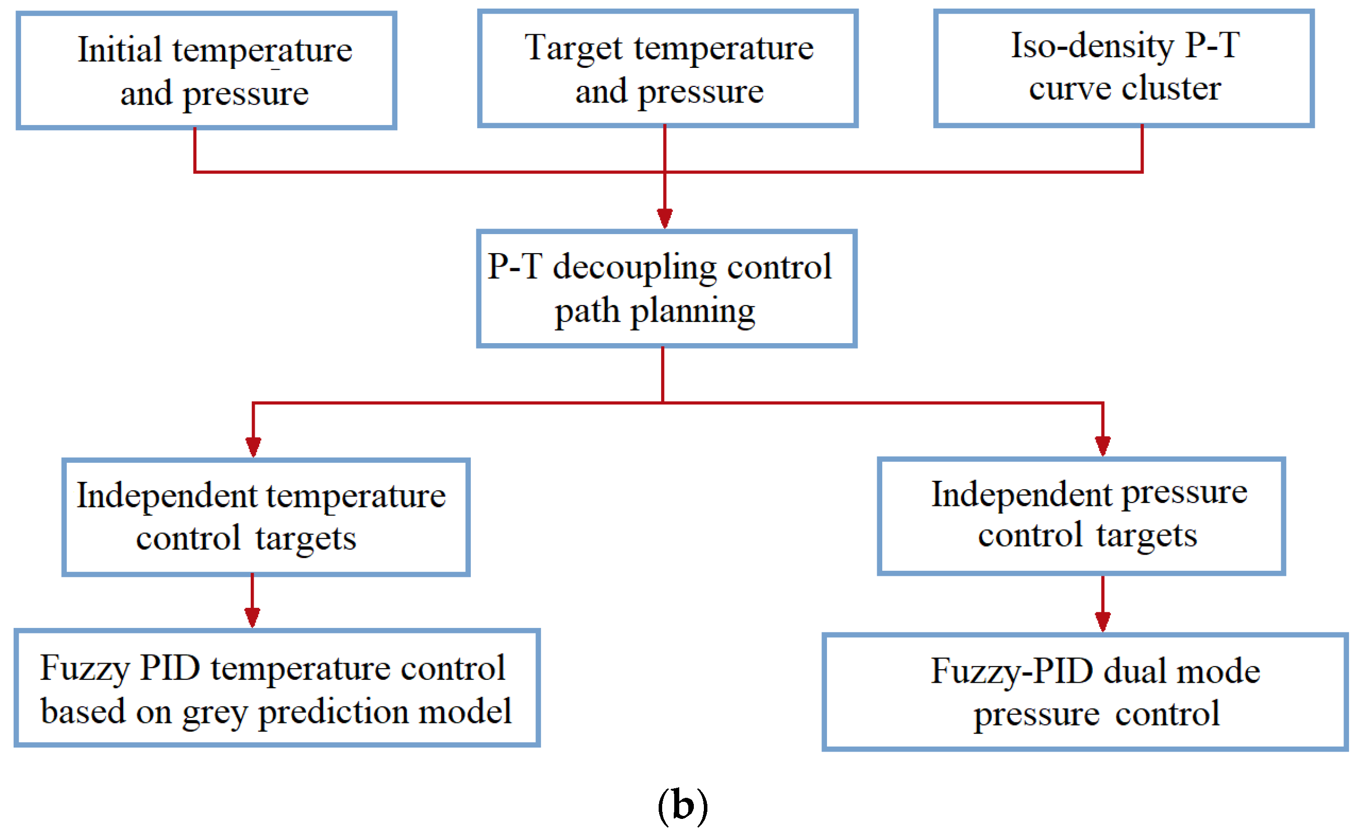
3.2. The Temperature and Pressure Decoupling Control System

The temperature and pressure control of SERCT is divided into two types: (1) Initial environment reconstruction and (2) P-T preservation. The initial environment reconstruction establishes the target deep in situ temperature and pressure in the chamber from the normal temperature and pressure, which is a heating and pressurizing process. The P-T preservation means that after the initial environment reconstruction finishes, the system needs to reduce the fluctuations of the temperature and pressure caused by the movements of the push rod and the valves.

The structure of the temperature and pressure control system is shown in Figure 2a. The loop of water includes: the working chamber, the pressure relief valve, the water tank, the preheating chamber, and the booster valve. We use a two-layer control structure for temperature and pressure control: in the inner layer, the central controller obtains the data of the temperature sensors and the pressure sensor located in the working chamber, plans the decoupling control targets of temperature and pressure based on the sensor data and transmits the targets to the temperature controller and the pressure controller, respectively. In the outer layer, the temperature and pressure are independently controlled. The decoupling control flow of temperature and pressure is shown in Figure 2b. The pressure control is accomplished through the pressure valves. The temperature control is much more complicated because SERCT is a complex nonlinear large time-delay system. In order to increase the speed of temperature regulation, a preheating chamber is designed to preheat the water to be as close to the target temperature as possible before it is replenished into the working chambers. In this way, when the target temperature is below 100 °C, the preheated water replenished into the working chambers causes little temperature change or fluctuations. When the target temperature is higher than 100 °C, by preheating the water, the temperature difference between the replenished water and the water in the working chambers is reduced, and thus, the time for temperature adjustment can be greatly shortened.

Figure 2. The temperature and pressure decoupling control system; (a) the structure of the temperature and pressure decoupling control system; (b) the decoupling control flow of temperature and pressure.

4. Temperature and Pressure Decoupling Control Based on the Iso–Density Curves of Water

4.1. State Surface of Water

According to IAPWS R6-95 (2018) [28], the state equation of liquid water within the range of 0~1000 MPa and 0~1000 °C is as follows:

$$p=\rho RT\left(1+\delta {\varphi }_{\delta }^r\right)$$

(1)

where p, $\rho$ and T are, respectively, the pressure, density and temperature of water; the gas constant of water $R=0.4651805\mathrm{Kj}·{\mathrm{kg}}^{-1}·{\mathrm{K}}^{-1}$; the critical density of water ${\rho }_c=322\mathrm{kg}·{\mathrm{m}}^{-3}$; $\delta =\rho /{\rho }_c$; the meaning of ${\varphi }_{\delta }^r$ was presented in [28].

We created the surface decided by Equation (1), as shown in Figure 3. It can be seen that if the density of water is constant, when its temperature rises, its pressure will increase accordingly.

Figure 3. State surface of water.

4.2. Digitization of the Iso–Density Curves of Water

Equation (1) is too complicated to use in the temperature and pressure control. Alternatively, we create a set of iso–density P-T curves on the surface in Figure 3, and project these curves to the P-T plane; then, we get the iso–density P-T curve cluster of water as shown in Figure 4. Under the condition of constant density, the P-T relationship of water varies along a certain curve in the cluster. When the temperature changes, the pressure will change accordingly. When filling or draining water, the P-T relationship will jump to another curve due to the change of the water density. The mutual influence between temperature and pressure of water in the chambers makes it difficult to control the temperature and pressure precisely. To this end, we propose a P-T interpolation control method based on the iso–density P-T curves of water, which decomposes a P-T coupling path into two kinds of independent interpolation paths: iso–thermal pressure control and iso–density temperature control. The former only needs pressure control, and the latter only needs temperature control. As shown in Figure 4, the straight line $\overline{\mathrm{AF}}$ is a P-T coupling path, and it can be decomposed into two iso–density temperature paths (solid curves) $\widehat{\mathrm{AB}}$ and $\widehat{\mathrm{DE}}$, and two iso–thermal pressure paths $\overline{\mathrm{BD}}$ and $\overline{\mathrm{EF}}$.

Figure 4. The iso–density P-T curve cluster of water and the interpolation control paths.

Sample each iso–density curve to generate its fitting equation, and the iso–density P-T curve cluster S(C) can be expressed as:

S(C) = {Curve_i | i = 1, …, n}

(2)

where

Curve_i: P_i ={f_ij(T) | T ∈ [T_j, T_j+1]}

(3)

Is the ith iso–density curve equation, and P_i is a piecewise fitting function, with the T axis being divided into n_i segments by n_i + 1 points T_s = {T₁, …, T_ni+1}. It can be seen in Figure 4 that the shapes of the curves are regular, with no large curvature change or inflection point. Therefore, we use cubic polynomials to perform piecewise curve fitting, with the fitting errors less than 0.1 bar. In this way, each curve Curve_i can be expressed as:

$$P_i={\displaystyle \sum }_{j=1}^{n_i}{\displaystyle \sum }_{k=0}^3{a}_{jk}{T}^k$$

(4)

In which if $T\notin (T_j,T_{j+1}]$, $a_{jk}=0 | k=0, 1, 2, 3$.

If a state point S(P_s, T_s) satisfies Equation (5), then it is on the curve Curve_s.

$$\left|P_s-P_i\right|\le {\delta }_c$$

(5)

where ${\delta }_c$ is the error threshold.

4.3. Initial Environment Reconstruction

As shown in Figure 4, let the initial state of a reconstruction process be A(ρ_a, P_a, T_a), and the reconstruction goal be F(ρ_f, P_f, T_f). The straight line $\overline{\mathrm{AF}}$ is the ideal P-T control curve which is a P-T coupling control.

The proposed decoupling control method decouples $\overline{\mathrm{AF}}$ by interpolation. First, heat the water from A to B along the iso–density curve Curve_a where point A is located; then, conduct iso–thermal pressure relief from B to D. $\overline{\mathrm{BD}}$ is a vertical line. $\widehat{\mathrm{AB}}$ and $\overline{\mathrm{BD}}$ are decoupled independent temperature and pressure controls, respectively. They constitute an interpolation step. Repeat the interpolation step until point F is reached.

However, a real heating process does not run along an iso–density curve because, with the increase of temperature, the internal volume of the working chamber becomes larger, resulting in the reduction of the density of water. Therefore, the real heating process is a process of migration between iso–density curves. For example, in Figure 4, to reach point C, the real process is not to heat from A to B along the iso–density curve Curve_a first and then iso–thermal depressurize to C, but to heat directly from A to C along the dotted curve between them, which is called an iso–mass heating process. Under the condition that the temperature difference between A and C is determined, the density difference between them can also be specified.

Suppose that the temperature difference between A and C is: $\Delta T_{ac}=T_c-T_a$, the change of the inner diameter of the chamber is $\Delta d=d·{\mathsf{\alpha }}_c·\Delta T_{ac}$, and the change of the length of the chamber is $\Delta L=L·{\mathsf{\alpha }}_c·\Delta T_{ac}$, where ${\mathsf{\alpha }}_c$ is the coefficient of linear expansion of the chamber at the temperature of $T_c$; d and L are the inner diameter and the length of the chamber, respectively, at the temperature of $T_a$.

The water density difference between A and C is:

$$\Delta {\rho }_{ac}={\rho }_c-{\rho }_a={\rho }_c[1-{\left(d+\Delta d\right)}^2\left(L+\Delta L\right)/(d^{2}L)]$$

(6)

Ignore the high order small terms; then:

$$\Delta {\rho }_{ac}=-3{\rho }_a{\alpha }_c\Delta T_{ac}$$

(7)

So, after decoupling, the reconstruction process from point A to point E is: iso–mass heating from A to C, then iso–thermal depressurization from C to D, and then iso–mass heating from D to E.

The specified temperature and density differences between the start and the end points of each iso–mass heating process can be used to plan the start point by the end point. The temperature and pressure of the end point as the control targets are known, and its density can be obtained by finding the iso–density curve according to Equation (5). Then, the temperature, pressure and density of the start point can be determined by Equation (7) according the differences of temperature and density.

4.4. P-T Preservation

Some actions of the SERCT will cause changes in the environment inside the chambers: (1) the push rod extends or the valves close. These actions will increase the pressure and require drainage. (2) The push rod retracts or the valves open. These actions will cause pressure drop and water supplement is required. Because the above two actions have different impacts on the environment, the system handles them in different ways.

Figure 5 shows the control paths of P-T preservation. Assuming the initial stable state is at point D, when the push rod extends or the valves close, the pressure rises to D₁. Set the fluctuation thresholds of temperature ${\epsilon }_t$ and pressure ${\epsilon }_p$. When the pressure fluctuation reaches ${\epsilon }_p$, the push rod or valve stops and the pressure relief valve starts to work until the pressure returns to P_d. This process hardly requires water supplement and has little impact on temperature.

Figure 5. The control paths of P-T preservation.

When the push rod retracts or the valves open, water will be replenished. If the amount of water supplement is too much, the temperature will fluctuate greatly. Therefore, in this process, the water inflow is limited by controlling the moving distance of the push rod or the valve, so as to control the fluctuations of pressure and temperature. In Figure 5, DD₂ is a vertical line and D₂D₃ is a horizontal line. When the pressure drops to point D₂ which satisfies the condition of Equation (8), stop the movement of the push rod or the valve.

$$(T_d-{T_d}_3={\epsilon }_t\&P_d-{P_d}_2\le {\epsilon }_p\left)\right|\left|\right(T_d-{T_d}_3\le {\epsilon }_t\&P_d-{P_d}_2={\epsilon }_p)$$

(8)

After the push rod or the valve stops moving, the booster valve starts to replenish water into the chamber, which makes the temperature drop while the pressure rise. Assuming the temperature and pressure run along a P-T curve D₂D₄ which is located inside the triangle DD₂D₃, when D₄(P_d4, T_d4) satisfies Equation (5), it returns to the iso–density curve where point D is located. Then, stop adding water and start to heat, entering an iso–density temperature control process until the state returns to point D. Because the temperature fluctuation and the amount of water added each time are very small, the density change from D₄ to D can be ignored, and the heating process can be regarded as an iso–density heating process.

The moving distance of the push rod or the valve gate can be controlled by monitoring the pressure change. However, we use the following method to determine this distance, which is stable and reduces the complexity of the control system.

According to Equation (1), when temperature is given and remains constant, the relationship between density of water and pressure is determined. When P_d and its allowable fluctuation are given, its density ρ and allowable change $\Delta \rho$ can be obtained. Ignoring the influence of temperature, the maximum distance of each movement of the push rod or the valve can be obtained by Equation (9):

$$l=\frac{V·\Delta \rho }{\rho ·A}$$

(9)

where V is the internal volume of the working chamber, and A is the sectional area of the push rod or the valve gate.

5. Fuzzy-PID Dual Mode Pressure Control

The structure diagram of pressure control is shown in Figure 6. In Figure 6, Inlet is the entrance of water. Drive Entrance is the pneumatic source that drives the piston to pressurize the water under the control of the pressurization valves. High Pressure Outlet is the exit of high-pressure water leading to the chamber. Unloading Port is the pressure relief outlet. The system collects pressure signals through 1 and 2, and obtains control variables for the pressurization valves and pressure relief valves by pressure control algorithm. The pressure is then controlled by PLC to pressurize through 5 and 6 or reduce pressure through 3 and 4. The traditional PID control is prone to overshoot. In the research, a fuzzy-PID dual mode method is adopted to reduce the response time and the overshoot.

Figure 6. The structure diagram of the pressure control.

As shown in Figure 7, pressure error e and its change rate ec are the input variables, and the control quantity u of the valve is the output variable. When e is small, u is mainly decided by the PID algorithm to ensure high control accuracy, while when e is large, u is mainly given by the fuzzy control algorithm to ensure quick dynamic response. The final value of u is obtained by the weighted sum of the outputs by the PID control and the fuzzy control. The weight coefficient $w_2$ of the fuzzy control is determined by Equation (10), and the weight coefficient of PID control is decided accordingly by $w_1=1-w_2$.

$$\{\begin{array}{c}{w}_2=1 \left|e\right|>\left|e_0\right|\\ w_2=\frac{1-\cos (\left|\frac{e}{e_0}\right|·\pi )}{2} \left|e\right|\le \left|e_0\right|\end{array}$$

(10)

where e₀ is the initial deviation of pressure.

Figure 7. Fuzzy–PID dual mode pressure control.

The method of the fuzzy control is as follows:

• Define E in the domain of discourse of fuzzy discrete set to represent the deviation, EC to represent the deviation change, and U to represent the output;
• Set the domain of discourse of E and EC as {−6, −5, −4, −3, −2, −1, 0, 1, 2, 3, 4, 5, 6}, and the domain of discourse of U as {−3, −2.5, −2, −1.5, −1.0, −0.5, 0, 0.5, 1.0, 1.5, 2.0, 2.5, 3};
• Seven fuzzy linguistic variables are used, namely PB (positive big), PM (positive middle), PS (positive small), ZO (zero), NS (negative small), NM (negative middle) and NB (negative big);
• Triangular membership function is adopted, as shown in Figure 8;
• The main principles for determining U according to E and EC are as follows:

  (a)

  When E is big, U should be big to speed up the system response;

  (b)

  When E is medium and EC is small, U should be medium to slow down the control;

  (c)

  When E and EC are both small, U should be small.

Figure 8. Triangular membership function.

The inference rules are shown in Table 1.

Table 1. The inference rules of U.

U		EC
		NB	NM	NS	ZO	PS	PM	PB
E	NB	PB	PB	PM	PM	PS	ZO	ZO
	NM	PB	PB	PM	PS	PS	ZO	NS
	NS	PM	PM	PM	PS	ZO	NS	NS
	ZO	PM	PM	PS	ZO	NS	NM	NM
	PS	PS	PS	ZO	NS	NS	NM	NM
	PM	PS	ZO	NS	NM	NM	NM	NB
	PB	ZO	ZO	NM	NM	NM	NB	NB

6.

Center-of-gravity defuzzification is used on U to get its precise output.

6. Fuzzy PID Temperature Control Based on Grey Prediction Model

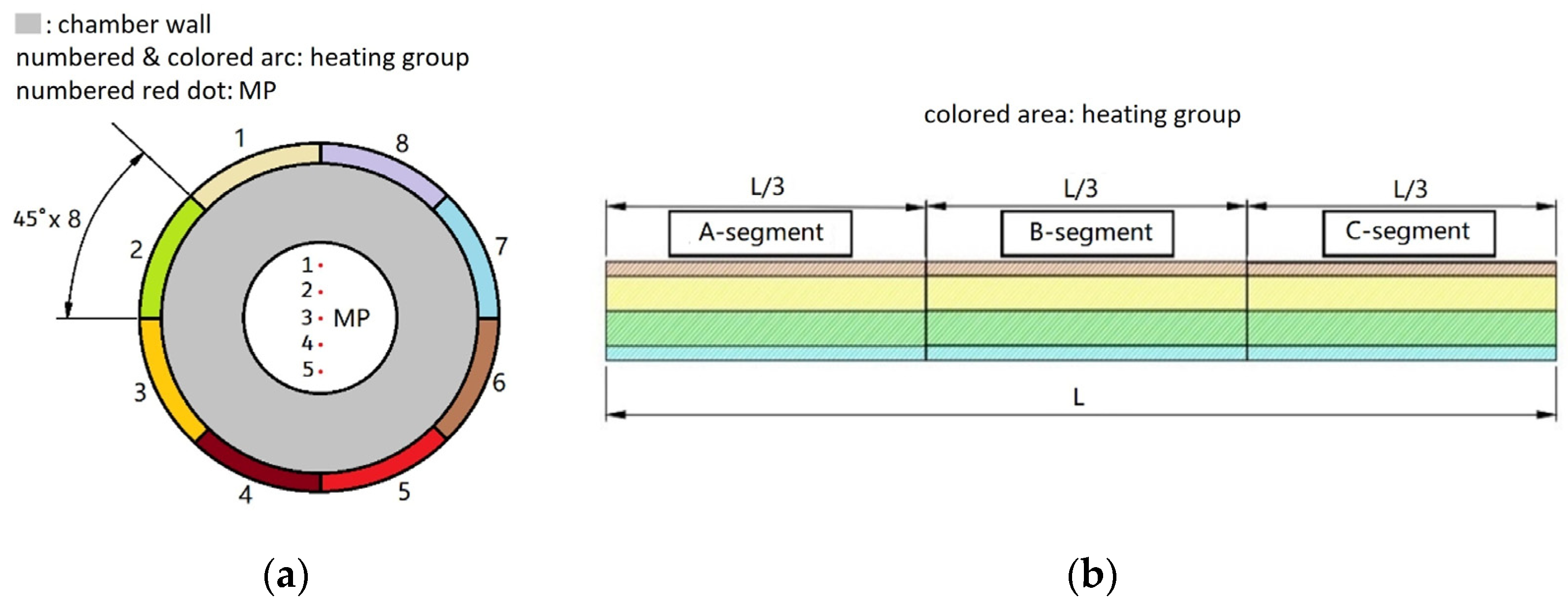
6.1. Study on Uniformity of Electric Heating Temperature Field

The non-uniformity of the internal temperature field of a horizontal cylindrical chamber can be presented by several temperatures at different heights on the cross section of the chamber [29]. As shown in Figure 9, in order to improve the uniformity of the temperature field, we divide the whole electric heating device covering the external surface of a chamber into 3 segments along the axial direction, and 8 groups along the circumferential direction, so there are 24 heating pieces in total. To monitor temperatures at different heights, five temperature-monitoring points (MPs) are uniformly distributed along the vertical diameter in the chamber.

Figure 9. Segmented and grouped heating method; (a) 8 heating groups; (b) 3 heating segments.

A variable UI defined by Equation (11) is used as the temperature field uniformity index, being obtained by recording the temperatures of m MPs at n time points during P temperature control experiments with different target temperatures.

$$UI=\frac{1}{P}{\displaystyle \sum }_{k=1}^P\underset{1\le i\le n}{min}\left(1-\frac{s_k^i}{{\overline{T}}_k^i}\right)$$

(11)

in which,

$$\begin{gathered} s_k^i=\sqrt{\frac{{\sum }_{j=1}^m{\left(T_{jk}^i-{\overline{T}}_k^i\right)}^2}{m-1}} \\ {\overline{T}}_k^i=\frac{{\sum }_{j=1}^m{T}_{jk}^i}{m} \end{gathered}$$

where $T_{jk}^i$ is the temperature of the jth MP at time i in the kth temperature control experiment, ${\overline{T}}_k^i$ represents the average temperature of m MPs at time i in the kth experiment, and $s_k^i$ is the standard deviation of temperatures of m MPs at time i in the kth experiment.

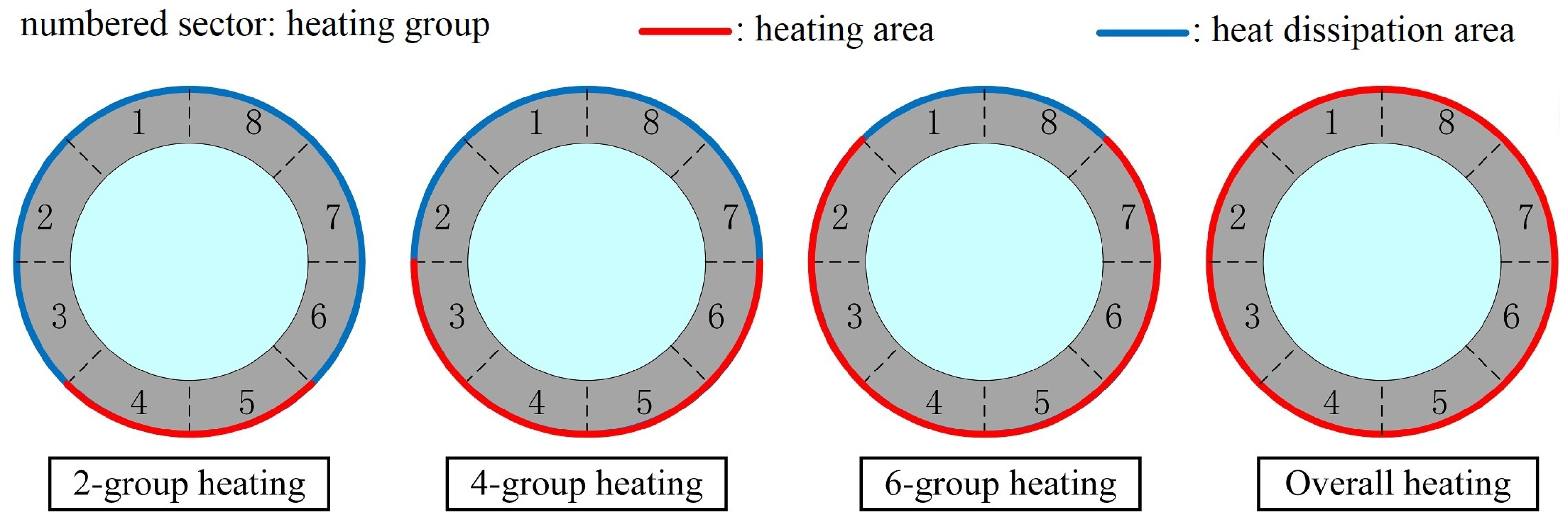
6.2. Simulation of Electric Heating Temperature Field

The simulation model takes 25 °C as the initial temperature, the temperature of MP 3 as the reference, and the chamber wall as the heat source. According to whether heating is on or off, the boundary condition of the chamber wall is set as heat flow density [30] or natural convection heat transfer.

As shown in Figure 10, four heating modes are simulated. The target temperature T_t is set from 40 °C to 80 °C at an interval of 10 °C, and the heat flow density of 5 kW/m² is used as the boundary condition.

Figure 10. Four heating modes.

Figure 11 shows the temperature simulation curve with T_t = 60 °C. When the temperature of MP 3 is lower than T_t, start heating immediately, and stop when higher than T_t. The temperature control process is divided into three stages, i.e., heating stage, overshoot cooling stage and steady state. The error of the steady state is controlled within ±0.5 °C. The UIs of heating stage and steady state under different heating modes and the durations of cooling stage are shown in Table 2.

Figure 11. The temperature simulation curves.

Table 2. UIs in different stages and cooling durations of different heating modes.

Heating Mode	UI/%		Duration of Cooling Stage/min
	Heating Stage	Steady State
2-group	98.29	99.66	27.88
4-group	97.36	99.71	44.52
6-group	93.24	99.51	55.21
overall	84.75	98.96	98.26

From the simulation results, it can be seen that:

• In the heating stage, the less the heating groups, the better the temperature uniformity. The temperature field uniformity of the 2-group heating mode is the best, while that of the overall heating mode is the worst. In the steady state, the uniformities of temperature field of different heating modes are all improved, and the 4-group heating mode has the best result;
• The more the heating groups, the longer the cooling duration is;
• 4-group heating mode has a better overall performance in terms of temperature uniformity and cooling speed.

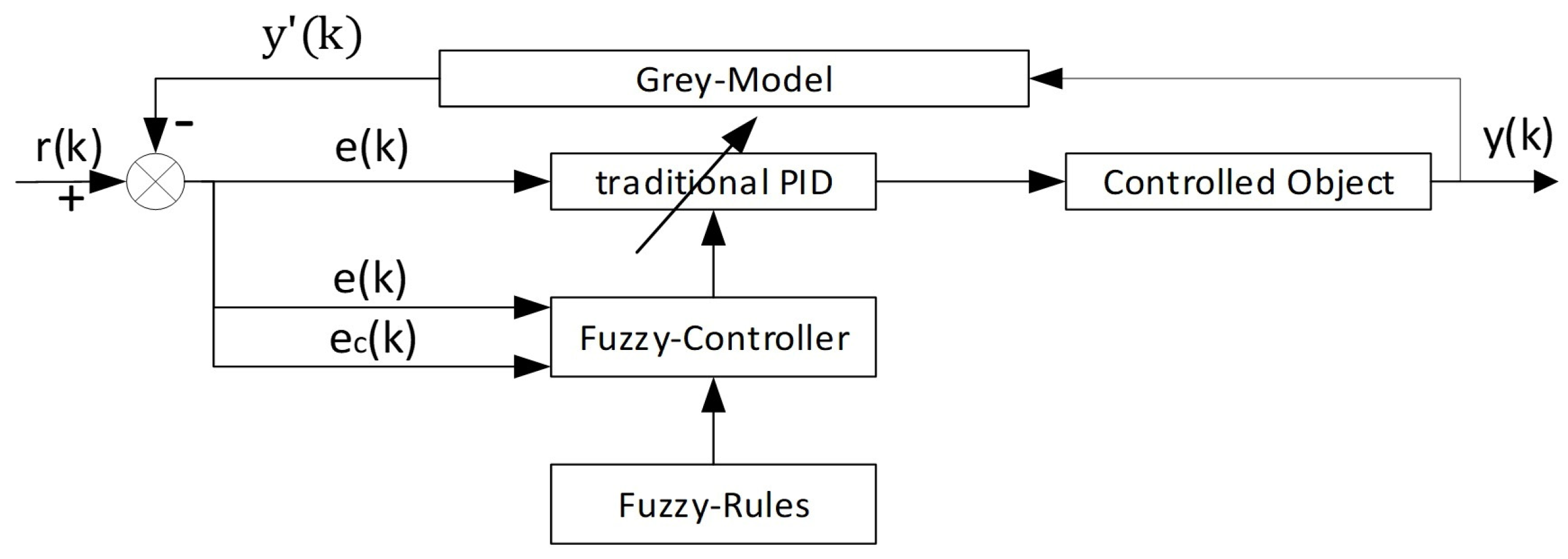
6.3. Fuzzy PID Temperature Control Based on Grey Prediction Model

The temperature control system of the SERCT is a nonlinear, time-varying, large time delay system. Conventional PID control and fuzzy PID control can hardly avoid the overshoot and ensure the stability of the system. In our research a grey prediction model is adopted, which replaces the input of the PID method with the prediction value instead of the feedback value to reduce the overshoot and improve the stability of the system [31,32].

6.3.1. Grey Prediction Model

GM(1,1) model is adopted for grey prediction. GM(1,1) model establishes a first-order ordinary differential equation (ODE) by the accumulation sequence of the original data sequence, as shown in Equation (12), then solves the ODE and obtain the prediction values by inverse accumulated generating operation(IAGO) on the solution sequence.

$$\frac{d{X}^{\left(1\right)}\left(t\right)}{dt}+a{X}^{\left(1\right)}\left(t\right)=b$$

(12)

where $X^{\left(1\right)}=\left\{x^{\left(1\right)}\left(k\right),\left(k=1,\dots ,n\right)\right\}$ is the accumulation sequence of the original data sequence $X^{\left(0\right)}=\left\{x^{\left(0\right)}\left(k\right),\left(k=1,\dots ,n\right)\right\}$, with $x^{\left(1\right)}\left(k\right)={\sum }_{i=1}^k{x}^{\left(0\right)}\left(i\right),k=1,\cdots ,n$. In this study, the dimension n of the data sequence is fixed as 15.

The solution of the ODE (12) is:

$${\widehat{x}}^{\left(1\right)}\left(k+m\right)=\left[x^{\left(0\right)}\left(1\right)-\frac{b}{a}\right]e^{-a\left(k+m-1\right)}+\frac{b}{a}$$

(13)

And the solution for $X^{\left(0\right)}$ can be obtained by IAGO:

$${\widehat{x}}^{\left(0\right)}\left(k+m\right)=\left[x^{\left(0\right)}\left(1\right)-\frac{b}{a}\right]\left(1-e^a\right)e^{-a\left(k+m-1\right)}$$

(14)

where ${\widehat{x}}^{\left(0\right)}\left(k+m\right)$ is the prediction value at the time point of k + m.

The coefficients a and b in Equation (12) can be calculated by the data sequence. Calculate the weighted nearest neighbor sequence $Z^{\left(1\right)}=\left\{z^{\left(1\right)}\left(k\right),k=2,\cdots ,n\right\}$ of $X^{\left(1\right)}$, with $z^{\left(1\right)}\left(k\right)=\frac{1}{2}{x}^{\left(1\right)}\left(k-1\right)+\frac{1}{2}{x}^{\left(1\right)}\left(k\right)$, then the ODE (12) can be discretized into a difference equation as Equation (15).

$$x^{\left(0\right)}\left(k\right)+a{z}^{\left(1\right)}\left(k\right)=b$$

(15)

Because $X^{\left(0\right)}$ and $Z^{\left(1\right)}$ are given, a and b can be obtained by the least square method.

6.3.2. Grey-Prediction-Based Fuzzy PID Controller

Figure 12 shows the schematic diagram of the controller, in which the inputs of the fuzzy controller are the difference e between the target value r(k) and the result y′(k) calculated by the grey prediction model and its change rate e_c. The outputs of the fuzzy controller are the correction values, i.e., ΔK_p, ΔK_i and ΔK_d, of the PID parameters K_p, K_i and K_d, respectively. The PID parameter tuning is achieved by the following formula:

K_p = K′_p + ΔK_p
K_i = K′_i + ΔK_i
K_d = K′_d + ΔK_d

(16)

where K′_p, K′_i and K′_d are PID parameters before correction.

Figure 12. Schematic diagram of fuzzy PID controller based on grey prediction model.

The fuzzy linguistic variables of temperature control are the same as the fuzzy pressure control. The domain of discourse E of e and EC of e_c, ΔK_p, ΔK_i and ΔK_d, are all [−3, 3]. The main task of the fuzzy controller is to construct inference rules of ΔK_p, ΔK_i and ΔK_d by E and EC, as shown in Table 3. The center-of-gravity method is used for defuzzification.

Table 3. Inference rules of ΔK_p, ΔK_i and ΔK_d.

U (ΔKp/ΔKi/ΔKd)		EC
		NB	NM	NS	ZO	PS	PM	PB
E	NB	PB/NB/PS	PB/NB/NS	PM/NM/NB	PM/NM/NB	PS/NS/NB	ZO/ZO/NM	ZO/ZO/PS
	NM	PB/NB/PS	PB/NB/NS	PM/NM/NB	PS/NS/NM	PS/NS/NM	ZO/ZO/NS	NS/ZO/ZO
	NS	PM/NB/ZO	PM/NM/NS	PM/NS/NM	PS/NS/NM	ZO/ZO/NS	NS/PS/NS	NS/PS/ZO
	ZO	PM/NM/ZO	PM/NM/NS	PS/NS/NS	ZO/ZO/NS	NS/PS/NS	NM/PM/NS	NM/PM/ZO
	PS	PS/NM/ZO	PS/NS/ZO	ZO/ZO/ZO	NS/PS/ZO	NS/PS/ZO	NM/PM/ZO	NM/PB/ZO
	PM	PS/ZO/PM	ZO/ZO/PS	NS/PS/PS	NM/PS/PS	NM/PM/PS	NM/PB/PS	NB/PB/PS
	PB	ZO/ZO/PB	ZO/ZO/PM	NM/PS/PM	NM/PM/PM	NM/PM/PS	NB/PB/PS	NB/PB/PS

7. Experiment Results and Discussion

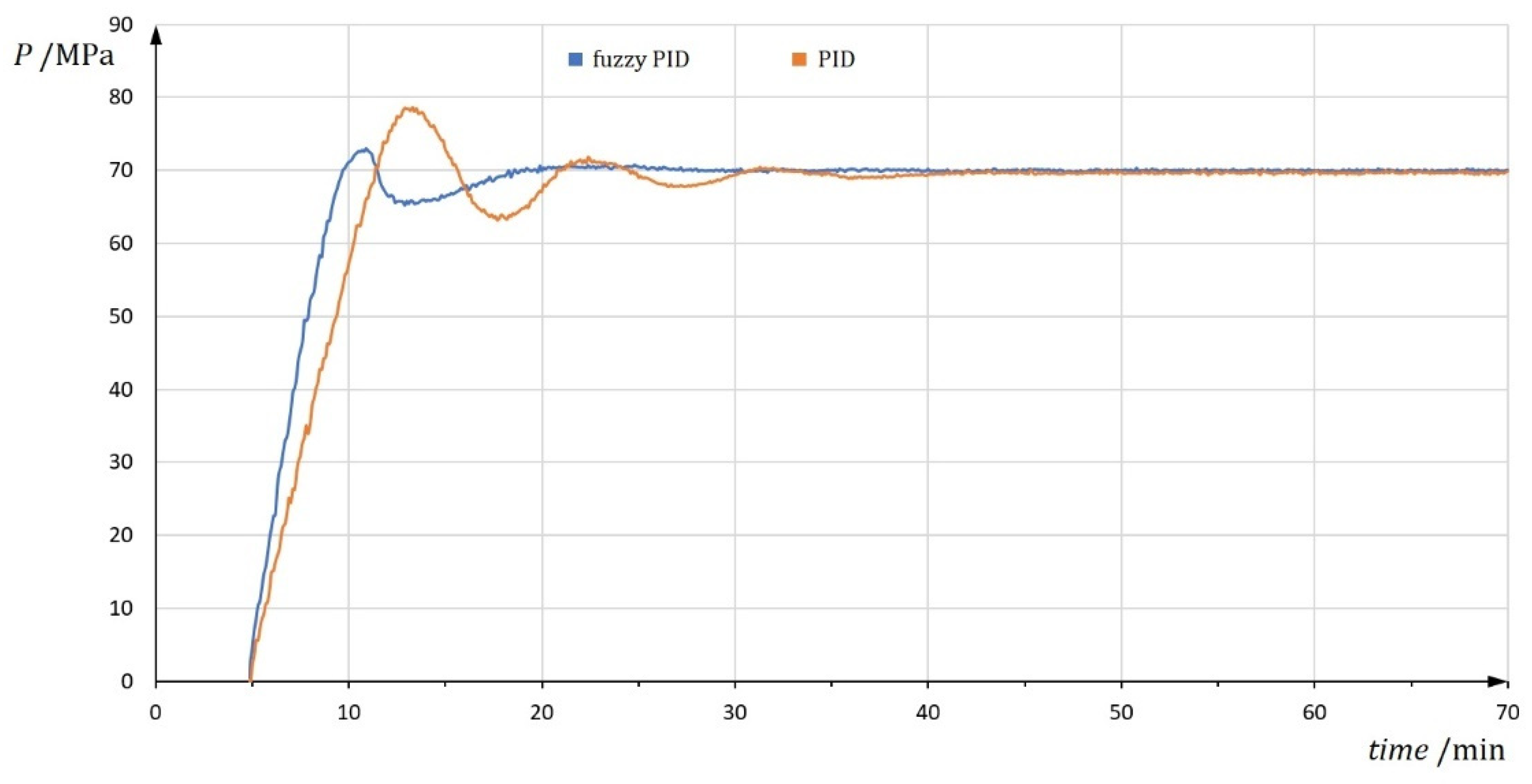
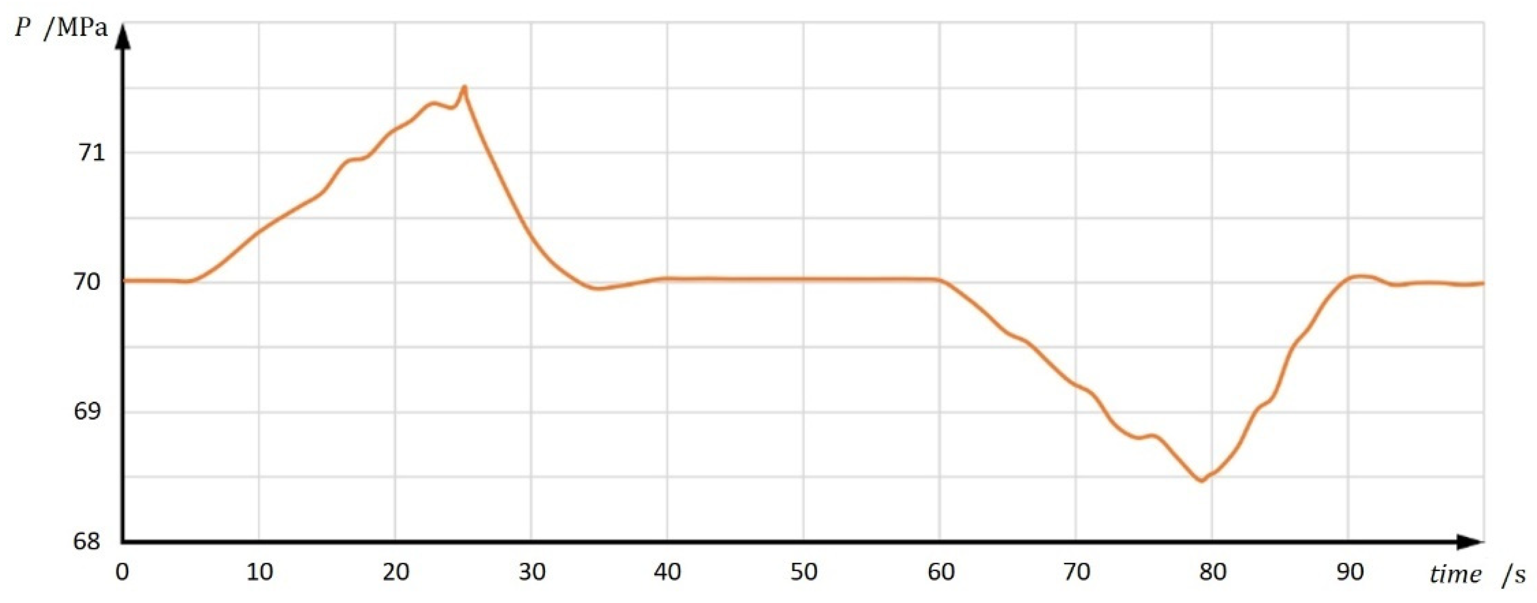
7.1. Experiment of the Fuzzy-PID Dual Mode Pressure Control

In all pressure experiments, water was distilled and boiled to minimize the impact of impurities and dissolved air in the water. Figure 13 shows the results of 70 MPa pressure test on the storage chamber of the SERCD. The internal volume of the chamber is 35.33 L. The maximum output pressure of the booster valve is 425 MPa with the flow per stroke being 3.93 mL. The simple PID control and the fuzzy-PID dual mode control were tested. The steady-state errors of both methods were less than F.S. 1%. When the PID parameters K_p, K_i and K_d of both methods were 300, 12 and 1.5, it can be seen that compared with the simple PID control, the response speed of the fuzzy-PID dual mode control was faster and the overshoot was smaller.

Figure 13. The results of 70 MPa pressure test on the storage chamber.

7.2. Experiment of the Uniformity of Temperature Field

In the heating experiment, the silicone heating tapes were wound outside the storage chamber and covered with insulating cotton for heat insulation, as shown in Figure 14. The power supply was DC 24 V for each heating group. The heating power was 835 W for each two groups. Each heating group could be powered on or off by a solid-state relay. Five PT100 temperature sensors were mounted on the positions MP1~MP5 as shown in Figure 9a.

Figure 14. The heating experiment setup.

The experimental results are shown in Table 4. It can be seen that the 2-group and the 4-group heating modes had good temperature uniformity (>99%) in the heating stage and the steady state, which verifies the simulation results. The duration of heating stage of the 2-group heating mode was twice that of the 4-group heating mode, with the overall time to reach the steady state being the longest and the heating efficiency being the worst. The 4-group heating mode had the best temperature uniformity (99.23%) in the steady state. Therefore, the 4-group heating mode was selected as the preferred heating mode of the SERCT.

Table 4. Experimental results of temperature uniformity and durations of different heating modes.

Heating Mode	UI/%		Duration/min
	Heating Stage	Steady State	Heating Stage	Cooling Stage
2-group	99.20	99.12	90.23	23.54
4-group	99.07	99.23	43.50	44.52
6-group	98.14	98.96	30.24	71.15
overall	91.30	98.46	32.23	79.71

7.3. Experiment of the Fuzzy PID Temperature Control Based on Grey Prediction Model

Figure 15 shows the temperature curves of the storage chamber using the fuzzy PID control and the grey-prediction-based fuzzy PID control with the target temperature of 85 °C. te MPa, tempB and tempC are the temperatures of A-segment, B-segment and C-segment of the chamber, respectively. In the experiment the 4-group heating mode was adopted. Table 5 shows the experiment results of 75 °C, 85 °C and 95 °C. It can be seen that compared with the fuzzy PID control, the overshoot and steady-state errors of the grey-prediction-based fuzzy PID control were relatively lower, with the steady-state errors less than ±0.13% and the overshoots less than 0.22%.

Figure 15. Temperature curves of heating experiments of 85 °C; (a) Fuzzy PID control; (b) Grey-prediction-based Fuzzy PID Control.

Table 5. Comparison of experimental results.

Target Temp.	Performance	Fuzzy PID			Grey Prediction Based Fuzzy PID
		Sect. A	Sect. B	Sect. C	Sect. A	Sect. B	Sect. C
75 °C	Overshoot/%	0.14	0.25	0.48	0.07	0.10	0.13
	Steady-state error/°C	−0.20	0.28	0.17	0.10	−0.11	0.12
85 °C	Overshoot/%	0.19	0.19	0.14	0.09	0.14	0.18
	Steady-state error/°C	0.29	0.25	0.13	0.13	−0.10	−0.10
95 °C	Overshoot/%	0.28	0.29	0.20	0.17	0.22	0.10
	Steady-state error/°C	0.33	−0.26	0.14	0.13	0.12	0.13

7.4. Experiment of the Temperature and Pressure Decoupling Control

In the process of initial environment reconstruction, the water in the storage chamber was heated from 25 °C and 0.1 MPa to 95 °C and 70 MPa. As shown in Figure 16, the decoupling control path ABCDE consists of four steps:

Figure 16. The planning of the P-T decoupling control path.

Step 1. Iso–thermal pressurizing from A (25 °C, 0.1 MPa) to B (25 °C, 10 MPa). During the heating process from 25 °C to 95 °C, the water pressure reduction caused by the expansion of the chamber is about 6 MPa. Therefore, in order to reduce the possible water supplement operation during the reconstruction, the system was pressurized to 10 MPa in advance.

Step 2. Iso–mass heating from B (25 °C, 10 MPa) to C (60 °C, 40.3 MPa).

Step 3. Iso–thermal depressurizing from C(60 °C, 40.3 MPa) to D(60 °C, 22.7 MPa).

Step 4. Iso–mass heating from D (60 °C, 22.7 MPa) to E (95 °C, 70 MPa).

Where C and D were planned by B and E, respectively, according to Equation (7).

Figure 17a shows the temperature and the pressure curves during the process and Figure 17b shows the P-T curve, in which B′, C′, D′ and E′ were the real values of target points B, C, D and E, respectively. When the system was stable at points B′, C′ and D′, the temperature and pressure values were B′(25 °C, 10.1 MPa), C′(60.2 °C, 38.2 MPa), D′(60.2 °C, 22.6 MPa) and E′(95.2 °C, 68.4 MPa), respectively. It can be seen that there were errors on the control points. Besides the accuracy of the control algorithm, there were many others factors that might cause these steady-state errors; for example, the physical characteristics of water might change under different pressures and temperatures, the non-uniformity of the temperature field in the chamber might have an impact on the relationship between temperature and pressure and the actual thermal deformation of the chamber might be different from the theoretical one. To improve the accuracy of the system, after the reconstruction process reached point E′, an iso–thermal pressure fine-tuning was carried out to ensure that the system is stable at E(94.9 °C, 70.1 MPa).

Figure 17. Results of the experiment of initial environment reconstruction. (a) The temperature curve and the pressure curve; (b) The temperature–pressure curve.

In the process of P-T preservation, the pressure and temperature changes during the push rod pushing out and retracting were examined. With the internal volume of the storage chamber being 35.33 L and the diameter of the push rod being 50 mm, according to Equation (9) when the push rod moves 10 mm each time, the pressure fluctuation can be controlled within 1.5 MPa, less than 2%. The speed of the push rod was 0.5 mm/s. The test steps were as follows: (1) let the push rod move out by 10 mm; (2) stopped the push rod and waited till the system got stable; (3) then pulled the push rod back by 10 mm; (4) stopped the push rod and waited till the system got stable again. The test was repeated 10 times. Figure 18 shows the curve obtained by averaging the pressure values of the 10 tests at 85 °C. It can be seen that the pressure fluctuation was controlled within 1.5 MPa.

Figure 18. The pressure curve during the push rod movement.

There were always temperature fluctuations when the push rod moved, but these fluctuations had no obvious regularity. This might be related to the disturbance of the push rod movement to the uniformity of the temperature field, or to the change of the temperature conduction characteristics in the chamber due to the movement of the metal push rod. However, because of the preheating mode adopted by the SERCT, even in the process of water replenishment, the water temperature in the chamber did not change significantly, and the temperature errors were controlled within 1%.

8. Conclusions

In this paper, the structure of the SERCT and the principle of its two-layer temperature and pressure control are given. A P-T interpolation decoupling control algorithm based on the iso–density P-T curves of water is proposed for its high-temperature and high-pressure coupling control problem. The control path is divided into two kinds of independent interpolation paths, namely, iso–thermal pressure control and iso–mass temperature control. The decoupled pressure control adopts fuzzy PID dual mode control, which reduces the dynamic response time and the overshoot. The phenomenon of temperature stratification of water in the chamber during the heating process is studied, and a three-segment eight-group electric heating method is proposed to improve the uniformity of the temperature field inside the chamber. In view of the low cooling efficiency of the electric heating method, the fuzzy PID temperature control algorithm based on the grey prediction model is adopted in this study to achieve a very small overshoot and low static error.

Future works mainly focus on further improving the capacity of the SERCT to 140 MPa and 150 °C, and studying the P-T control under the environment of such high temperature and ultra-high pressure, exploring other heating methods that can achieve better temperature uniformity and higher heating and cooling efficiency at the same time.

References

1. Lu, Y.C.; He, Z.Q.; Wang, Y.W.; Dai, Z.X.; Wang, Z.J. Mining-induced mechanics behavior in the deep mine with an overkilometer depth. J. China Coal Soc. 2019, 44, 1326–1336. [Google Scholar]
2. Xie, H.P.; Li, C.B.; Gao, M.Z.; Zhang, R.; Gao, F.; Zhu, J.B. Conceptualization and preliminary research on deep in situ rock mechanics. Chin. J. Rock Mech. Eng. 2021, 40, 217–232. [Google Scholar]
3. Zhang, Z.P.; Xie, H.P.; Zhang, R.; Zhang, Z.T.; Gao, M.Z.; Jia, Z.Q.; Xie, J. Deformation damage and energy evolution characteristics of coal at different depths. Rock Mech. Rock Eng. 2019, 52, 1491–1503. [Google Scholar] [CrossRef]
4. Xie, H.P.; Gao, M.Z.; Zhang, R.; Chen, L.; Liu, T.; Li, C.B.; Li, C.; He, Z.Q. Study on concept and progress of in situ fidelity coring of deep rocks. Chin. J. Rock Mech. Eng. 2020, 39, 865–876. [Google Scholar]
5. Li, C. Reliability Analysis of Deep-Sea Ultra-High Pressure Environment Simulation System; SOA: Beijing, China, 2013. [Google Scholar]
6. Zhang, J.N. Study on Acoustic Testing System for Pressure Environment Simulation of Seabed Sediment. Master’s Thesis, Guangdong University of Technology, Guangzhou, China, 2021. [Google Scholar]
7. Molfino, P.; Nervi, M.; Rossi, M.; Malgarotti, S.; Odasso, A. Design and development of a module for the construction of reversible HVDC submarine deep-water sea electrodes. IEEE Trans. Power Deliv. 2017, 32, 1682–1687. [Google Scholar] [CrossRef]
8. Gauthey, J.R.; Ventriglio, F.J. Naval Ship Systems Command Research and Development Program on Pollution Abatement; American Society of Mechanical Engineers: New York, NY, USA, 1973; Volume 95, p. 69. [Google Scholar]
9. McInroy, J.E.; Neat, G.W.; O’Brien, J.F. A robotic approach to fault-tolerant, precision pointing. IEEE Robot. Autom. Mag. 1999, 6, 24–31. [Google Scholar] [CrossRef]
10. AMSTEC. Facilities and Equipment in Yokosuka Headquarters. 2003. Available online: https://www.jamstec.go.jp/e/about/equipment/yokosuka/chugata_kouatsu_jikken.html (accessed on 22 May 2023).
11. Qing, X. Design and Finite Element Analysis of a Super High Pressure Cylinder. Master’s Thesis, Sichuan University, Chengdu, Chian, 2017; pp. 3–40. [Google Scholar]
12. Wang, W.T. Study on Pressure Retaining Transfer Device for Deep-Sea Sediments. Master’s Thesis, Zhejiang University, Hangzhou, China, 2015. [Google Scholar]
13. Zeng, R.Y.; Chan, Z.H. Progress in research and development techniques on deep sea microorganism resource. Chin. Bull. Life Sci. 2012, 24, 991–996. [Google Scholar]
14. Ross, P.S.; Bourke, A.; Fresia, B. A multi-sensor logger for rock cores: Methodology and preliminary results from the Matagami mining camp, Canada. Ore Geol. Rev. 2013, 53, 93–111. [Google Scholar] [CrossRef]
15. Schultheiss, P.J.; Francis, T.J.G.; Holland, M.; Roberts, J.A.; Amann, H.; Thjunjoto, R.J.; Parkes, R.J.; Martin, D.; Rothfuss, M.; Tyunder, F.; et al. Pressure Coring, Logging and Subsampling with the Hyacinth System; Geological Society: London, UK, 2006; Volume 267, pp. 151–163. [Google Scholar]
16. Liu, J.B. Study on Pressure Maintaining System of Gas Hydrate Transfer Device. Master’s Thesis, Zhejiang University, Hangzhou, China, 2016. [Google Scholar]
17. Liu, H.; Lee, J.C.; Li, B.R. High precision pressure control of a pneumatic chamber using a hybrid fuzzy PID controller. Int. J. Precis. Eng. Manuf. 2007, 8, 8–13. [Google Scholar]
18. Yu, L.; Lim, J.G.; Fei, S.M. An improved single neuron self-adaptive PID control scheme of superheated steam temperature control system. Int. J. Syst. Control. Inf. Process. 2017, 2, 1–13. [Google Scholar] [CrossRef]
19. Chew, I.M.; Wong, F.; Bono, A.; Nan, D.J.; Wong, K.I. Genetic algorithm optimization analysis for temperature control system using cascade control loop model. Int. J. Comput. Digit. Syst. 2020, 9, 119–128. [Google Scholar]
20. Shakeri, E.; Latif-Shabgahi, G.; Abharian, A.E. Design of an intelligent stochastic model predictive controller for a continuous stirred tank reactor through a Fokker-Planck observer. Trans. Inst. Meas. Control. 2018, 40, 3010–3022. [Google Scholar] [CrossRef]
21. Shi, H.Y.; Li, P.; Wang, L.M.; Su, C.L.; Yu, J.X.; Cao, J.T. Delay-range-dependent robust constrained model predictive control for industrial processes with uncertainties and unknown disturbances. Complexity 2019, 2019, 2152014. [Google Scholar] [CrossRef]
22. Aguilar-López, R.; Mata-Machuca, J.L.; Godinez-Cantillo, V. A tito control strategy to increase productivity in uncertain exothermic continuous chemical reactors. Processes 2021, 9, 873. [Google Scholar] [CrossRef]
23. Dorigo, M.; Maniezzo, V.; Colorni, A. Ant system: Optimization by a colony of cooperating agents. IEEE Trans. Syst. Man Cybern. Part B 1996, 26, 29–41. [Google Scholar] [CrossRef] [PubMed]
24. Wang, Y.B.; Chen, W.N.; Wang, X.D.; Wang, D.C. Overview of Pressure Control System Based on PID Algorithm. Proc. First Pearl River Sci. Assoc. Forum 2011, 128–132. [Google Scholar]
25. Qian, X.; Huang, K.J.; Jia, S.K.; Chen, H.S.; Yuan, Y.; Zhang, L.; Wang, S.F. Temperature difference control and pressure-compensated temperature difference control for four-product extended Petlyuk dividing-wall columns. Chem. Eng. Res. Des. 2019, 146, 263–276. [Google Scholar] [CrossRef]
26. Pan, H.; Wu, X.; Qiu, J.; He, G.C.; Ling, H. Pressure compensated temperature control of Kaibel divided-Wall column. Chem. Eng. Sci. 2019, 203, 321–332. [Google Scholar] [CrossRef]
27. Zheng, Y.G.; Liu, M.; Wu, H.; Wang, J. Temperature and Pressure Dynamic Control for the Aircraft Engine Bleed Air Simulation Test Using the LPID Controller. Aerospace 2021, 8, 367. [Google Scholar] [CrossRef]
28. The International Association for the Properties of Water and Steam, IAPWS R6-95(2018), Revised Release on the IAPWS Formulation 1995 for the Thermodynamic Properties of Ordinary Water Substance for General and Scientific Use, 2018. Available online: http://www.iapws.org/relguide/IAPWS-95.html (accessed on 22 May 2023).
29. Li, X.J.; Wu, M.W.; Wan, L.H.; Wu, J.J.; Zhang, H.Y. Simulation and experimental study of uniformity of temperature field of water by electric heating. J. Shenzhen Univ. Sci. Eng. 2022, 39, 314–323. [Google Scholar] [CrossRef]
30. Ghani, A.A.; Farid, M.M. Numerical simulation of solid-liquid food mixture in a high pressure processing unit using computational fluid dynamics. J. Food Eng. 2007, 80, 1031–1420. [Google Scholar] [CrossRef]
31. Zhang, Y.B.; Wei, Z.Y.; Lin, Q.Y.; Zhang, L.; Xu, J. MBD of gray prediction fuzzy-PID irrigation control technology. Desalination Water Treat. 2018, 110, 328–336. [Google Scholar] [CrossRef]
32. Kayacan, E.; Kaynak, O. An adaptive gray PID-type fuzzy controller design for a non-linear liquid level system. Trans. Inst. Meas. Control. 2009, 31, 33–49. [Google Scholar] [CrossRef]
Disclaimer/Publisher’s Note: The statements, opinions and data contained in all publications are solely those of the individual author(s) and contributor(s) and not of MDPI and/or the editor(s). MDPI and/or the editor(s) disclaim responsibility for any injury to people or property resulting from any ideas, methods, instructions or products referred to in the content.
Article Metrics
Citations
Article Access Statistics
Multiple requests from the same IP address are counted as one view.