Review of Anomaly Detection Algorithms for Data Streams

Abstract

With the rapid development of emerging technologies such as self-media, the Internet of Things, and cloud computing, massive data applications are crossing the threshold of the era of real-time analysis and value realization, which makes data streams ubiquitous in all kinds of industries. Therefore, detecting anomalies in such data streams could be very important and full of challenges. For example, in industries such as electricity and finance, data stream anomalies often contain information that can help avoiding risks and support decision making. However, most traditional anomaly detection algorithms rely on acquiring global information about the data, which is hard to apply to stream data scenarios. Currently, the reviews of the algorithm in the field of anomaly detection, both domestically and internationally, tend to focus on the exposition of anomaly detection algorithms in static data environments, while lacking in the induction and analysis of anomaly detection algorithms in the context of streaming data. As a result, unlike the existing literature reviews, this review provides the current mainstream anomaly detection algorithms in data streaming scenarios and categorizes them into three types on the basis of their fundamental principles: (1) based on offline learning; (2) based on semi-online learning; (3) based on online learning. This review discusses the current state of research on data stream anomaly detection and studies the key issues in various algorithms for detecting anomalies in data streams on the basis of concise summarization. Moreover, the review conducts a detailed comparison of the pros and cons of the algorithms. Finally, the future challenges in the field are analyzed, and future research directions are proposed.

1. Introduction

Data streams have become a vital source of big data [1,2,3,4]. With the advent of the big data era, data streams are generated in various industries as the predominant form of business data. Consequently, data streams have gradually become a research focus in the fields of data mining and information security.

Anomaly detection, as an important branch of data mining, aims to identify data patterns that deviate from expected behaviors within data streams. These anomalous patterns often contain crucial information, which is commonly leveraged to assist decision-making processes. Therefore, data stream anomaly detection has emerged as a critical task in data analysis and security domains, finding widespread application in the following scenarios:

• Financial risk management: Data stream anomaly detection is utilized for identifying, analyzing, and predicting credit card fraud, insurance scams, and other fraudulent activities in banking card transactions [5]. Commercial banks also employ data stream anomaly detection methods to analyze real-time exchange rate anomalies, thus preventing substantial financial losses to banks and customers.
• Power grid operations: Data stream anomaly detection is commonly employed to detect anomalies in power scheduling data, ensuring the secure operation of power systems [6].
• Healthcare applications: Data stream anomaly detection is frequently used for detecting abnormal patterns in medical image data, pulse data, blood pressure data, and other streaming healthcare data. These anomalies serve as fundamental indicators for diagnosing abnormal human conditions [7].
• Computer network security: Data stream anomaly detection is typically employed to detect intrusions that violate security policies [8].

Compared to static data, data stream anomaly detection faces unprecedented challenges [9] due to the following characteristics:

• Continuous data influx: Data arrives in a continuous stream, making it costly to perform multiple scans or store all the data. Therefore, algorithms/models are required to operate in resource-constrained environments.
• High data generation rates: Due to this characteristic, relevant algorithms must possess real-time processing and analysis capabilities.
• Data stream dynamics and evolution: Anomalous behaviors in data streams can change over time, rendering traditional static anomaly detection methods inadequate. Data stream anomaly detection algorithms need to be adaptive, capable of automatically learning and adjusting to changes within the data stream, thereby maintaining efficient anomaly detection performance.

Given the challenges in data stream anomaly detection, the significance of effective algorithms becomes particularly prominent.

Presently, there are numerous surveys on anomaly detection algorithms. However, the existing literature [10,11,12,13,14] primarily focuses on static data environments and lacks reference value for data stream environments. While some studies [15,16] extensively survey anomaly detection algorithms for time series data, they allocate limited space to data stream anomaly detection, thereby offering limited insights into this specific field. Another study [17] primarily focuses on the performance of data stream anomaly detection algorithms in forest fire prediction, restricting its scope to a specific scenario and lacking a systematic classification approach. Additionally, a recent survey [18] explores high-dimensional data stream anomaly detection algorithms in terms of efficiency and effectiveness and proposes a new classification method for high-dimensional data stream anomaly detection. However, it fails to describe relevant content on non-high-dimensional data stream anomaly detection algorithms.

In summary, existing surveys in the anomaly detection field have limited reference value for data stream environments. Furthermore, to the best of our knowledge, there is currently no systematic classification and review of data stream anomaly detection algorithms in the field of machine learning. Therefore, this paper systematically organizes and analyzes relevant literature, providing a comprehensive review of recent research in this area.

This paper proposes an innovative classification method for data stream anomaly detection algorithms, as shown in Figure 1. This classification method allows for a scientific and systematic categorization of existing and future data stream anomaly detection algorithms. Furthermore, on the basis of the proposed classification system for data stream anomaly detection algorithms, this paper provides a detailed comparison and summary of the advantages and limitations of different algorithm categories, covering major categories and subcategories. This can assist readers in selecting appropriate data stream anomaly detection algorithm categories for specific environments.

The paper divides data stream anomaly detection algorithms into three major categories: Based on offline learning, based on semi-online learning, and based on online learning. The comparative advantages and disadvantages of these three algorithm categories are presented in

Table 1. Overview of anomaly detection algorithms for data streams.

Algorithm Type	Algorithm Name and Reference	Advantages	Disadvantages
Based on offline learning	K-means [19]; KNN [20]; LOF [21]; OCSVM [22]; IForest [23]; RS-Hash [24]; DeepAnT [25]; SISVAE [26]; GANomaly [27]; AEAD [28]	Using all available historical data for model training, therefore achieving better performance in anomaly detection.	Cannot handle new data patterns; cannot handle real-time streaming data; requires manual tuning.
Based on semi-online learning	MiLOF [29]; NETS [30]; EC-SVM [31]; Storm [32]; Storm1, 2, 3 [33]; MCOD [34,35]; pMCOD [36]; DILOF [37]; CODS [38]; iForestASD [39]; LSHiforest [40];	Compared with offline learning algorithms, it can adapt to changes in data distribution and save computation time; compared with online learning algorithms, it can use more complex models and algorithms.	The performance of the algorithm depends on the segmentation method of the data stream and the update frequency of the algorithm model.
Based on online learning	osPCA [41]; OSHULL [42]; The deterministic flow update algorithm [43]; The stochastic stream update algorithm [43]; A framework of virtual war room and matrix sketch-based streaming anomaly detection [44]; VFDT [45]; CVFDT [46]; HAT [47]; EFDT [48]; GAHT [49]; ADA [50]; DAGMM [51]; ARCUS [52]; S-DPS [53]	Real-time and fast detection of anomalies; ability to adapt to changes in data distribution; low storage cost.	The algorithm is simple but less accurate, and there is instability in real-time processing.

, while the detailed advantages and disadvantages of subcategories within each branch are discussed in Section 3, Section 4 and Section 5 of this paper.

The organization of the paper is as follows: In Section 1, the background and contributions of this paper are introduced. Section 2 presents the relevant concepts of data stream anomaly detection. Section 3, Section 4 and Section 5 offer a comprehensive analysis and summary of data stream anomaly detection algorithms in each subcategory: offline learning, semi-online learning, and online learning approaches. The discussion includes a comparative examination of their advantages and disadvantages. Section 6 discusses future research work for the authors, challenges that still exist in the field of data stream anomaly detection, and promising research directions. Finally, in Section 7, the paper concludes and provides an outlook for future work.

2. Data Stream Anomaly Detection: Concepts

Anomaly detection is the process of detecting events that violate security by monitoring system audit records for abnormal usage. A data stream is a sequence of numerous, continuous, real-time, and ordered data items. Anomaly detection based on data streams, which is the main focus of this paper, involves using data streams as input objects for anomaly detection operations.

2.1. Data Streams

Data streams can be seen as data sequences composed of different data items at different times. If t represents any moment in time and x represents the data item at time t, then the data stream can be represented as x1, x2, …, xn. The length of a data stream is the total number of data items it contains. Data streams have the following characteristics:

• Data streams are fluid and fast. Fluid means that new data flows in every moment, while fast means that data streams require timely and effective processing, which can be a heavy burden for computers.
• Data streams have temporal properties. Data streams have a temporal sequence, and we can only access data in the data stream in order.
• Data streams are single pass. Due to the temporal nature of the data and the limitation of device storage space, data items in a data stream can usually only be processed once. This also means that the system cannot retain complete information on all data items.
• Data streams have a certain degree of mutation. The data in a data stream may undergo mutation at a certain point due to external factors, resulting in a significant difference compared to the data before mutation. Mutated data streams may cause errors and inaccuracies in research, which can pose significant challenges for researchers [54].

2.2. Anomaly Detection

An anomaly typically refers to a pattern that deviates from the expected one, where data under this pattern cannot satisfy our definition of the normal data features. Therefore, the process of anomaly detection is to find data under this pattern. As shown in Figure 2 [55], in a two-dimensional dataset, N₁ and N₂, normal data are divided into two areas, and most of the data belong to these two areas. However, some scattered data points that are far from these areas, such as O₁, O₂, O₃, and points in the set of points that are far away from the areas can be considered as anomalous data.

In anomaly detection, the most effective way is to define the features or behaviors of normal data and then determine whether the upcoming unknown data objects are within the range of these defined features or behaviors. If not, the data are defined as anomalous.

3. Data Stream Anomaly Detection Algorithm Based on Offline Learning

The data stream anomaly detection algorithm based on offline learning refers to the use of a certain amount of historical data to train a model before the data stream starts to transmit, obtaining a model that can handle data streams. During the training process, the algorithm uses the entire dataset, so traditional batch processing algorithms can be used. The advantage of this type of algorithm is that it can use a large number of resources for training, thereby achieving high detection accuracy. However, the disadvantage is that it requires a lot of time and computing resources for large-scale streaming data, making it unsuitable for real-time applications. Therefore, this section only introduces several classic offline algorithms and does not summarize related algorithms in depth.

This section introduces four types of offline learning-based data stream anomaly detection algorithms: data stream anomaly detection algorithms based on similarity of data distribution, including LOF (Local Outlier Factor), k-means, and KNN (K-Nearest Neighbors); based on classification principle data stream anomaly detection algorithms such as OCSVM (One-Class Support Vector Machines); data stream anomaly detection algorithms based on subspace partitioning, including iForest (Isolation Forest) and RS-Hash (Randomized Subspace Hashing); and data stream anomaly detection algorithms based on deep learning, including DeepAnT (deep-learning-based anomaly detection approach), SISVAE (Smoothness-Inducing Sequential Variational Auto-Encoder), GANomaly (Generative Adversarial Network Anomaly Detection), and AEAD (Auto-Encoder Anomaly Detection).

Overall, the pros and cons of offline learning-based algorithms are summarized in

Table 2. Overview of anomaly detection algorithms for data streams.

Algorithm Type	Algorithm Name and Reference	Advantages	Disadvantages
Based on similarity of data distribution	K-means [19]; KNN [20]; LOF [21]	The detection performance is better for data streams with slowly changing distribution characteristics and high interpretability.	The algorithm requires strict assumptions about the data distribution; there is a “curse of dimensionality” problem for high-dimensional data.
Based on classification principle	OCSVM [22]	Strong generalization and high scalability.	Sensitive to noise, prone to false positives; requires labeled anomalies; detection results are limited by the degree of balance between positive and negative samples.
Based on subspace partitioning	IForest [23]; RS-Hash [24]	For high-dimensional data, there is no “curse of dimensionality” issue, and there is no need to select features for anomaly detection.	The detection performance is poor for small sample data; the interpretability is low.
Based on deep learning	DeepAnT [25]; SISVAE [26]; GANomaly [27]; AEAD [28]	It can automatically learn feature representations, avoiding the subjectivity of manually defining features.	Requires a large amount of data and computational resources and has poor interpretability.

.

3.1. Based on Similarity of Data Distribution

The main idea of data stream anomaly detection based on similarity of data distribution is to identify anomalous points by modeling the data distribution. Specifically, such algorithms use distribution characteristics such as location, distance, and density of data points in the data distribution to identify anomalous points.

The k-means algorithm proposed in the literature [19] is a classical clustering method. In the anomaly detection task, the distance between each sample and its corresponding cluster center can be used as a measure of its anomaly degree. When the distance between a new sample point and its corresponding cluster center exceeds a certain threshold, the sample point is considered an anomalous point.

The advantage of the k-means algorithm is its intuitiveness and strong interpretability. However, its disadvantage is that it requires a manual parameter setting, and its detection effectiveness is limited by the shape of the cluster.

The KNN algorithm proposed in the literature [20] is a classical distance-based anomaly detection algorithm. The anomaly detection principle of the KNN algorithm is to calculate the distance between a new data point and all data points in the existing dataset, select the K nearest data points, and treat these K data points as a local subspace. The new data point is then determined to belong to the local subspace by calculating the average distance between these K data points and the new data point. If the average distance between the new data point and the local subspace is greater than a certain threshold, it is considered an anomalous point.

The advantage of the KNN algorithm is its simplicity and sensitivity to outliers. However, its detection effectiveness depends on the parameter K.

The LOF algorithm proposed in the literature [21] is a density-based anomaly detection algorithm. In the LOF algorithm, the distance between each data point and its surrounding data points is first calculated, and the k nearest neighbors of each data point are determined. Then, the local reachability density (LRD) of each data point is calculated, which represents the reciprocal of the average distance between a data point and its k-nearest neighbors. Finally, the local outlier factor (LOF) of each data point is calculated, which represents the average ratio of the LRD of a data point and the LRD of its k-nearest neighbors. If the LOF value of a data point is greater than 1, it is considered an anomalous point.

The advantage of the LOF algorithm is that it does not require prior knowledge, parameter setting, or training. However, its detection effectiveness is limited by the data distribution.

3.2. Based on Classification Principle

Data stream anomaly detection based on the classification principle refers to a class of algorithms that use classification algorithms to judge whether data in a data stream are anomalous. These algorithms typically first train on normal data and then use a classifier to classify new data. If the new data are classified as an abnormal class, it is considered to be anomalous data.

One of the representatives based on classification principal data stream anomaly detection algorithms is the one-class SVM algorithm proposed in [22], which is an anomaly detection algorithm based on SVM (Support Vector Machine) classification. Its principle is to map the normal dataset into a high-dimensional space and find an optimal hyperplane (i.e., separation hyperplane) that makes all normal data points on the same side of this hyperplane, while maximizing the distance to the nearest normal data point from the hyperplane. During the testing phase, new data points are mapped into the high-dimensional space and classified on the basis of their position on the hyperplane. If a data point is outside the hyperplane, it is considered an anomalous data point. Unlike traditional SVM, one-class SVM only trains on normal data and does not use anomalous data for training.

The one-class SVM algorithm can adapt to different data distributions by selecting appropriate kernel functions, and its anomaly detection effectiveness is also limited by the choice of kernel function.

3.3. Based on Subspace Partitioning

The data stream anomaly detection method based on subspace partitioning is an anomaly detection technique based on subspace analysis. Its main idea is to decompose the data stream into multiple subspaces, then apply different anomaly detection algorithms in each subspace, and finally merge all the detection results. This method usually requires selecting appropriate subspace partitioning strategies and anomaly detection algorithms to improve the detection accuracy and efficiency.

The iForest algorithm proposed in [23] is a subspace partitioning-based anomaly detection algorithm. It processes data by constructing a random binary search tree to achieve anomaly detection. In the iForest algorithm, for each data point, it is separated from the dataset by random splitting, and the number of times the data point needs to be separated is calculated. By performing such operations on multiple data points, a series of separation numbers can be obtained, and on the basis of these separation numbers, the anomaly score of each data point can be calculated. The higher the anomaly score, the more likely the data point is an outlier.

The advantage of the iForest algorithm is that it does not require feature selection and can detect anomalies in high-dimensional data streams. The disadvantage of the iForest algorithm is that it performs poorly in detecting small sample datasets.

A fast subspace anomaly detection algorithm called HS-Hash is proposed in [24], which uses random hashing technology to process large-scale data in linear time and discover subspace anomaly points of multidimensional data.

The core idea of the algorithm is to use random hashing mapping to transform the original data into a low-dimensional space to reduce the computational complexity and then search for anomaly points in the low-dimensional space. Specifically, the algorithm is divided into the following steps:

• Data preprocessing: Randomly select some dimensions from the original data to form a random subspace based on the dimensionality of the subspace to be detected.
• Hash mapping: For each vector in the random subspace, use a hash function to map it to a bucket.
• Anomaly point detection: For each bucket, calculate the average value of the vectors in it and use it as the center point of the bucket. Then, calculate the distance between each vector and the center point of the bucket. For vectors with distances exceeding a certain threshold, mark them as anomaly points.
• Return results: Return all the anomaly points as the detection results.

The advantage of this algorithm is that it has linear time complexity, can handle large-scale data, and can also discover subspace anomaly points of multidimensional data. However, since the hash function used is random, its interpretability is relatively weak.

3.4. Based on Deep Learning

The deep-learning-based data stream anomaly detection algorithm is a method of detecting anomalous data from data streams using deep learning models. This algorithm can learn the complex intrinsic rules and feature representations of data, thus effectively detecting abnormal points. When using deep learning models for data stream anomaly detection, data preprocessing, feature extraction, model training, and anomaly detection are typically required.

The DeepAnT algorithm proposed in [25] is a deep learning-based anomaly detection algorithm. Its main principle is to use a deep convolutional neural network (CNN) to model normal data and then use this model to detect abnormal data. The algorithm works as follows:

• Preprocessing: Convert raw data into spectrograms for better convolutional operations.
• Construct a deep convolutional neural network: Use multiple convolutional, pooling, and fully connected layers to construct a deep convolutional neural network for modeling normal data.
• Train the network: Train the network using normal data and use cross-entropy as the loss function.
• Anomaly detection: For new data, input it into the trained network; calculate its reconstruction error; and if the reconstruction error is greater than a certain threshold, mark it as abnormal data.

The advantages of the DeepAnT algorithm are that it can effectively handle non-stationary time-series data, but the disadvantage is that the algorithm requires a large amount of training data and manual tuning.

The SISVAE algorithm proposed in [26] is a deep-learning-based anomaly detection algorithm based on Variational Auto-Encoder (VAE). SISVAE differs from standard VAE by adding a smoothness constraint between the encoder and decoder to better capture long-term dependencies in time series. Meanwhile, SISVAE uses a statistical significance-based evaluation method, calculating the distance between reconstruction error and latent representation and comparing the distance value with normal distribution to detect anomalies.

The advantages of the SISVAE algorithm are that it does not require manual tuning, but the disadvantage is its poor performance in handling multimodal data.

The GANomaly algorithm proposed in [27] is a deep-learning-based anomaly detection algorithm based on Generative Adversarial Network (GAN). It uses a framework consisting of two neural networks, a generator, and a discriminator. The main idea of GANomaly is to use the generator to produce normal data during training while letting the discriminator learn how to distinguish between normal and abnormal data. Later, when a test sample is input, the generator is used to convert it into a representation in the latent space, and the discriminator is used to classify it. If the test sample is classified as abnormal, it is considered an anomaly.

The advantages of the GANomaly algorithm are that it can handle multimodal data, but the disadvantage is that it has poor detection performance on small sample datasets.

The algorithm proposed in [28] presents an anomaly detection method based on the autoencoder principle described in [56]. The algorithm framework in the paper is an anomaly detection approach based on autoencoders. By retraining the intermediate layers of the autoencoder model using limited new data from different devices, the researchers achieved anomaly detection for IoT devices infected with malicious software. The specific algorithm principles are as follows:

• Data preprocessing: The dataset undergoes preprocessing steps such as feature extraction, normalization, and dimensionality reduction to facilitate subsequent model training and testing.
• Autoencoder model construction: A multilayer neural network is built as the autoencoder model. The model consists of an encoder and a decoder. The encoder maps the input data to a hidden representation, while the decoder reconstructs the hidden representation into the original input data.
• Model training: The autoencoder model is trained using data from normal devices as the training set. The training aims to minimize the reconstruction error, which measures the difference between the original input data and the decoder’s output.
• Anomaly detection: The trained autoencoder model is used to detect anomalies in the behavior of unknown devices. If the reconstruction error exceeds a predefined threshold, the device’s behavior is deemed anomalous.
• Transfer learning: For each specific type of device, the intermediate layers are retrained using a dataset from that type of device. This process enables the model to better capture the feature representation of that device type.

Through the aforementioned algorithm steps, the researchers achieved an anomaly detection method based on autoencoders and improved the model’s detection capability through transfer learning. This approach demonstrates practicality and effectiveness in detecting malicious behavior in IoT devices. Its advantages include good scalability and low computational resource requirements. However, the limitations of this algorithm framework lie in its dependence on the quality and accuracy of feature extraction. If the feature extraction method is not suitable for a specific environment or device type, it can impact the algorithm’s performance. Additionally, since the algorithm is trained and tested on existing datasets, it may not effectively handle unknown anomalous behavior.

Combining the findings from Table 2, we summarize the classification of data stream anomaly detection algorithms on the basis of offline learning as follows:

• Algorithms based on similarity of data distribution: The advantage of these algorithms is their simplicity and intuitive nature, without the need for labels. They typically rely on the similarity between data samples to determine the degree of anomaly, providing a straightforward interpretation and understanding of anomalies. However, they have limitations in terms of assumptions about data distribution and requirements on data dimensionality. These algorithms often make assumptions about the statistical distribution of data samples, which may not adapt well to complex data scenarios.
• Algorithms based on the classification principle: These algorithms demonstrate a strong generalization ability and scalability. Classification algorithms can learn the normal patterns of data based on available label information, exhibiting a certain degree of generalization to unknown data. They are typically applicable across different data domains and exhibit good scalability. However, they require labeled information and can be challenging to handle in the presence of class imbalance. These algorithms rely on a significant amount of labeled data for model training, which may be difficult or expensive to obtain. Additionally, when the proportion of normal samples to anomaly samples is highly imbalanced, classification algorithms may result in high false positive or false negative rates.
• Algorithms based on subspace partitioning principles: These algorithms can handle high-dimensional data and are suitable for multimodal data. Subspace partitioning algorithms can be applied to multimodal data such as images and videos. They are also capable of processing high-dimensional data and extracting significant feature information. However, they have limitations in terms of data sampling requirements and restrictions on anomaly types. Subspace partitioning principle-based methods typically assume that anomalies in subspaces are linearly separable, making it difficult to handle nonlinear anomalies. Moreover, these algorithms often require data sampling or dimensionality reduction, which may not be suitable for small-sized datasets.
• Algorithms based on deep learning: The advantages of deep learning algorithms include automatic feature learning and advanced feature extraction. Deep learning models can extract high-level features from data, capturing abstract concepts and patterns. They can automatically learn feature representations without the need for manual feature engineering. However, they have requirements for large amounts of data and lack interpretability. Deep learning models typically require a substantial amount of labeled data for training, which can be challenging to obtain. Additionally, the prediction process of deep learning models tends to be black box, making it relatively difficult to interpret the basis of their decisions.

4. Data Stream Anomaly Detection Algorithm Based on Semi-Online Learning

The semi-online data stream anomaly detection algorithm is a method that can detect anomalies in real-time within data streams, according to the level of top English academic journals. In the semi-online data stream anomaly detection algorithm, the algorithm first performs offline learning on a portion of the data to obtain some basic features and models. Then, on the basis of these features and models, the algorithm performs real-time anomaly detection on the subsequent data streams.

The semi-online data stream anomaly detection algorithm is typically divided into three phases: offline learning, online detection, and dynamic updating. In the offline learning phase, the algorithm extracts some basic features from historical data and builds a model using these features. In the online detection phase, the algorithm calculates the feature values of new data points on the basis of the existing model and uses these feature values to perform anomaly detection. In the dynamic updating phase, the model can be continuously updated to adapt to changes in the data stream. In this section, we classify semi-online learning algorithms into two categories on the basis of the method of dynamic updating: offline training combined with batch updating algorithms, and offline training combined with incremental updating algorithms.

Semi-online learning algorithms have many advantages. Compared to offline algorithms, semi-online learning algorithms can detect anomalies in data streams while maintaining low time and space complexity. Compared to online learning algorithms, semi-online learning algorithms can reduce some of the computational time and storage space consumption, allowing for more complex models and algorithms. However, semi-online learning algorithms also have certain limitations. Semi-online learning algorithms require a corresponding time window to partition the data, and the selection of the time window and data stream segmentation need to consider a balance between real-time and accuracy. Semi-online learning algorithms also require some memory to store historical data and model parameters, which may limit their use on resource-limited devices.

This section introduces two types of data stream anomaly detection algorithms based on semi-online learning:

• Offline training combined with batch updating data stream anomaly detection algorithms:
  • Based on similarity of data distribution: MiLOF (Memory-Efficient LOF), NETS (NET-Effect-Based Stream Outlier Detection);
  • Based on classification principle: EC-SVM (Enhanced One-Class SVM), OW-RF (Optimal Weighted One-class Random Forests);
• Offline training combined with incremental updating data stream anomaly detection algorithms:
  • Based on similarity of data distribution: STROM and its variants, MCOD (Micro-cluster-Based Continuous Outlier Detection), pMCOD (Parallel Micro-Cluster-Based Continuous Outlier Detection), DiLOF (Density-Based Incremental LOF), CODS (Contextual Outliers in Data Streams);
  • Based on subspace partitioning: iforestASD (Isolation Forest with Adaptive Sub-sampling and Decay), multidimensional stream anomaly detection algorithm based on LSHiforest (Locality-Sensitive Hashing based Isolation Forest).

Overall, the advantages and disadvantages of semi-online learning algorithms are compared in

Table 3. Summary of semi-online learning-based data stream anomaly detection algorithms.

Algorithm Type	Algorithm Name and Reference	Advantages	Disadvantages
Offline training combined with batch updates	MiLOF [29]; NETS [30]; EC-SVM [31]	Fixed batch updates can take into account global changes in the dataset, resulting in more accurate models.	Weak sensitivity to time and slow response to novel anomalies.
Offline training combined with incremental updates	Storm [33]; Storm1, 2, 3 [34]; MCOD [35,36]; pMCOD [37]; DILOF [38]; CODS [39]; iForestASD [40]; LSHiforest [57]	Each new data point updates the model parameters, resulting in low computational complexity, making it suitable for situations with large data volumes or high data flow rates.	It is difficult to obtain the global distribution of the entire dataset, which may lead to the inaccuracy of the model.

.

4.1. Offline Learning Combined with Batch Updating for Data Stream Anomaly Detection

The offline learning combined with batch updates data stream anomaly detection algorithm refers to the use of offline learning to train the characteristics and patterns of data from a training set and then apply this knowledge to the real-time data stream anomaly detection process. Meanwhile, due to the real-time nature of the data stream, the algorithm needs to update the data in batches, accumulating a certain amount of data before processing to improve efficiency and reduce computational overhead.

This section divides the offline training combined with batch updates data stream anomaly detection algorithm into two categories: those based on similarity of data distribution and those based on classification principle.

Overall, the advantages and disadvantages of the offline learning combined with the batch update data stream anomaly detection algorithm are summarized in

Table 4. Summary of data stream anomaly detection algorithm based on offline learning combined with batch updates.

Algorithm Type	Algorithm Name and Reference	Advantages	Disadvantages
Based on similarity of data distribution	MiLOF [29]; NETS [30]	Adaptation to statistical properties of data and algorithm simplicity.	For different data distributions, suitable models should be selected for modeling.
Based on classification principle	EC-SVM [31]	Classifier output can be used as the anomaly detection score, which facilitates comparison with other anomaly detection algorithms.	To adapt to different datasets, appropriate classifiers need to be selected and tuned. The training results can be affected by imbalanced data distribution.

.

4.1.1. Offline Training Combined with Batch Updating for Data Stream Anomaly Detection Algorithm Based on Similarity of Data Distribution

A fast and memory-efficient data stream anomaly detection algorithm called MiLOF, based on LOF, was proposed in [29]. The algorithm works as follows:

• MiLOF stores data in a fixed-size sliding window. When a new data point arrives, the oldest data point is removed, and the window slides to the next position.
• MiLOF measures the anomaly degree of each data point using the local outlier factor (LOF), which is calculated by comparing the distance between a data point and its k-nearest neighbors to the average distance of its k-nearest neighbors.
• Traditional LOF requires calculating the k-nearest neighbors for each data point before computing the LOF score. However, this method has a high computational complexity and cannot handle data streams. To solve this problem, MiLOF uses a sampling-based method, which only calculates the k-nearest neighbors on data samples in the sliding window, reducing the computational complexity.
• MiLOF also employs an important optimization technique, which only considers the k-nearest neighbors in the sliding window when calculating the LOF score for each data point. Since the sliding window size is fixed, the k-nearest neighbors of each data point can be pre-calculated and used directly when computing the LOF score.

By using a sampling and pre-computing-based strategy to measure the anomaly degree of each data point using LOF, MiLOF achieves fast and memory-efficient data stream anomaly detection and can handle large-scale data streams. However, the algorithm is limited in that it does not support incremental updates and cannot dynamically update the model when new data arrives.

Reference [30] proposed a very fast KNN-based data stream anomaly detection algorithm called NETS. The algorithm can aggregate or cancel the impact of expired and new data points in the data stream by using set-based updates to leverage this net effect. NETS calculates the net impact of changed data points by grouping them into cells. Most data points can be quickly identified as outliers or inliers by using only cell-level net effects. Additionally, NETS employs a two-layer dimension filtering method to select sub-dimensions to improve the concentration of data, making it possible to effectively update anomaly values in sparse distributions of data streams. The steps of the NETS algorithm are as follows:

• Net effect calculation: NETS uses a cell-based cardinality grid data structure to calculate the net impact of expired and new sliding windows.
• Cell-level anomaly detection: For each cell in the cardinality grid, the algorithm returns three types of sets on the basis of its boundary: normal data set, anomaly data set, and undetermined data set. Only the undetermined anomaly data set is passed to the next step.
• Point-level anomaly detection: NETS detects point-level anomaly values by checking each data point in the undetermined cell.
• Return outlier value set.

NETS is a set-based data stream anomaly detection algorithm that uses the statistical characteristics of a dataset for anomaly detection. The algorithm is not only suitable for numerical data but also for different types of data such as text and image data. Moreover, it does not require training data, allowing direct anomaly detection. However, its performance is limited by parameter settings, and the effectiveness of anomaly detection depends on the distribution of the data. Uneven data distribution may lead to a decrease in the accuracy of anomaly detection.

4.1.2. Offline Training Combined with Batch Updating for Data Stream Anomaly Detection Algorithm Based on Classification Principles

An offline training-based data stream anomaly detection algorithm with batch updates combined with classification principles was proposed in the text [31], which presents an enhanced version of the OCSVM algorithm named EC-SVM. The EC-SVM algorithm introduces a collaborative training mechanism on the basis of the original OCSVM algorithm to better capture the feature distribution of the dataset by learning its low-order features and thus improve the performance of anomaly detection. The algorithm operates as follows:

• The original OCSVM algorithm is used to conduct preliminary training on the dataset.
• The collaborative training mechanism is applied to learn low-order features and further improve the model’s performance.
• Anomaly detection is conducted by computing the abnormality score of each sample.

4.2. Offline Learning Combined with Incremental Updating for Data Stream Anomaly Detection

In data stream anomaly detection algorithms that combine offline learning with incremental updates, historical data are first analyzed and learned using an offline learning algorithm to obtain an initial model. This model is then applied to streaming data while using incremental learning to update the model based on new data, thus achieving anomaly detection in the data stream. Compared to algorithms that combine offline learning with batch updates, algorithms that combine offline learning with incremental updates can process data streams more in real time, while also being more scalable and flexible.

Overall, the advantages and disadvantages of data stream anomaly detection algorithms that combine offline learning with incremental updates are compared in

Table 5. Summary of data stream anomaly detection algorithm based on offline learning combined with incremental updates.

Algorithm Type	Algorithm Name and Reference	Advantages	Disadvantages
Based on similarity of data distribution	Storm [32]; Storm1, 2, 3 [33]; MCOD [34,35]; pMCOD [36]; DILOF [37]; CODS [38]	High interpretability.	When the data distribution exhibits a significant shift, the detection performance will decrease.
Based on subspace partitioning	iForestASD [39]; LSHiforest [40]	It is easier to handle high-dimensional data streams, and it is resistant to concept drift.	Low interpretability.

.

4.2.1. Offline Training Combined with Increment Updating for Data Stream Anomaly Detection Algorithm Based on Similarity of Data Distribution

The paper [32] proposed a distance-based data stream anomaly detection algorithm called Storm, which includes exact-storm and approx-Storm. The former is an exact algorithm, and the latter is an approximate algorithm guaranteed by the central limit theorem.

The Storm algorithm uses a sliding window model based on counting and divides the neighbors of a specific data object into predecessor neighbors and successor neighbors according to the time order in which the data arrives. Two thresholds, K and R, are defined in advance, representing the number of neighbors and distance, respectively. If the number of neighbors within the distance range of R for a certain input data object in the data stream is less than K, then the object is considered an abnormal data object. The algorithm also defines a class of data objects that will never be detected as abnormal data, and the number of neighbors of these objects is always greater than K. On the basis of this definition, the algorithm uses an R-Tree to retrieve the neighbors of each data object, excluding these objects. This can improve efficiency.

In addition, [33] also proposed a series of variants of the Strom algorithm: the exact algorithm Storm1, the approximate algorithm Storm2, and the approximate fixed-memory algorithm Storm3. The Storm1 algorithm can accurately query outliers at any time, but as an exact algorithm, it needs to store all window objects. In actual scenarios, there may be situations where the window objects are too large to be placed in memory, or where only limited memory can be allocated in other scenarios. For these situations, approximate values must be used. The Storm2 and Storm3 algorithms are designed for these special situations by introducing effective approximations into Storm1.

Storm and its variant algorithms do not use the association between expired data points and new data points, so redundant updates cannot be avoided when the window slides. In addition, many potential abnormal values identified due to expired neighbors will quickly recover to normal values due to the insertion of new neighbors.

References [34,35] proposed the MCOD algorithm, which greatly reduces the number of data points that need to be processed during range queries by creating micro-clusters and assigning data points to them. Every data point in any micro-cluster is a normal value and does not need to be checked during the anomaly detection process. However, data points that do not belong to micro-clusters may be abnormal or normal. Therefore, these objects are stored in a potential abnormal list. On average, MCOD stores less metadata for each object than the exact-storm algorithm.

The main steps of the MCOD algorithm are as follows: for each new data point, if the data point is within the radius of a micro-cluster, it is added to the micro-cluster. If there are multiple micro-clusters like this, the nearest one is chosen. Otherwise, if there are more than the threshold number of data points in the potential abnormal list within the radius, it becomes the center of a new micro-cluster. If none of the above conditions are met, the data point is added to the potential abnormal list and may be added to the event queue if it is determined not to be an abnormal value. On each sliding window, all abnormal values that have not expired will be detected together with the values that have arrived during the check time.

When a data point expires, it is removed from the micro-cluster or potential abnormal list. If a data point is removed from a micro-cluster and the remaining points in the micro-cluster are less than the threshold, the micro-cluster will be destroyed, and each data point in the micro-cluster will be treated as a new data point without updating their neighbors.

The advantages of the MCOD algorithm are that it can reprocess data points affected by expired sliding windows, but its disadvantages are that it cannot process stream data in parallel and is not suitable for high-dimensional data. In addition, it requires manual parameter tuning.

Reference [36] proposed an anomaly detection algorithm, pMCOD, which can process data streams in parallel based on the MCOD algorithm. The pMCOD algorithm combines value-based partitioning and an m-tree consisting of micro-clusters but eliminates the event queue. The sliding window state consists of micro-clusters, a potential outlier list, and an m-tree. The introduction of the value partitioning concept and micro-clusters allows each partition to report its outlier values completely and more quickly without communicating with other partitions.

The main steps of the pMCOD algorithm are as follows: for each new data point, the algorithm calculates its distance to the micro-clusters. If it belongs to any of them, it only updates the metadata of the potential outlier list. If the data point does not belong to any micro-cluster, it is inserted into the potential outlier list, and a range query is performed to find its neighbors. On the basis of the number of neighbors of a data point in the potential outlier list, a new micro-cluster can be created. After updating the metadata of each data point, the algorithm reports outlier values by checking the data points in the potential outlier list.

The advantage of the pMCOD algorithm is that it can perform data stream anomaly detection in large-scale parallel settings, such as Flink, but its disadvantage is that it is not suitable for high-dimensional data and requires manual parameter tuning. Reference [37] proposed a data stream local outlier detection algorithm called DILOF (Density-Based Incremental LOF). The algorithm works as follows:

• The DILOF algorithm first uses the distance-based LOF algorithm to determine the local density of data points and then estimates the global density of data points through density clustering.
• The DILOF algorithm divides the global density into several uniform intervals and uses the minimum and maximum values to represent each interval.
• The DILOF algorithm uses a set of “difference sequences” to store the global density information of all current data points. These difference sequences can be used for incremental outlier detection. For newly arrived data points, the DILOF algorithm first calculates their local density and updates their difference sequences with the new global density information.
• The DILOF algorithm uses the new difference sequences to calculate the LOF scores of data points to determine whether they are local outliers.

The DILOF algorithm can effectively detect local outliers in data streams. In addition, since the DILOF algorithm compresses and stores global density information, it has low storage costs and can detect local outliers in real-time during the incremental update process of data streams. However, the limitation of the algorithm is that the results of anomaly detection depend largely on the selection of the number of subspaces.

All of the above LOF variants have an important limitation: as algorithms for a single data stream, they cannot process multiple data streams in parallel. Reference [38] proposed the CODS algorithm, which is a GPU-based algorithm that can detect contextual anomalies in multiple concurrent data streams. The algorithm works as follows:

• The CODS algorithm adopts the idea of time sliding window. Firstly, the anomaly detection kernel is called in the CPU to detect the data within the sliding window, and the anomaly detection result is fed back to the storage module in the CPU. Then, whenever the window slides, the data points received in each sliding time unit are transferred to the global storage module in the GPU. The anomaly detection kernel is called in the GPU to detect anomalies, and the results are transmitted to the CPU storage module.
• The anomaly detection process performs local clustering for each data stream to obtain the local clustering center of the data stream. Then, the global clustering is constructed using the local clustering centers, and the global clustering center of the data stream is obtained. Finally, the neighboring density of each data point in the principal component is approximately calculated, and the anomaly score is determined by approximating the neighboring density.
• In the anomaly detection kernel, the GPU kernel performs anomaly detection by copying the flow data points from the GPU global memory to the shared memory of the thread block. For each data stream, the thread block executes in parallel to achieve anomaly detection for multiple data streams.

The unique advantages of CODS include the ability to handle multiple concurrent data streams, the ability to use GPU for accelerated computing, and the ability to determine the abnormal points in the data stream on the basis of the context information. Its limitations include the requirement for more computing resources and storage space compared to other algorithms, as well as the need to first determine the context information of each data point during the anomaly detection process, which may incur some computational overhead.

4.2.2. Offline Training Combined with Increment Updating for Data Stream Anomaly Detection Algorithm Based on Subspace Partitioning

Reference [39] proposed a framework for detecting anomalies in streaming data that was based on the classical anomaly detection method iForest, as well as an improved algorithm called iForestASD, which can effectively handle outliers in massive data.

In iForestASD, the streaming training dataset is partitioned into window data blocks with the same time interval and the same number of data instances. On the basis of this idea, a framework for detecting anomalies in streaming data transmission was proposed, as shown in Figure 3.

First, when streaming data arrives, it is fed into a sliding window of predetermined size. On the basis of multiple isolation trees formed by the data in the streaming dataset, the anomaly detector checks each instance in the sliding window and determines whether it is an anomaly based on its anomaly score.

Once all instances in the sliding window have been checked, the anomaly rate is calculated by first sorting all instances in the sliding window. Each instance has a score based on its anomaly likelihood, calculated as the average tree depth in the isolation forest. The lower the instance score, the greater the likelihood of it being an anomaly.

When the anomaly score for the anomaly rate of this sliding window is not less than the predetermined threshold, concept drift occurs in the streaming data, indicating that the previous anomaly detector is no longer suitable. The current detector is then discarded, and a new one is retrained.

The advantage of the iForestASD algorithm is that it can adapt to changes in the distribution of streaming data. However, the tree structure of iForestASD cannot be changed, and it lacks consideration of temporal relationships in the sequence.

Reference [40] proposes a fast anomaly detection method for multiple multidimensional data streams. The method is based on the LSHiforest data structure/classifier [57]. From an isolation perspective, the LSH tree can essentially be viewed as an isolation tree because each data instance is isolated from other instances. Therefore, LSHiforest adopts the same tree isolation mechanism as iForest. LSHiforest has the ability to handle high-dimensional data and detect special anomalies, such as axis-parallel, local, or surrounding anomalies. However, LSHiforest has two shortcomings. First, it cannot handle streaming data. Second, its runtime is not optimistic when processing large high-dimensional datasets.

The main operating steps of the multidimensional data stream fast anomaly detection method based on LSHiforest, which uses the LSH (Locality-Sensitive Hashing) and iForest data structures, as well as preprocessing based on the Page–Hinckley test, are as follows:

• Build the LSHiforest data structure on the basis of historical data points and calculate the anomaly scores of the data points.
• Preprocess the data points collected from all data streams to discover suspicious data points.
• Update the suspicious data points into the LSHiforest data structure and recalculate the anomaly scores for the updated data points.

The advantage of the multidimensional data stream fast anomaly detection method based on LSHiforest is that it can handle multiple multidimensional data streams simultaneously. However, it does not solve the scalability issue in terms of the number of streams.

On the basis of Table 3, Table 4 and Table 5, we summarize the classification of data stream anomaly detection based on semi-online learning as follows:

• Offline training with batch updates: Compared to algorithms that combine offline training with incremental updates, the advantage of offline training with batch updates is that the update frequency is controllable. The frequency of updating the algorithm model can be adjusted according to actual needs, avoiding the computational burden caused by too frequent updates. The disadvantage is poor sensitivity to time. Algorithms based on offline training with batch updates typically have longer update cycles and may not be able to detect the latest anomaly situations in a timely manner.
  • The advantage of algorithms based on similarity of data distribution is their ability to adapt well to the statistical characteristics of the data. They are also relatively simple, as well as easy to implement and explain. The disadvantage is that the detection effectiveness relies on assumptions about the data distribution. These algorithms usually assume significant differences in the distribution between anomaly and normal data, but in some cases, the distribution of anomaly data may be similar to normal data.
  • The advantage of algorithms based on the classification principle is their flexibility in handling different types of anomalies. By adjusting the settings and thresholds of the classification model, these algorithms can adapt to different types of anomalies, demonstrating a certain level of flexibility. The disadvantage is sensitivity to class imbalance. In situations where anomaly data is scarce, these algorithms are prone to be affected by class imbalance issues, potentially leading to the misclassification of anomaly samples as normal samples.
• Offline training with incremental updates: Compared to algorithms that combine offline training with batch updates, the advantage of offline training with incremental updates is its strong adaptability to new samples. Due to the mechanism of incremental updates, the algorithm can promptly adapt to new samples and concept drift in the data stream, maintaining the accuracy of the model. The disadvantage is the difficulty in updating historical data. The mechanism of incremental updates may pose challenges in updating historical data, especially when there are changes in the model structure, requiring careful handling of the update problem with old data.
  • The advantage of algorithms based on similarity of data distribution is their strong interpretability. Similarly, the disadvantage is also reliance on assumptions about the data distribution.
  • The advantage of algorithms based on subspace partitioning principles is their ability to better detect high-dimensional data streams and their robustness to anomalous samples. The disadvantage is lower interpretability compared to algorithms based on the similarity of data distribution.

5. Data Stream Anomaly Detection Algorithm Based on Online Learning

The method of data stream anomaly detection based on online learning refers to the real-time detection of anomalies in the data stream using online learning algorithms during the continuous production of data streams. Compared to methods based on offline learning and semi-online learning, the online learning method can discover abnormal data in data streams in a more timely manner and is suitable for application scenarios that require real-time response. The data stream anomaly detection method based on online learning usually uses incremental learning algorithms to continuously update the model to adapt to changes in the data stream.

This section introduces two types of data stream anomaly detection algorithms based on online learning:

• Data stream anomaly detection algorithm based on online shallow learning:
  • Based on similarity of data distribution: osPCA (Over-Sampling Principal Components Analysis), OSHULL (Online and Subdivisible Distributed Scaled Convex Hull) algorithm.
  • Based on matrix sketch: The deterministic flow update algorithm, the stochastic stream update algorithm, a framework of virtual war room and matrix sketch-based streaming anomaly detection.
  • Based on decision trees: HT (Hoeffding Tree), CVFDT (Concept-Adapting Very Fast Decision Tree Learner), HAT (Hoeffding Adaptive Tree), EFDT (Extremely Fast Decision Tree), GAHT (Green Accelerated Hoeffding Tree) algorithms.
• Data stream anomaly detection algorithm based on online deep learning: Ada (adaptive deep log anomaly detector), DAGMM (Deep Autoencoding Gaussian Mixture Model), ARCUS (adaptive framework for online deep anomaly detection under a complex evolving data stream) algorithm, S-DPS (Software Defined Networking-Based DDoS Protection System) framework.

Overall, the advantages and disadvantages of algorithms based on online learning are compared in

Table 6. Summary of online learning-based data stream anomaly detection algorithms.

Algorithm Type	Algorithm Name and Reference	Advantages	Disadvantages
Online shallow learning	osPCA [41]; OSHULL [42]; The deterministic flow update algorithm [43]; The stochastic stream update algorithm [43]; A framework of virtual war room and matrix sketch-based streaming anomaly detection [44]; VFDT [45]; CVFDT [46]; HAT [47]; EFDT [48]; GAHT [49];	Strong interpretability, fast computation speed, and strong controllability over anomaly detection.	The detection performance is limited by the data distribution and cannot capture complex abnormal patterns.
Online deep learning	ADA [50]; DAGMM [51]; ARCUS [52]; S-DPS [53];	Adaptable to various data distributions and capable of learning more complex patterns.	High computational complexity and poor interpretability.

.

5.1. Data Stream Anomaly Detection Algorithm Based on Online Shallow Learning

The algorithm for data stream anomaly detection based on online shallow learning refers to the method of using shallow neural network models to perform real-time anomaly detection on data streams using the concept of online learning. This algorithm can dynamically learn from streaming data, continuously updating the model to adapt to changes in the data stream, thus improving the accuracy and efficiency of anomaly detection.

In the algorithm for data stream anomaly detection based on online shallow learning, classic shallow neural network models are usually employed. Due to its advantages of lightweight model, strong adaptability, and real-time performance, the algorithm for data stream anomaly detection based on online shallow learning has been widely used in practical applications.

Overall, the advantages and disadvantages of the algorithm for data stream anomaly detection based on online shallow learning are summarized in

Table 7. Summary of online shallow learning-based data stream anomaly detection algorithms.

Algorithm Type	Algorithm Name and Reference	Advantages	Disadvantages
Based on similarity of data distribution	osPCA [41]; OSHULL [42];	High interpretability.	The detection performance is limited by the data distribution.
Based on matrix sketch	The deterministic flow update algorithm [43]; The stochastic stream update algorithm [43]; A framework of virtual war room and matrix sketch-based streaming anomaly detection [44]	Low memory footprint, less sensitive to outliers.	There may be some errors when processing very sparse data.
Based on decision trees	VFDT [45]; CVFDT [46]; HAT [47]; EFDT [48]; GAHT [49]	It can adapt to concept drift and changes in the data stream.	Can handle high-dimensional data.

.

5.1.1. Based on Similarity of Data Distribution

A method for anomaly detection called osPCA, based on online oversampling principal component analysis, was proposed in [41]. This algorithm improves on the PCA (Principal Components Analysis) algorithm, which is a famous unsupervised dimensionality reduction method that determines the main directions of data distribution. To obtain these main directions, the data covariance matrix must be constructed, and its principal eigenvectors calculated. However, this enormous computational cost and memory consumption limit its application in data streams or online environments. Therefore, osPCA has been developed to greatly reduce computation and storage requirements while ensuring algorithm performance.

osPCA amplifies the impact of outliers on the main directions of the data by oversampling the data. On the basis of the idea of power iteration, the complex matrix factorization operation is simplified into an iterative matrix multiplication, and the reconstruction error is calculated using the least squares method, enabling osPCA to calculate the solution of the original PCA offline without storing the entire data matrix or covariance matrix during the entire update process. osPCA determines anomalies on the basis of the changes in the dominant eigenvectors generated by oversampling and extracting the main directions of the training data.

The advantage of osPCA is that for high-dimensional data streams, the algorithm can reduce dimensionality by projecting and sampling data to reduce computation and storage costs. Its limitation is that it requires manual tuning, and when detecting anomalies in very sparse data streams, osPCA may be inaccurate because sparsity can make it difficult for principal component analysis to capture the characteristics of data streams.

In [42], a new method called OSHULL with online adaptivity was proposed. OSHULL is an algorithm with online learning capability, and its advantage over other batch processing techniques is that it can be executed in a distributed and parallel manner without compromising effectiveness.

To provide real-time learning capability, the main idea of the OSHULL algorithm is to operate on the convex hull (CH) and its scaled convex hull (SCH) while ensuring system stability, which is divided into four parts: adjustment, subdivision, freezing, and pruning.

The adjustment process can be summarized as follows: when the projection of a new data point falls within the margin (distance between CH and SCH), the vertex of CH closest to the new data point is determined on the basis of the Euclidean distance. If there are more than a threshold number of data points clustered near a vertex, CH will add a new vertex, which is the centroid of the numerous data points. As shown in Figure 4, the red data point is close to V₁, generating a new vertex V₃, and then changing CH and SCH.

The process of convex hull subdivision can be summarized as follows:

• Find the maximum distance from a support point to an edge. As shown in Figure 5, c is the midpoint of V₁ and V₂, and the data point with the shortest distance to c is the support point. Each edge has one support point, and the maximum distance between these support points and their respective edges is d. When d exceeds a threshold (which is calculated on the basis of the interquartile range of distances between all edges and their support points), it indicates that the area around c is empty.
• To find the pivotal vertex Vi, as shown in Figure 6, first calculate the sum of distances of all edges except for the (V₁, V₂) edge (the red edges in the figure) as the perimeter p. Meanwhile, locate point c, which is equidistant to V₁ and V₂ at a distance of p/2. Then, choose the vertex V₆ closest to this point as the pivotal vertex.
• Two new convex hulls are generated using V₁, V₂, support point, and pivot vertex, as shown in Figure 7.

The freezing process can be summarized as follows: if the distance from all edges of CH to their supporting points is less than a threshold and no subdivision has been performed in the minimum number of iterations, then the region will be frozen and cannot be further subdivided, but it will be readjusted with the edge data.

The pruning process can be summarized as follows: in order to remove convex hulls with no normal data in some regions and those that overlap with the edges of adjacent convex hulls, a cycle trimming process is performed. When creating CH, a variable is associated with it to calculate the number of points that fall within it. During the training process, when a data falls only within CH, its counter is incremented. If a data falls in two or more convex hulls simultaneously, none of them will increase its counter. In this case, if a smaller CH is contained in a larger CH, the smaller one will eventually disappear.

The greatest advantage of the OSHULL algorithm is that it uses a distributed computing method, which can be parallelly processed on multiple computers, greatly improving the processing speed. The limitation of the OSHULL algorithm is that it requires data stream partitioning and aggregation, which can cause some information loss and affect the detection accuracy. At the same time, the algorithm needs to preprocess and compress the data stream, which increases the computational complexity and memory consumption of the algorithm.

5.1.2. Based on Matrix Sketch

Two matrix-sketch-based data stream anomaly detection algorithms are proposed in the literature [43]: the deterministic stream update algorithm and the stochastic stream update algorithm. Both algorithms establish and improve upon the “Frequent Directions” algorithm in the literature [58].

The “Frequent Directions” algorithm runs in the column update model, where columns of the input matrix are added incrementally. The input to the algorithm is an input data matrix and a sketch matrix. At each iteration, the algorithm processes one column of the input data matrix and updates the sketch matrix iteratively, such that any unit vector of the sketch matrix is “close” to the input matrix in any direction. At time t, if there is a sketch from time t − 1, the update sketch operation can be performed through the Frequent Directions algorithm. The update operation takes the matrices at time t and t − 1 as input matrix and sketch matrix, respectively, and executes within the Frequent Directions algorithm.

The deterministic stream update algorithm improves upon the Frequent Directions algorithm by updating the sketch after adding nt (nt ≥ 1) columns, where nt is the step size, instead of updating after each column is added. Using the deterministic stream update algorithm reduces computation time and has no impact on the final result matrix.

The stochastic stream update algorithm employs the technique proposed in the literature [59], which combines a randomized pre-processing step (multiplying a random matrix with QR decomposition) with a simple post-processing step (eigenvalue decomposition of a small matrix). This algorithm replaces the low-rank SVD singular value decomposition operation in the deterministic stream update algorithm with a randomized low-rank matrix, significantly reducing computation costs. However, the cost of this efficiency improvement is that the error rate of this stochastic algorithm occasionally slightly exceeds that of the deterministic stream update algorithm.

A matrix sketch and virtual-war-room-based data stream anomaly detection algorithm is proposed in the literature [44]. The algorithm includes the following steps:

• Data collection and processing: Collect log data from the microservice system and process it into a numerical matrix.
• Matrix sketch calculation: Use matrix sketch technology to convert input data into a low-dimensional representation, reducing computational complexity.
• Cluster center calculation: Use clustering algorithms (such as k-means) to calculate the cluster centers of the matrix sketch.
• Virtual war room construction: Use the cluster centers as nodes to construct the virtual war room.
• Data stream anomaly detection: Map new data points to the nearest cluster center and use distance metrics (such as Euclidean distance) to calculate the distance between the data point and its cluster. If the distance exceeds a predetermined threshold, the data point is considered an anomaly.

By using matrix sketch and virtual war room, this algorithm can effectively handle large data streams generated in microservice systems while maintaining high accuracy. However, the algorithm has some limitations: the classification and processing approach of this algorithm requires manual definition of the virtual war room and some domain knowledge and experience.

5.1.3. Based on Decision Trees

The Hoeffding tree algorithm proposed in the literature [45] is the first algorithm capable of mining from an infinite data stream with low computational requirements. The algorithm generates decision trees in real time and can maintain similar performance to offline decision trees. The Hoeffding tree algorithm saves statistical information for different instances observed at each node and calculates the information gain (entropy) for each attribute using this information. If the difference in entropy between the best attribute and the second-best attribute exceeds the Hoeffding bound, a split occurs, and the leaf is replaced by a node with the best attribute.

VFDT (Very Fast Decision Tree) is an algorithm and system based on the Hoeffding tree algorithm to determine the best attribute for decision nodes and build decision tree models [45]. Unlike the Hoeffding tree algorithm, VFDT processes data streams using fixed time and memory sizes, improving the efficiency of stream data classification algorithms in terms of time and space.

The VFDT system solves a practical problem that the Hoeffding tree algorithm does not address, which is the significant cost required for the system to determine which attribute is the best decision node property when the information entropy of two attributes is similar. VFDT provides a way for users to define a threshold to solve this problem. When the difference in information entropy is less than a certain threshold, it is judged as the decision node property. VFDT also allows users to set the minimum sample size value for the node, effectively reducing the calculation of sample information entropy within the user’s acceptable confidence level. VFDT also has the functions of rescanning the dataset and secondary sampling. Moreover, as the number of samples in the data stream decreases, the accuracy of the decision tree approaches that of reading all samples to build the decision tree. However, the limitation of VFDT is its inability to handle concept drift.

Reference [46] proposed the CVFDT algorithm to address the problem that the VFDT algorithm cannot handle concept drift in data streams. The algorithm improves and adds a sliding window to the original algorithm so that the data stream used to build the decision tree model can be continuously updated, ensuring the accuracy of the model established in data streams with concept drift. When concept drift is detected, CVFDT will start growing a replacement subtree with the new best attribute at its root node. When the backup subtree is more accurate on new data than the old subtree, the old subtree will be replaced by the new subtree.

Reference [47] proposes the HAT algorithm based on CVFDT, which can learn adaptively from data streams that change over time without requiring a fixed size sliding window. The principle of the HAT algorithm is to place frequency estimation instances in each node to avoid the selection of window size parameters.

Reference [48] proposes the EFDT algorithm, which can create algorithms with higher prediction performance than the Hoeffding tree itself by allowing the tree to grow faster with fewer restrictions on splitting criteria and attempting to approach asymptotic batch processing decision trees by re-evaluating already split nodes. The EFDT evaluates whether the information gain of the best attribute is higher than the information gain that is not split on the leaf by a set threshold. If this happens, the best attribute splits. Although the EFDT can output much higher accuracy than the standard Hoeffding tree, it comes at the cost of higher energy consumption.

Reference [49] proposes a green acceleration Hoeffding tree method GAHT based on EFDT, which consumes less energy while achieving similar or better accuracy than EFDT by setting dynamic hyperparameters for each node, allowing the tree to grow more freely.

5.2. Data Stream Anomaly Detection Algorithm Based on Online Deep Learning

The algorithm for data stream anomaly detection based on online deep learning refers to a type of algorithm that utilizes deep learning models to model data streams and detect anomalous points within them. Compared to traditional data stream anomaly detection algorithms based on shallow learning, deep-learning-based algorithms are better equipped to handle high-dimensional, non-linear, and complex data streams, and they possess some degree of adaptivity and robustness. At present, there is no clear classification for data stream anomaly detection algorithms based on online deep learning.

In the paper [50], an effective unsupervised online learning method, ADA, is proposed using online deep learning [60]. ADA employs an adaptive prediction strategy to select the Pareto-optimal ADA event model for optimizing computational resources and improving the delay of anomaly detection, while using a dynamic threshold technique to recheck and improve the threshold for detecting anomalous events in the neural network model during the anomaly detection process. The ADA framework is illustrated in Figure 8, and the ADA event model is shown in Figure 9.

When log data flow into the feature vector generator, the language model is used to process system logs and generate feature vectors, which are stored in the feature vector database. The predictor uses a deep neural network model to predict the incoming log files, and the prediction result is sent to the adaptive module for decision making. The next deep model to be loaded and predicted is chosen on the basis of the feedback from the decision result. At the same time, the adaptive module updates the input loss value to the threshold generator. The threshold generator generates a new threshold and updates the threshold in the predictor for the next prediction operation.

The deep neural network module utilizes online deep learning methods and generates multiple deep neural network models online that are based on LSTM [61]. The adaptive decision-making module generates decisions to load the most suitable deep model for detecting anomalies in system logs.

Predictor: This module initially uses a baseline model to predict incoming log events and sends the prediction results to the adaptive decision module. On the basis of the decision result, it loads the corresponding next model for predicting the next event.

Adaptive decision: This module uses the prediction of the prediction module and algorithmically determines whether the predicted event is normal or abnormal. When the loss value is less than or equal to the threshold of the current model, the decision is normal and selects a shallower model than the current one. When the loss value is greater than the threshold of the current model, the decision is abnormal and selects the deepest model.

Threshold generator: This module stores the loss values of the most recent normal and abnormal events for each model and uses dynamic threshold calculation to obtain the current threshold for each model.

The advantage of the ADA algorithm lies in its adaptability. Since it can adaptively select the model depth and threshold, the ADA algorithm can better adapt to data changes and model drift. At the same time, the ADA algorithm uses gated recurrent units (GRUs) to learn sequential patterns in log data, which can capture longer-term temporal dependencies. The limitation is that the algorithm requires high data quality and manual tuning.

A deep online learning algorithm DAGMM was proposed in [51] for unsupervised anomaly detection. DAGMM is built on the basis of an autoencoder and a Gaussian mixture model and can perform anomaly detection without the need for labeled data.

The main idea of the DAGMM algorithm is to use the hidden layer output of the autoencoder as input, model the hidden layer features using a Gaussian mixture model, and use this model for anomaly detection. The overall process of the algorithm can be divided into two steps:

• Use the autoencoder to reduce and reconstruct the input data to obtain a hidden layer representation.
• Use the Gaussian mixture model to model the hidden layer representation and estimate the probability density of the sample in the mixture model. Determine whether the sample is an anomaly by comparing the probability density of the sample in the mixture model with a pre-set threshold.

The advantage of the DAGMM algorithm is that it models the distribution of data using a Gaussian mixture model, which can better adapt to the distribution of different datasets and has stronger applicability. At the same time, using the autoencoder to reduce the dimensionality of the data can learn the distribution characteristics of the data and achieve good robustness in the input data dimensionality. The disadvantage is that it requires a lot of computational resources for training and inference, and the DAGMM algorithm needs to manually set the number of mixture components during training, which may require some domain experts’ experience and knowledge.

A deep online anomaly detection framework ARCUS based on autoencoders was proposed in [52], which can be instantiated by any deep online anomaly detection method based on autoencoders. Facing the concept drift involving an uncertain number of multiple modes, one or more fixed models cannot handle all modes. Therefore, ARCUS uses an adaptive model pool to manage multiple classification models. The model pool method allows multiple models to work together adaptively to handle multiple temporal concept drifts, thus achieving general anomaly detection performance for different amounts of unexpected concept drift.

ARCUS framework working principle:

• Initialize the model pool with the first batch of data streams, using the model built from the first batch of data.
• Use the model pool for anomaly detection on each subsequent batch of data points and calculate the anomaly scores.
• Assess the reliability of the model pool. If the reliability of the model pool exceeds the reliability threshold, incrementally update the most reliable model in the model pool using the current batch of data. If the reliability is below the reliability threshold, update the model pool by initializing a new model with the current data and recursively merging it with similar old models.
• Return the anomaly score for the current data.

ARCUS actively adapts to continuously changing data streams through a dynamic model pool, without relying on other manual feature engineering such as dimensionality reduction, random subsampling, and linear feature transformation to handle complex data. Compared to other online learning algorithms, it has better scalability. Its limitation is that the reliability threshold and similarity threshold of the model pool still require manual tuning.

The S-DPS framework, proposed in [53], is a distributed denial-of-service (DDoS) protection system based on Software-Defined Networking (SDN). The system consists of three modules: flow collector (“FC”), anomaly detector (“AD”), and anomaly mitigation (“AM”). The algorithm principles are as follows:

• FC module: Various features are extracted from network traffic data and passed to the AD module for further processing.
• AD module: The AD module utilizes the extracted traffic features to build a model of normal traffic. It continuously monitors the traffic in real time and compares it with the normal model. The AD module typically sets one or more thresholds. If the traffic features exceed or fall below the thresholds, they may be considered anomalous. The threshold values can be adaptively adjusted on the basis of the network environment, historical data, or specific business requirements.
• AM module: Once the anomaly detection module identifies traffic as anomalous, it flags the traffic and notifies the SDN controller or other relevant components. The SDN controller can then take appropriate protection measures, such as traffic redirection, throttling, or diversion, on the basis of the flagged anomalous traffic.

By combining the flexibility and programmability of SDN with real-time traffic monitoring, detection, and dynamic traffic scheduling, the S-DPS algorithm provides efficient DDoS attack protection. It offers good real-time performance and flexibility, enabling rapid adaptation to evolving attack scenarios and automatic adjustment of network traffic to safeguard network resources and services against DDoS attacks. Moreover, it exhibits good scalability as the programmability and centralized control of SDN allow for easy feature expansion and updates to address new attack methods and network threats. However, the S-DPS system has certain limitations. Firstly, it requires deployment and configuration based on the SDN architecture, necessitating additional infrastructure investment and support from network devices. Secondly, the anomaly detection algorithm of the S-DPS system requires a substantial amount of sample data and time costs for learning and training to establish accurate anomaly detection models.

On the basis of Table 6 and Table 7, we summarize the classification of data stream anomaly detection based on online learning as follows:

• Algorithms based on online shallow learning: Compared to online deep learning, algorithms based on online shallow learning have the advantage of lower algorithm complexity and relatively simple algorithm environment and equipment requirements. However, they have limited feature representation capability. Shallow learning algorithms typically rely on manually designed feature representation methods, which may not fully capture complex nonlinear features in the data.
  • Algorithms based on similarity of data distribution have the advantage of strong interpretability, but they are sensitive to assumptions about the data distribution.
  • Algorithms based on matrix sketching have the advantages of low computational cost and good robustness. Matrix sketching can adapt to changes in the data stream through updates and adjustments. However, they are sensitive to parameter selection, such as the size of the matrix sketch and update strategy. Inappropriate parameter choices may result in performance degradation.
  • Algorithms based on decision trees have the advantage of being able to adapt to concept drift. They can handle multidimensional features and consider interactions between multiple features during tree construction. However, they are sensitive to imbalanced data distribution and rely on empirical parameter selection. In cases of imbalanced data distribution, decision tree algorithms may perform poorly on minority classes. The selection of parameters such as maximum tree depth and splitting criteria requires experience and trial-and-error.
• Algorithms based on online deep learning: Compared to online shallow learning, algorithms based on online deep learning have the advantages of powerful feature learning capabilities and robustness to noise and outliers. Online deep learning algorithms can automatically learn higher-level, abstract feature representations from raw data, capturing complex patterns and nonlinear relationships in the data more effectively. Through multiple layers of nonlinear transformations and activation functions, they can filter and process noise and outliers to some extent. However, they have high computational complexity, difficulties in hyperparameter tuning, and low interpretability. Online deep learning algorithms typically have numerous hyperparameters and higher computational complexity, especially when dealing with large-scale data, requiring significant time and computational costs. Additionally, the prediction process of online deep learning models is more opaque, making it relatively difficult to explain the basis of the model’s decisions.

6. Algorithm Complexity and Scalability Analysis

This section details the time complexity, space complexity, and scalability of various algorithms. The overall comparison of scalability of offline-learning-based, semi-online-learning-based, and online-learning-based data stream anomaly detection algorithms is shown in

Table 8. Overall comparison of scalability of data stream anomaly detection algorithms.

Algorithm Type	Algorithm Name and Reference
Based on offline learning	Low scalability, difficult to adapt to changes in real time
Based on semi-online learning	High scalability, relatively real-time adaptability
Based on online learning	Highly scalable, with real-time adaptability

, and the subcategory comparisons are detailed in

Table 9. Comparison of complexity and scalability of data stream anomaly detection algorithms based on offline learning.

Algorithm Type	Algorithm Name and Reference	Time Complexity	Space Complexity	Scalability
Based on similarity of data distribution	K-means [19]	O(n∗k∗I∗d)	O(n∗d)	Overall better
	KNN [20]	O(n∗m∗d)	O(n∗d)
	LOF [21]	O(n2∗d)	O(n∗d)
Based on classification principle	OCSVM [22]	O(n2∗d) − O(n3∗d)	O(n∗d)	Overall poor
Based on subspace partitioning	Iforest [23]	O(n∗m∗log(n))	O(n∗m)	Overall very good
	RS-Hash [24]	O(1)	O(m)
Based on deep learning	DeepAnT [25]; SISVAE [26]; GANomaly [27]; AEAD [28]	_	_	Overall very poor

,

Table 10. Comparison of complexity and scalability of semi-online learning-based data stream anomaly detection algorithms.

Algorithm Type	Algorithm Type (Subtype)	Algorithm Name and Reference	Time Complexity	Space Complexity	Scalability
Offline training combined with batch updates	Based on similarity of data distribution	MiLOF [29]	O(N∗d)	O(N∗d)	Overall poor
		NETS [30]	O(log n∗d)	O(n∗d)
	Based on classification principle	EC-SVM [31]	O((1/a)∗log2(n/a))	O(d∗log(n/a))	Overall very poor
Offline training combined with incremental updates	Based on similarity of data distribution	Storm [32]	-	-	Overall better
		Storm1, 2, 3 [33]	O(1)	O(n∗d)
		MCOD [34,35]	-	-
		pMCOD [36]	O(N∗d)	O(N∗d)
		DILOF [37]	O(log n∗d)	O(n∗d)
		CODS [38]	O((1/a)∗log2(n/a))	O(d∗log(n/a))
	Based on subspace partitioning	iForestASD [39]	O(N∗m∗h)	O(N∗m∗d)	Overall very good
		LSHiforest [40]	-	-

and

Table 11. Complexity and scalability comparison of online learning-based data stream anomaly detection algorithms.

Algorithm Type	Algorithm Type (Subtype)	Algorithm Name and Reference	Time Complexity	Space Complexity	Scalability
Online shallow learning	Based on similarity of data distribution	osPCA [41];	O(d2∗k)	O(d)	Overall poor
		OSHULL [42];	O(n)	O(n/m)
	Based on matrix sketch	The deterministic flow update algorithm [43]; The stochastic stream update algorithm [43]; A framework of virtual war room and matrix sketch-based streaming anomaly detection [44]	O(1)-O(n)	O(1)-O(k)	Overall very good
	Based on decision trees	VFDT [45];	O(d∗v∗c)	O(l∗d∗v∗c)	Overall better
		CVFDT [46];	O(1)	O(1)
		HAT [47];
		EFDT [48];	O(d∗v∗c∗h)	O(l∗d∗v∗c)
		GAHT [49]
Online deep learning		ADA [50];	-	-	Overall very poor
		DAGMM [51];
		ARCUS [52];
		S-DPS [53];

.

6.1. Offline Learning Based Data Stream Anomaly Detection Algorithm

This section details and compares the time complexity, space complexity, and scalability of the offline learning-based data stream anomaly detection algorithms, as shown in Table 9.

• K-means algorithm:
  • Time complexity: O(n∗k∗I∗d), where n is the number of data points, k is the number of clusters, I is the number of iterations, and d is the dimensionality of the data.
  • Space complexity: O(n∗d), as it requires storing the feature vectors of all data points.
  • Scalability: The scalability of the k-means algorithm in data streaming scenarios is relatively poor. It requires traversing all data points and updating cluster centers. For large data streams or high update frequencies, it can result in significant computational and storage overhead.
• KNN algorithm:
  • Time complexity: O(n∗m∗d), where n is the number of data points, m is the number of training samples, and d is the dimensionality of the data.
  • Space complexity: O(n∗d), as it needs to store the feature vectors of all data points.
  • Scalability: The KNN algorithm has relatively poor scalability in data streaming scenarios. It requires traversing all data points and calculating distances. As the data stream increases, the computational and storage overheads keep growing.
• LOF algorithm:
  • Time complexity: O(n²∗d), where n is the number of data points, and d is the dimensionality of the data.
  • Space complexity: O(n∗d), as it needs to store the feature vectors of all data points.
  • Scalability: The LOF algorithm has relatively poor scalability in data streaming scenarios. It requires traversing all data points and calculating distances. As the data stream increases, the computational and storage overheads keep growing.
• OCSVM algorithm:
  • Time complexity: O(n²∗d) or O(n³∗d), where n is the number of data points, and d is the dimensionality of the data.
  • Space complexity: O(n∗d). It needs to store the kernel matrix.
  • Scalability: The traditional OCSVM algorithm has poor scalability in data-streaming scenarios. Since OCSVM is trained on finite samples, each time a new sample arrives, the entire model needs to be retrained, including solving the quadratic programming problem. This leads to increased time and computational resource overheads with growing data, limiting the scalability of OCSVM.
• iForest algorithm:
  • Time complexity: O(n∗m∗log(n)), where n is the number of data points, and m is the number of trees. The average time complexity for constructing a single isolation tree is O(n∗log(n)).
  • Space complexity: O(n∗m), as it needs to store the input data and the collection of isolation trees.
  • Scalability: The iForest algorithm has a time complexity linearly dependent on the number of data points, making it suitable for handling large-scale data. Additionally, the algorithm can be parallelized efficiently on multi-core processors, further enhancing its scalability.
• RS-Hash algorithm:
  • Time complexity: O(1). The RS-Hash algorithm is a hash-based fast anomaly detection algorithm. For each incoming data point, it only requires hash computations and comparison operations, resulting in constant time complexity.
  • Space complexity: O(m), as it needs to store the hash table and related data structures, where m is the size of the hash table.
  • Scalability: The traditional RS-Hash algorithm exhibits good scalability in data streaming scenarios. It only requires simple hash computations and comparison operations for each incoming data point, making it suitable for high-throughput data stream scenarios.
• DeepAnT algorithm:
  • Time complexity: Depends on the architecture and number of parameters of the deep neural network. Training deep neural networks usually requires significant computational resources and time, resulting in high time complexity.
  • Space complexity: The algorithm needs to store the parameters of the trained deep neural network, and the space complexity is usually high.
  • Scalability: The DeepAnT algorithm has relatively poor scalability in data streaming scenarios. The training and inference processes of deep neural networks are typically time-consuming, and as the data stream increases, the computational and storage overheads significantly increase.
• SISVAE algorithm:
  • Time complexity: The time complexity of the SISVAE algorithm depends on the structure and training process of the Variational Autoencoder (VAE). Typically, VAE training requires significant computational resources and time, resulting in a high time complexity.
  • Space complexity: The algorithm needs to store the parameters of the trained VAE, and its space complexity depends on the network structure and the number of parameters, which is usually high.
  • Scalability: The SISVAE algorithm exhibits relatively poor scalability in data-streaming scenarios. The training and inference processes of the VAE are typically time consuming, and as the data stream increases, the computational and storage overheads significantly increase.
• GANomaly algorithm:
  • Time complexity: Training Generative Adversarial Networks (GAN) usually requires substantial computational resources and time, resulting in a high time complexity.
  • Space complexity: The algorithm needs to store the parameters of the trained generators and discriminators, and the space complexity is usually high.
  • Scalability: GANomaly algorithms are relatively less scalable in data streaming scenarios. The training and inference processes of generating adversarial networks are typically time consuming, and as the data stream increases, the computational and storage overheads significantly increase.
• AEAD algorithm:
  • Time complexity: Multiple iterations are involved, and each iteration requires passing data through the encoder and decoder. The time complexity depends on the structure and number of parameters of the encoder and decoder and is usually high.
  • Space complexity: The Auto-Encoder algorithm needs to store the parameters of the encoder and decoder, and its space complexity depends on the network structure and the number of parameters, which is usually high.
  • Scalability: The Auto-Encoder algorithm has good scalability in data streaming scenarios. It can detect anomalies only for new arrivals and does not need to traverse all data points. However, the computation and storage overhead in the training phase may be affected by the model complexity and update frequency.

In summary, combining the information from Table 9, the complexity and scalability of data stream anomaly detection algorithms based on offline learning can be summarized as follows:

• The algorithm based on Subspace Partitioning utilizes subspace data structures and has a unique advantage in feature extraction, thus exhibiting the best scalability among the options.
• The algorithm based on the Similarity of Data Distribution has a complexity that is correlated with the statistical characteristics of the data, resulting in relatively good scalability.
• The algorithm based on the Classification Principle typically requires significant computational resources and time for training the classification model, leading to relatively poor scalability.
• The algorithm based on Deep Learning usually involves training and storage issues related to deep neural networks, resulting in the poorest scalability among the types.

6.2. Semi-Online-Learning-Based Data Stream Anomaly Detection Algorithms

This section provides a detailed introduction and comparison of the time complexity, space complexity, and scalability of semi-online-learning-based data stream anomaly detection algorithms, as shown in Table 10.

• MiLOF algorithm:
  • Time complexity: The first stage is to observe the data stream and divide it into several subsets, with a time complexity of O(d∗n), where d is the dimension of the input vector and n is the number of data points. The second stage is to calculate the LOF value of each subset and store it in memory, with a time complexity of O(k∗n∗logn), where k is the maximum number of data points stored in memory. The third stage is to calculate the LOF value of new data points and update the LOF value of subsets, with a time complexity of O(d∗k∗logk). Therefore, the total time complexity of the MiLOF algorithm is O(dn + knlogn + dklogk).
  • Space complexity: O(k∗d), the space complexity of the MiLOF algorithm is proportional to the number of data points and the dimension of data points stored in memory.
  • Scalability: The MiLOF algorithm has good time complexity and scalability. The algorithm can detect anomalies in real-time data streams and can adapt to datasets of different sizes through batch training.
• NETS algorithm:
  • Time complexity: The time complexity of NETS is O((1/a)log(n/a)), where a is the proportion of data points in the micro-cluster and n is the total number of data points.
  • Space complexity: The space complexity of NETS is O(d/a), where d is the dimension of non-empty cells in the given window. This is because NETS needs to maintain d-dimensional cells and the neighbor counts of each data point.
  • Scalability: The NETS algorithm is highly scalable, even for high-dimensional data streams. In addition, the NETS algorithm can handle multiple data streams and can be extended to different application scenarios.
• EC-SVM algorithm:
  • Time complexity: O(n³∗d), where n is the number of training samples and d is the data dimension. The EC-SVM algorithm needs to calculate the kernel matrix and select support vectors and optimize model parameters.
  • Space complexity: O(n²∗d), the algorithm needs to store the kernel matrix.
  • Scalability: For large-scale datasets and high-dimensional feature spaces, the computational cost of the EC-SVM algorithm is very high, and its scalability is poor. When the sample size and dimension are very large, the algorithm becomes very time consuming, and the memory requirement is also very high.
• Storm algorithm:
  • Time complexity: O(N), where N is the amount of data in the sliding window and d is the data dimension. The algorithm processes the data stream using a sliding window, and the window size determines the computational cost of the algorithm.
  • Space complexity: O(N), the data window needs to store the data in the sliding window, and the window size determines the storage cost.
  • Scalability: The Storm algorithm has good scalability in handling large-scale data streams and scenarios with high real-time requirements. The Storm algorithm uses a sliding window to process data streams, and the algorithm can adapt to continuously incoming new data and perform anomaly detection in real-time or near real-time environments.
• Storm1, 2, 3 algorithms:
  • Time complexity: O(log n), where n is the size of the data stream.
  • Space complexity: The space complexity is at the level of O(n∗d), where the space complexity of Storm1 is relatively the largest, followed by Storm2, and Storm3 has the smallest space complexity.
  • Scalability: The Storm1 algorithm needs to fully store all window objects, so it occupies a lot of memory space, and its scalability is limited. The Storm2 algorithm reduces accuracy but significantly reduces the space it occupies, improving the algorithm’s scalability. The Storm3 algorithm continues the approach of Storm2 and greatly improves the algorithm’s scalability, making it suitable for time- and space-constrained scenarios.
• MCOD algorithm:
  • Time complexity: O((1/a)∗log²(n/a)), where a is the proportion of data points in the micro-cluster, and n is the total number of data points.
  • Space complexity: O(d∗log(n/a)), where d is the dimension of non-empty cells in the given window.
  • Scalability: The MCOD algorithm has relatively low time and space complexity, making it moderately scalable.
• pMCOD algorithm:
  • Algorithm complexity: The pMCOD algorithm can process data streams in parallel, and its specific time and space complexity depend on the implementation and characteristics of the dataset. Therefore, the time and space complexity are not mentioned in the corresponding articles. However, it has been proven to be an efficient algorithm with lower complexity than the MCOD algorithm.
  • Scalability: The pMCOD algorithm improves scalability by introducing parallelization. It divides the dataset into multiple subsets and processes them simultaneously, thereby improving scalability. The pMCOD algorithm is superior to the MCOD algorithm in terms of time complexity, space complexity, and scalability, and it can effectively handle large datasets.
• DILOF algorithm:
  • Time complexity: O(1), the DILOF algorithm uses density-based sampling and a new strategy called “skip scheme” to greatly reduce the time complexity.
  • Space complexity: Approximately O(n∗d), where n is the data volume and d is the data dimension.
  • Scalability: The DILOF algorithm has good scalability. The detection stage of the DILOF algorithm uses an incremental approach and the skip scheme, which avoids excessive time complexity when updating neighborhood information upon inserting new data points, thereby maintaining high efficiency in processing large amounts of data.
• CODS algorithm:
  • Algorithm complexity: The CODS algorithm can process data streams in parallel, and its specific time and space complexity depend on the implementation and characteristics of the dataset. Therefore, the time and space complexity are not mentioned in the corresponding articles.
  • Scalability: The CODS algorithm has an advantage in scalability. By utilizing the parallel computing capability of GPUs, the algorithm can handle multiple concurrent data streams and perform anomaly detection in a shorter time. Furthermore, with the improvement of GPU computing power, the performance of the algorithm can be further enhanced.
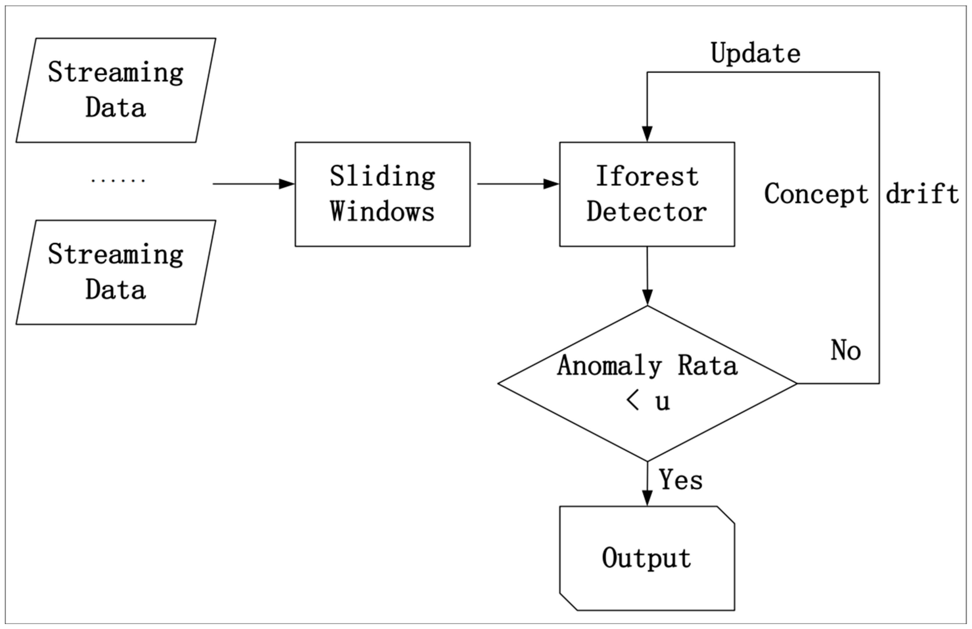
• iForestASD algorithm:
  • Time complexity: O(N∗m∗h), where N is the number of data points in the window, m is the number of trees, and h is the average height of the trees. The time complexity of the iForestASD algorithm depends on the number of data points in the window and the number of trees.
  • Space complexity: O(N∗m∗d), where d is the data dimension. The space complexity of the iForestASD algorithm is related to the size of the data in the window, the number of trees, and the feature dimension of newly arrived data points.
  • Scalability: The iForestASD algorithm has good scalability. The algorithm uses a sliding window approach to handle streaming data, allowing real-time updates of the isolation forest model and calculation of anomaly scores, thus being able to adapt to continuously incoming new data.
• LSHiforest algorithm:
  • Algorithm complexity: The time and space complexity of the LSHiforest algorithm are not mentioned in the corresponding articles. However, overall, the algorithm has low complexity and is related to the data volume and data dimension in the window.
  • Scalability: The LSHiforest algorithm has good scalability. The algorithm has low complexity and is not sensitive to parameters, making it suitable for scalable anomaly detection.

In conclusion, on the basis of the information in Table 10, the complexity and scalability of data stream anomaly detection algorithms using semi-online learning can be summarized as follows:

Regarding algorithms that combine offline training with batch updates, their overall scalability is lower compared to algorithms that combine offline training with incremental updates. This is because incremental update algorithms exhibit better adaptability to unknown anomalies.

• In the category of algorithms using offline training combined with incremental updates:
  • The algorithm based on subspace partitioning utilizes subspace data structures, providing a unique advantage in feature extraction. Consequently, it exhibits the best scalability among the other three types.
  • The algorithm based on the similarity of data distribution has complexity that correlates with the statistical characteristics of the data, resulting in relatively good scalability compared to the other three types.
• In the category of algorithms using offline training combined with batch updates:
  • The algorithm based on the similarity of data distribution has complexity that is related to the statistical characteristics of the data, leading to relatively poorer scalability compared to the other three types.
  • The algorithm based on the classification principle typically requires more computational resources and time for model training, resulting in the worst scalability among the other three types.

6.3. Online-Learning-Based Data Stream Anomaly Detection Algorithms

This section provides a detailed introduction and comparison of the time complexity, space complexity, and scalability of online-learning-based data stream anomaly detection algorithms, as shown in Table 11.

• osPCA algorithm:
  • Time complexity: O(d²∗k), where d is the dimensionality of the data stream, and k is the number of computed principal components.
  • Space complexity: O(d). The algorithm updates the principal directions by copying target instances and does not require storing the entire covariance matrix or dataset.
  • Scalability: The scalability of the osPCA algorithm is relatively poor. In large-scale data stream environments, the computational cost of updating the principal directions limits its scalability.
• OSHULL algorithm:
  • Time complexity: O(n), where n is the number of normal data points. With new normal data arrivals, the OSHULL algorithm can avoid recomputing the convex hull through online adaptivity.
  • Space complexity: O(n/m), where m is the number of nodes. The OSHULL algorithm needs to store convex hull and data point information, so its space complexity is proportional to the size of the dataset. However, the algorithm uses a distributed approach by dividing the dataset into multiple parts, which reduces the storage requirements per node through average allocation.
  • Scalability: The OSHULL algorithm has good scalability. The algorithm can adaptively adjust the convex hull, making it capable of handling different types and distributions of data. Additionally, since the dataset can be processed in a distributed manner, the algorithm can be applied to large-scale distributed systems.
• Matrix Sketch-Based Data Stream Anomaly Detection Algorithm:
  • Time complexity: The time complexity mainly depends on the size of the matrix sketch and the rate of the data stream. The update and query operations of the matrix sketch are usually constant time complexity (O(1)). Therefore, the time complexity of the algorithm is typically linear or close to linear, i.e., O(n), where n is the size or length of the data stream.
  • Space complexity: The matrix sketch is a highly space-efficient data structure that typically requires minimal memory to store the sketch’s state. Therefore, the space complexity of the algorithm is usually constant, i.e., O(1) or O(k), where k is the size of the matrix sketch.
  • Scalability: This algorithm generally has good scalability. The operations of the matrix sketch can be parallelized, allowing for easy parallelization of the algorithm to handle large-scale data streams. The size of the matrix sketch can also be adjusted as needed to accommodate different scales of data streams.
• VFDT algorithm:
  • Time complexity: O(dvc), where d is the number of attributes, v is the maximum number of values per attribute, and c is the number of classes.
  • Space complexity: O(ldv∗c), where l is the number of leaves in the tree.
  • Scalability: The VFDT algorithm has good scalability. It employs incremental learning, allowing it to handle large-scale data streams without loading the entire dataset into memory.
• CVFDT algorithm, HAT algorithm:
  • Time complexity: In CVFDT and HAT algorithms, for each new sample, the algorithm determines whether to expand the current tree by computing the Hoeffding bound. Therefore, the time complexity of the algorithm is typically approximately constant, i.e., O(1).
  • Space complexity: In CVFDT and HAT algorithms, each node only stores relevant statistical information rather than the complete dataset. Therefore, the space complexity of the algorithm is typically approximately constant, i.e., O(1). However, the HAT algorithm incorporates an adaptive sliding window that avoids storing excess window data, resulting in lower space complexity compared to the CVFDT algorithm.
  • Scalability: Both CVFDT and HAT algorithms have excellent scalability, maintaining model consistency and accuracy when processing large amounts of data.
• EFDT algorithm, GAHT algorithm:
  • Time complexity: Both algorithms have a similar time complexity of O(dvc∗h), where d is the number of attributes, v is the maximum number of values per attribute, c is the number of classes, and h is the maximum depth of the tree. However, the GAHT algorithm incorporates pruning operations, resulting in lower time complexity compared to the EFDT algorithm.
  • Space complexity: Both algorithms have a similar space complexity of O(ldv∗c), where l is the number of leaves in the tree. However, the GAHT algorithm incorporates pruning operations, resulting in lower space complexity compared to the EFDT algorithm.
  • Scalability: The EFDT algorithm and GAHT algorithm have excellent scalability. The algorithms have low complexity. Additionally, the EFDT algorithm and GAHT algorithm can be combined with other incremental learning algorithms to further improve their scalability and adaptability.
• Online Deep Learning-Based Data Stream Anomaly Detection Algorithm:
  • Algorithm complexity: Examples of online deep learning anomaly detection algorithms, such as the ADA algorithm, DAGGM algorithm, ARCUS algorithm, and S-DPS algorithm, generally have variable time and space complexity. Their complexity depends on the type of deep neural network model and the training process, which is typically high.
  • Scalability: Online deep learning-based anomaly detection algorithms have overall poor scalability. The training and updating processes of deep neural networks require significant computational resources and time, limiting the scalability of the algorithms. Handling large-scale data streams may require techniques such as distributed computing or model compression to improve scalability.

In summary, considering Table 11, the complexity and scalability of data stream anomaly detection algorithms based on online learning can be summarized as follows:

• Online deep learning algorithms generally have lower scalability compared to online shallow learning algorithms. This is because deep learning algorithms often involve the training and storage of deep neural networks, which adversely affects the scalability of online deep learning algorithms.
• Among online shallow learning algorithms: Those based on matrix sketch algorithms convert data calculations into matrix sketch calculations, providing unique advantages in terms of complexity and scalability. Thus, they have the best scalability. Those based on decision tree algorithms do not require normalization and have unique advantages in feature extraction, resulting in relatively good scalability. Those based on Similarity of Data Distribution algorithms have complexity related to statistical features of the data, requiring normalization and feature extraction steps, resulting in relatively poor scalability compared to the other three categories.

Overall, considering Table 8, Table 9, Table 10 and Table 11, the scalability of offline-learning-, semi-online-learning-, and online-learning-based data stream anomaly detection algorithms can be summarized as follows:

• Offline-learning-based data stream anomaly detection algorithms
  • Low scalability: Offline-learning-based algorithms typically require batch processing and model training over the entire dataset, which can pose computational and storage challenges for large-scale datasets or high-speed data streams.
  • Difficult to adapt to changes in real time: Since the algorithms are trained offline, they may not adapt to new patterns or changing concepts in the data stream in a timely manner, requiring retraining of the entire model.
• Semi-online-learning-based data stream anomaly detection algorithms:
  • High scalability: Semi-online-learning-based algorithms typically adapt to changes in the data stream through batch updates or incremental updates. They can partially utilize previous models or samples, reducing the computational and storage requirements and thus improving scalability.
  • Relatively real-time adaptability: The algorithms can adapt to changes in the data stream to some extent through incremental updates or partial retraining, capturing changes in new patterns or concepts.
• Online-learning-based data stream anomaly detection algorithms:
  • Highly scalable: Online learning-based algorithms generally have good scalability, enabling real-time processing of large-scale data streams and model updates.
  • Real-time adaptability: Since the algorithms learn and update the model gradually on the data stream, they can promptly adapt to changes in the data stream, providing good real-time performance.

It is important to note that the scalability of each algorithm is also influenced by other factors, such as algorithm complexity, choice of underlying models, and availability of hardware resources. Therefore, in practical applications, the performance and scalability of the algorithm need to be considered in combination, and the choice of the algorithm should be based on specific requirements.

7. Application of Data Stream Anomaly Detection Algorithms

7.1. Application Scenarios of Data Stream Anomaly Detection Algorithms

Different types of data stream anomaly detection algorithms are suitable for various business scenarios. Here are some common business scenarios and the corresponding applicable algorithms:

• Algorithm Based on Offline Learning for Data Stream Anomaly Detection
  • Significance and value: By using complete historical data for model training, it is possible to obtain relatively accurate anomaly detection models. This algorithm is suitable for scenarios that involve analyzing historical data and detecting anomalies and can be used for post-analysis, investigation, and predicting future abnormal behavior.
  • Applicable business scenarios: Business scenarios involving batch data analysis. When data streams arrive in batches and can be processed offline as a whole dataset, an algorithm based on offline learning is a suitable choice. It is applicable for analyzing historical data and detecting anomalies in scenarios such as financial fraud detection and network intrusion detection.
• Algorithm Based on Semi-Online Learning for Data Stream Anomaly Detection
  • Significance and value: Semi-online learning algorithms combine the advantages of offline and online learning, providing flexibility and adaptability. These algorithms use historical data for training during the initialization phase and adapt to new anomaly types during subsequent online learning.
  • Applicable business scenarios: Business scenarios where data stream properties change slowly. When the properties of a data stream change relatively slowly and the types of anomalies remain stable, an algorithm based on semi-online learning can be trained using historical data during the initialization phase and adapted to new anomaly types during subsequent online learning. It is suitable for scenarios where there is some expectation or prior knowledge of new anomaly types, such as network traffic analysis and equipment failure detection.
• Algorithm Based on Online Learning for Data Stream Anomaly Detection
  • Significance and value: Online learning algorithms provide real-time capabilities as they learn directly from data streams, enabling timely detection and handling of new anomalies. This algorithm can be used for real-time monitoring, fault detection, and timely warnings.
  • Applicable business scenarios: Business scenarios requiring real-time anomaly detection. When there is a need to detect and respond to anomalies in data streams in real time, and when the properties and types of anomalies in the data stream may change frequently, an algorithm based on online learning is a suitable choice. This algorithm can learn and adapt in real time to changing data and anomaly types. It is applicable in scenarios with high requirements for real-time capabilities, such as smart IoT systems and network security monitoring.

However, in real-world business scenarios, it is still necessary to select the appropriate algorithm on the basis of specific business requirements, data stream characteristics, and application needs. It is important to conduct experimental tuning and final evaluation to determine the most suitable data stream anomaly detection method.

7.2. Significance, Value, and Potential Impact of Using Data Stream Anomaly Detection Algorithms

In practical business domains, using appropriate data stream anomaly detection algorithms can help in the timely identification and response to abnormal behaviors, resulting in the following significance and value:

• Enhanced security and risk reduction: Abnormal behaviors may indicate potential security threats or risk signals. By using data stream anomaly detection algorithms, abnormal behaviors can be detected in a timely manner, thereby improving security and reducing potential risks. For example, in the field of network security, anomaly detection algorithms can be used to identify malicious attacks or abnormal traffic.
• Improved business efficiency: Abnormal behaviors can lead to business interruptions, resource waste, or decreased production efficiency. By monitoring and detecting abnormal behaviors in real time, measures can be taken promptly to address the issues, thus enhancing business efficiency. For example, in manufacturing, anomaly detection algorithms can be used to detect equipment failures or production abnormalities, allowing for timely adjustments to production plans.
• Achieving intelligent decision making and optimization: Anomaly detection algorithms can provide detailed information and insights about abnormal behaviors, supporting intelligent decision making and business optimization. By analyzing patterns and trends in abnormal behavior, underlying causes of potential issues can be identified, and appropriate measures can be taken for improvement and optimization.
• Cost and resource savings: Timely detection and handling of abnormal behaviors can reduce potential losses and costs. Anomaly detection algorithms can help identify anomalous data points, events, or behaviors, thereby reducing resource waste and minimizing the need for manual intervention.

However, using inappropriate or poorly performing anomaly detection algorithms can lead to potential impacts such as

• False positives and false negatives: Unreasonable algorithm selection or parameter settings can result in false positives (misclassifying normal behavior as anomalous) or false negatives (failing to detect true anomalies), affecting normal business operations and the accuracy of decision making.
• Data quality and accuracy: Anomaly detection algorithms require high data quality and accuracy. Issues such as noise, missing data, or incorrect labeling in input data can decrease the accuracy of anomaly detection, thus impacting the performance and results of the algorithm.
• Resource requirements and performance: Different anomaly detection algorithms have varying demands for computational resources, memory, and storage. Some algorithms may be slow in processing large-scale data streams or require high computing resources, which can limit their scalability and performance in practical applications.
• Model training and updating: In offline learning and semi-online learning algorithms, the training and updating processes of models can consume significant time and computational resources. This can pose challenges in large-scale data streams or real-time application scenarios and may result in delays or untimely anomaly detection.
• Interpretability of the algorithm: Some anomaly detection algorithms may be difficult to interpret in terms of their basis and reasoning for classifying anomalies. This can pose challenges in business decision making and problem troubleshooting. In certain industries, such as finance, there is a higher demand for the interpretability of anomaly detection results.
• Data privacy and security: Data stream anomaly detection involves monitoring and analyzing real-time data, raising concerns about user privacy and data security. Ensuring data confidentiality and security are important aspects that require special attention in practical applications.

Therefore, when applying data stream anomaly detection algorithms based on offline learning, semi-online learning, and online learning, careful consideration of specific business scenarios, data characteristics, and application requirements is necessary. Ensuring the selection of appropriate algorithms; conducting thorough experimentation and evaluation; and balancing factors such as performance, accuracy, interpretability, and resource consumption are essential to achieve optimal anomaly detection effectiveness and practical value.

8. Future Research Directions

8.1. Future Research Directions of the Authors

• According to the paper, all the involved data stream anomaly detection algorithms will be conducted by experiments. With unified data sets, each algorithm will be analyzed qualitatively and quantitatively. On the basis of the analysis, the similarities and differences of algorithms and their practical application scenarios could be reached.
• A new data stream anomaly detection algorithm is proposed on the basis of the Hoeffding tree algorithm. The algorithm has the following features: (1) green and energy efficient; (2) based on online learning; (3) anti-concept drift.

8.2. Future Research Challenges

The significant demand for big data applications has driven the rapid development of the anomaly detection field; however, there are current difficulties in the field of data stream anomaly detection research:

• Difficulties based on global information settings and partial information settings. The data under the data stream are usually massive and infinite, and it is hard to store all the data in the practical application scenario, which we called global information. Some algorithms use staged data batch processing methods for data streams, or periodically retrain anomaly detection models in order to obtain global information about the input data; as a result, anomaly detection for streaming data could be reached. However, in practical applications where data streams are becoming increasingly massive, global information about the data is becoming increasingly unavailable. Therefore, it is expected that the anomaly detection of the model and the update of the model are performed simultaneously, which is very difficult in real streaming data scenarios.
• On the basis of the difficulty of three parties balance including the speed of data stream, the speed of algorithm operation, and the accuracy. One of the characteristics of data streams is that they are fast. If anomaly detection is to be performed in real time on fast incoming data, it means that the anomaly detection algorithm must also be fast, but it always costs the accuracy of the algorithm. So, the way in which to strike the balance is also one of the difficulties of anomaly detection in data streams.
• The difficulty of the concept drift caused by data flow. Data stream anomaly detection algorithms all work in dynamic environments where data flow continuously. If the data distribution of a data stream is random, it would lead the target concept may change over time. However, most of the existing machine-learning-based work on data stream anomaly detection algorithms assume that the training samples are randomly generated according to some smooth probability distribution. The way in which to optimize the algorithm in the context of streaming data scenarios so that it has the ability to resist concept drift is necessary.

8.3. Future Research Directions

This paper proposes several possible research directions based on the challenges in the field of data stream anomaly detection:

• Real-time processing and learning capabilities. In anomaly detection algorithms for data streams, the ability to detect anomalies in real time or near real time and to update their own models in real time is crucial as data flow continuously. Therefore, on the basis of the idea of online learning and combined with different machine learning models, developing anomaly detection models with more powerful anomaly detection performance is a possible direction. Currently, the literature [62,63] has made some preliminary explorations on this issue. However, more advanced exploration and utilization balancing strategies and more advanced model update rules can be used to design more effective algorithms.
• Purification processing capabilities for data streams. In practical application scenarios of streaming data, data are generally high dimensional, redundant, and even repetitive. Therefore, combining the ideas of undersampling, oversampling, or mixed sampling [41] to preprocess data streams, selecting more valuable data for training anomaly detection models, may make anomaly detection more accurate. Currently, there is little research on this issue, and there is an urgent need to fill this gap.
• Window or incremental methods. On the basis of the idea of sliding windows and incremental processing, by modifying or combining existing batch anomaly detection algorithms, and processing and retaining only the most recent observation values when data streams arrive, storage requirements of devices can be reduced, the computational cost and storage cost of anomaly detection algorithms can be reduced, and the running time of the model can be shortened.
• Dynamic adaptive threshold selection. Generally, anomaly detection methods for data streams set a fixed threshold for anomaly detection. However, the fixed threshold may not be effective for different data distributions or different time periods. Therefore, dynamically selecting an adaptive threshold on the basis of the current data distribution or time period may be a possible direction.
• Interpretability of algorithm models. When solving real-world problems such as data anomaly detection, anomaly detection models often face challenges of mistrust, opacity, and difficulty of improvement. Moreover, in practical applications, it is often not sufficient to only detect anomalies. Especially in critical application areas, it is more desirable to discover the specific reasons for anomalies in order to further address the anomalies. Model interpretation techniques can effectively address the above issues. One important direction for future exploration is how to integrate model interpretation techniques into data stream anomaly detection algorithm models.
• The issue of improving algorithm model energy efficiency. Data stream anomaly detection algorithm models typically require real-time processing and analysis of large-scale data streams. If the algorithm models can enhance energy efficiency, it will reduce the required computational resources and energy consumption. This helps to reduce energy usage, decrease the demand for power supply, and consequently alleviate environmental pressures. Simultaneously, it holds significant importance for businesses and organizations as improving energy efficiency translates to enhancing economic benefits and competitiveness. Recently, the authors of [64] conducted preliminary explorations on the energy efficiency of algorithm models.

9. Summary and Future Directions

In the era of digital intelligence driven by information technologies such as cloud computing, big data, IoT, and blockchain, data streams continuously enter the practical applications of anomaly detection. As we often cannot obtain the global information of data, the way in which to perform real-time anomaly detection for data streams is a particularly important issue in the increasingly large and complex information age. This paper analyzed and summarized the methods for data stream anomaly detection, which can be divided into three parts: offline learning based, semi-online learning based, and online learning based, and provides theoretical support for the feasibility of each algorithm. Moreover, the paper addressed the current lack of research in the field of data stream anomaly detection under certain information environments and proposed several promising research directions for the future. Overall, there are relatively few research methods for anomaly detection in data stream scenarios, and the way to perform real-time anomaly detection in the streaming environment remains a focus of research in various fields in the future.

References

- Korycki, Ł.; Cano, A.; Krawczyk, B. Active Learning with Abstaining Classifiers for Imbalanced Drifting Data Streams. In Proceedings of the 2019 IEEE International Conference on Big Data (Big Data), Los Angeles, CA, USA, 9–13 December 2019; IEEE: New York, NY, USA, 2019; pp. 2334–2343. [Google Scholar]
- Bhatia, S.; Jain, A.; Li, P.; Kumar, R.; Hooi, B. MSTREAM: Fast Anomaly Detection in Multi-Aspect Streams. In Proceedings of the Web Conference, Ljubljana, Slovenia, 19–23 April 2021; Volume 2021, pp. 3371–3382. [Google Scholar]
- Zubaroğlu, A.; Atalay, V. Data stream clustering: A review. Artif. Intell. Rev. 2021, 54, 1201–1236. [Google Scholar] [CrossRef]
- Bahri, M.; Bifet, A.; Gama, J.; Gomes, H.M.; Maniu, S. Data stream analysis: Foundations, major tasks and tools. Wiley Interdiscip. Rev. Data Min. Knowl. Discov. 2021, 11, e1405. [Google Scholar] [CrossRef]
- Habeeb, R.A.A.; Nasaruddin, F.; Gani, A.; Hashem, I.A.T.; Ahmed, E.; Imran, M. Real-time big data processing for anomaly detection: A survey. Int. J. Inf. Manag. 2019, 45, 289–307. [Google Scholar] [CrossRef]
- Himeur, Y.; Ghanem, K.; Alsalemi, A.; Bensaali, F.; Amira, A. Artificial intelligence based anomaly detection of energy consumption in buildings: A review, current trends and new perspectives. Appl. Energy 2021, 287, 116601. [Google Scholar] [CrossRef]
- Barz, B.; Rodner, E.; Garcia, Y.G.; Denzler, J. Detecting regions of maximal divergence for spatio-temporal anomaly detection. IEEE Trans. Pattern Anal. Mach. Intell. 2018, 41, 1088–1101. [Google Scholar] [CrossRef]
- Marteau, P.F. Random partitioning forest for point-wise and collective anomaly detection—Application to network intrusion detection. IEEE Trans. Inf. Secur. 2021, 16, 2157–2172. [Google Scholar] [CrossRef]
- Din, S.U.; Shao, J.; Kumar, J.; Mawuli, C.B.; Mahmud, S.M.H. Data stream classification with novel class detection: A review, comparison and challenges. Knowl. Inf. Syst. 2021, 63, 2231–2276. [Google Scholar] [CrossRef]
- Wang, H.; Bah, M.J.; Hammad, M. Progress in outlier detection techniques: A survey. IEEE Access 2019, 7, 107964–108000. [Google Scholar] [CrossRef]
- Eltanbouly, S.; Bashendy, M.; AlNaimi, N.; Chkirbene, Z.; Erbad, A. Machine Learning Techniques for Network Anomaly Detection: A Survey. In Proceedings of the 2020 IEEE International Conference on Informatics, IoT, and Enabling Technologies (ICIoT), Dawḥah, Qatar, 2–5 February 2020; IEEE: New York, NY, USA, 2020; pp. 156–162. [Google Scholar]
- Taha, A.; Hadi, A.S. Anomaly detection methods for categorical data: A review. ACM Comput. Surv. (CSUR) 2019, 52, 1–35. [Google Scholar] [CrossRef]
- Nassif, A.B.; Talib, M.A.; Nasir, Q.; Dakalbab, F.M. Machine learning for anomaly detection: A systematic review. IEEE Access 2021, 9, 78658–78700. [Google Scholar] [CrossRef]
- Pang, G.; Shen, C.; Cao, L.; Hengel, A.V.D. Deep learning for anomaly detection: A review. ACM Comput. Surv. (CSUR) 2021, 54, 1–38. [Google Scholar] [CrossRef]
- Blázquez-García, A.; Conde, A.; Mori, U.; Lozano, J.A. A review on outlier/anomaly detection in time series data. ACM Comput. Surv. (CSUR) 2021, 54, 1–33. [Google Scholar] [CrossRef]
- Cook, A.A.; Mısırlı, G.; Fan, Z. Anomaly detection for IoT time-series data: A survey. IEEE Internet Things J. 2019, 7, 6481–6494. [Google Scholar] [CrossRef]
- Salechi, M.; Rashidi, L. A survey on anomaly detection in evolving data. ACM SIGKDD Explor. Newsl. 2018, 20, 13–23. [Google Scholar] [CrossRef]
- Souiden, I.; Omri, M.N.; Brahmi, Z. A survey of outlier detection in high dimensional data streams. Comput. Sci. Rev. 2022, 44, 100463. [Google Scholar] [CrossRef]
- Hartigan, J.A.; Wong, M.A. Algorithm AS 136: A k-means clustering algorithm. Appl. Stat. 1979, 28, 100–108. [Google Scholar] [CrossRef]
- Cover, T.; Hart, P. Nearest neighbor pattern classification. IEEE Trans. Inf. Theory 1967, 13, 21–27. [Google Scholar] [CrossRef]
- Breunig, M.M.; Kriegel, H.P.; Ng, R.T.; Sander, J. LOF: Identifying density-based local outliers. ACM SIGMOD Rec. 2000, 16, 93–104. [Google Scholar] [CrossRef]
- Tax, D.M.J.; Duin, R.P.W. Support vector data description. Mach. Learn. 2004, 54, 45–66. [Google Scholar] [CrossRef]
- Liu, F.T.; Ting, K.M.; Zhou, Z.H. Isolation Forest. In Proceedings of the 2008 Eighth IEEE International Conference on Data Mining, Pisa, Italy, 15–19 December 2008; IEEE: New York, NY, USA, 2008; pp. 413–422. [Google Scholar]
- Sathe, S.; Aggarwal, C.C. Subspace Outlier Detection in Linear Time with Randomized Hashing. In Proceedings of the 2016 IEEE 16th International Conference on Data Mining (ICDM), Barcelona, Spain, 12–16 December 2016; IEEE: New York, NY, USA, 2016; pp. 459–468. [Google Scholar]
- Munir, M.; Siddiqui, S.A.; Dengel, A.; Ahmed, S. DeepAnT: A deep learning approach for unsupervised anomaly detection in time series. IEEE Access 2018, 7, 1991–2005. [Google Scholar] [CrossRef]
- Li, L.; Yan, J.; Wang, H.; Jin, Y. Anomaly detection of time series with smoothness-inducing sequential variational auto-encoder. IEEE Trans. Neural Netw. Learn. Syst. 2020, 32, 1177–1191. [Google Scholar] [CrossRef] [PubMed]
- Akcay, S.; Atapour-Abarghouei, A.; Breckon, T.P. Ganomaly: Semi-Supervised Anomaly Detection via Adversarial Training. In Proceedings of the Computer Vision–ACCV 2018, 14th Asian Conference on Computer Vision, Perth, Australia, 2–6 December 2018; Revised Selected Papers, Part III 14. Springer International Publishing: Berlin/Heidelberg, Germany, 2019; pp. 622–637. [Google Scholar]
- Shafiq, U.; Shahzad, M.K.; Anwar, M.; Shaheen, Q.; Shiraz, M.; Gani, A. Transfer Learning Auto-Encoder Neural Networks for Anomaly Detection of DDoS Generating IoT Devices. Secur. Commun. Netw. 2022, 2022, 8221351. [Google Scholar] [CrossRef]
- Salehi, M.; Leckie, C.; Bezdek, J.C.; Vaithianathan, T.; Zhang, X. Fast memory efficient local outlier detection in data streams. IEEE Trans. Knowl. Data Eng. 2016, 28, 3246–3260. [Google Scholar] [CrossRef]
- Yoon, S.; Lee, J.G.; Lee, B.S. NETS: Extremely fast outlier detection from a data stream via set-based processing. Proc. VLDB Endow. 2019, 12, 1303–1315. [Google Scholar] [CrossRef]
- Amer, M.; Goldstein, M.; Abdennadher, S. Enhancing One-Class Support Vector Machines for Unsupervised Anomaly Detection. In Proceedings of the ACM SIGKDD Workshop on Outlier Detection and Description, Chicago, IL, USA, 11 August 2013; pp. 8–15. [Google Scholar]
- Angiulli, F.; Fassetti, F. Detecting distance-based outliers in streams of data. In Proceedings of the Sixteenth ACM Conference on Information and Knowledge Management, Lisbon, Portugal, 6–10 November 2007; pp. 811–820. [Google Scholar]
- Angiulli, F.; Fassetti, F. Distance-based outlier queries in data streams: The novel task and algorithms. Data Min. Knowl. Discov. 2010, 20, 290–324. [Google Scholar] [CrossRef]
- Kontaki, M.; Gounaris, A.; Papadopoulos, N.; Tsichlas, K.; Manolopoulos, Y. Continuous Monitoring of Distance-Based Outliers over Data Streams. In Proceedings of the IEEE 27th International Conference on Data Engineering, Hannover, Germany, 11–16 April 2011; pp. 135–146. [Google Scholar]
- Kontaki, M.; Gounaris, A.; Papadopoulos, N.; Tsichlas, K.; Manolopoulos, Y. Effificient and flflexible algorithms for monitoring distance-based outliers over data streams. Inf. Syst. 2016, 55, 37–53. [Google Scholar] [CrossRef]
- Toliopoulos, T.; Gounaris, A.; Tsichlas, K.; Papadopoulos, A.; Sampaio, S. Continuous outlier mining of streaming data in flink. Inf. Syst. 2020, 93, 101569. [Google Scholar] [CrossRef]
- Na, G.S.; Kim, D.; Yu, H. Dilof: Effective and Memory Efficient Local Outlier Detection in Data Streams. In Proceedings of the 24th ACM SIGKDD International Conference on Knowledge Discovery & Data Mining, London, UK, 19–23 August 2018; pp. 1993–2002. [Google Scholar]
- Borah, A.; Gruenwald, L.; Leal, E.; Panjei, E. A GPU Algorithm for Detecting Contextual Outliers in Multiple Concurrent Data Streams. In Proceedings of the 2021 IEEE International Conference on Big Data (Big Data), Virtual Conference, 15–18 December 2021; pp. 2737–2742. [Google Scholar]
- Ding, Z.; Fei, M. An anomaly detection approach based on isolation forest algorithm for streaming data using sliding window. IFAC Proc. Vol. 2013, 46, 12–17. [Google Scholar] [CrossRef]
- Sun, H.; He, Q.; Liao, K.; Sellis, T.; Guo, L.; Zhang, X.; Shen, J.; Chen, F. Fast Anomaly Detection in Multiple Multi-Dimensional Data Streams. In Proceedings of the 2019 IEEE International Conference on Big Data (Big Data), Los Angeles, CA, USA, 9–13 December 2019; IEEE: New York, NY, USA, 2019; pp. 1218–1223. [Google Scholar]
- Lee, Y.J.; Yeh, Y.R.; Wang YC, F. Anomaly detection via online oversampling principal component analysis. IEEE Trans. Knowl. Data Eng. 2012, 25, 1460–1470. [Google Scholar] [CrossRef]
- Novoa-Paradela, D.; Fontenla-Romero, O.; Guijarro-Berdiñas, B. Online Learning for Anomaly Detection via Subdivisible Convex Hulls. In Proceedings of the 2020 International Joint Conference on Neural Networks (IJCNN), Glasgow, UK, 19–24 July 2020; IEEE: New York, NY, USA, 2020; pp. 1–8. [Google Scholar]
- Huang, H.; Kasiviswanathan, S.P. Streaming anomaly detection using randomized matrix sketching. Proc. VLDB Endow. 2015, 9, 192–203. [Google Scholar] [CrossRef]
- Chen, H.; Chen, P.; Yu, G. A framework of virtual war room and matrix sketch-based streaming anomaly detection for microservice systems. IEEE Access 2020, 8, 43413–43426. [Google Scholar] [CrossRef]
- Hulten, G.; Spencer, L.; Domingos, P. Mining Time-Changing Data Streams. In Proceedings of the Seventh ACM SIGKDD International Conference on Knowledge Discovery and Data Mining, San Francisco, CA, USA, 26–29 August 2001; pp. 97–106. [Google Scholar]
- Bifet Figuerol, A.C.; Gavaldà Mestre, R. Adaptive Parameter-Free Learning from Evolving Data Streams; UPC Universitat Politècnica de Catalunya: Barcelona, Spain, 2009. [Google Scholar]
- Manapragada, C.; Webb, G.I.; Salehi, M. Extremely Fast Decision Tree. In Proceedings of the 24th ACM SIGKDD International Conference on Knowledge Discovery & Data Mining, London, UK, 19–23 August 2018; pp. 1953–1962. [Google Scholar]
- Garcia-Martin, E.; Bifet, A.; Lavesson, N.; König, R.; Linusson, H. Green Accelerated Hoeffding Tree. arXiv 2022, arXiv:2205.03184. [Google Scholar]
- Sahoo, D.; Pham, Q.; Lu, J.; Hoi, S.C. Online Deep Learning: Learning Deep Neural Networks on the Fly. In Proceedings of the 27th International Joint Conference on Artificial Intelligence, Stockholm, Sweden, 13–19 July 2018; AAAI Press: Washington, DC, USA, 2018; pp. 2660–2666. [Google Scholar]
- Yuan, Y.; Adhatarao, S.S.; Lin, M.; Yuan, Y.; Liu, Z.; Fu, X. Ada: Adaptive Deep Log Anomaly Detector. In Proceedings of the IEEE INFOCOM 2020—IEEE Conference on Computer Communications, Virtual, 6–9 July 2020; IEEE: New York, NY, USA; pp. 2449–2458. [Google Scholar]
- Zong, B.; Song, Q.; Min, M.R.; Cheng, W.; Lumezanu, C.; Cho, D.; Chen, H. Deep Autoencoding Gaussian Mixture Model for Unsupervised Anomaly Detection. In Proceedings of the International Conference on Learning Representations, Vancouver, VA, Canada, 30 April–3 May 2018. [Google Scholar]
- Yoon, S.; Lee, Y.; Lee, J.G.; Lee, B.S. Adaptive Model Pooling for Online Deep Anomaly Detection from a Complex Evolving Data Stream. In Proceedings of the 28th ACM SIGKDD Conference on Knowledge Discovery and Data Mining, Washington, DC, USA, 14–18 August 2022; pp. 2347–2357. [Google Scholar]
- Mahmood, H.; Mahmood, D.; Shaheen, Q.; Akhtar, R.; Changda, W. S-DPs: An SDN-based DDoS protection system for smart grids. Secur. Commun. Netw. 2021, 2021, 6629098. [Google Scholar] [CrossRef]
- Agrahari, S.; Singh, A.K. Concept drift detection in data stream mining: A literature review. J. King Saud Univ. Comput. Inf. Sci. 2022, 34, 9523–9540. [Google Scholar] [CrossRef]
- Tellis, V.M.; D’Souza, D.J. Detecting Anomalies in Data Stream Using Efficient Techniques: A Review. In Proceedings of the 2018 International Conference on Control, Power, Communication and Computing Technologies (ICCPCCT), Kannur, India, 23–24 March 2018; IEEE: New York, NY, USA, 2018; pp. 296–298. [Google Scholar]
- Hinton, G.E.; Salakhutdinov, R.R. Reducing the dimensionality of data with neural networks. Science 2006, 313, 504–507. [Google Scholar] [CrossRef]
- Zhang, X.; Dou, W.; He, Q.; Zhou, R.; Leckie, C.; Kotagiri, R.; Salcic, Z. LSHiForest: A Generic Framework for Fast Tree Isolation Based Ensemble Anomaly Analysis. In Proceedings of the 2017 IEEE 33rd International Conference on Data Engineering (ICDE), Los Angeles, CA, USA, 9–12 December 2017; pp. 983–994. [Google Scholar]
- Liberty, E. Simple and Deterministic Matrix Sketching. In Proceedings of the 19th ACM SIGKDD International Conference on Knowledge Discovery and Data Mining, Chicago, IL, USA, 11–14 August 2013; pp. 581–588. [Google Scholar]
- Halko, P.G.N.; Martinsson, J.; Tropp, A. Finding Structure with Randomness: Probabilistic Algorithms for Constructing Approximate Matrix Decompositions. SIAM Rev. 2011, 4, 53. [Google Scholar] [CrossRef]
- Sahoo, D.; Pham, Q.; Lu, J.; Hoi, S.C. Online deep learning: Learning deep neural networks on the fly. arXiv 2017, arXiv:1711.03705. [Google Scholar]
- Cho, K.; Van Merriënboer, B.; Gulcehre, C.; Bahdanau, D.; Bougares, F.; Schwenk, H.; Bengio, Y. Learning phrase representations using rnn encoder-decoder for statistical machine translation. arXiv 2014, arXiv:1406.1078. [Google Scholar]
- Alrawashdeh, K.; Purdy, C. Fast Hardware Assisted Online Learning Using Unsupervised Deep Learning Structure for Anomaly Detection. In Proceedings of the 2018 International Conference on Information and Computer Technologies (ICICT), Dekalb, IL, USA, 23–25 March 2018; IEEE: New York, NY, USA; pp. 128–134. [Google Scholar]
- Steenwinckel, B.; De Paepe, D.; Hautte, S.V.; Heyvaert, P.; Bentefrit, M.; Moens, P.; Dimou, A.; Bossche, B.V.D. FLAGS: A methodology for adaptive anomaly detection and root cause analysis on sensor data streams by fusing expert knowledge with machine learning. Future Gener. Comput. Syst. 2021, 116, 30–48. [Google Scholar] [CrossRef]
- Khan, M.K.; Shiraz, M.; Shaheen, Q.; Butt, S.A.; Akhtar, R.; Khan, M.A.; Changda, W. Hierarchical routing protocols for wireless sensor networks: Functional and performance analysis. J. Sens. 2021, 2021, 7459368. [Google Scholar] [CrossRef]