Soft Segmentation of Terrestrial Laser Scanning Point Cloud of Forests

Abstract

As the three-dimensional (3D) laser scanner is widely used for forest inventory, analyzing and processing point cloud data captured with a 3D laser scanner have become an important research topic in recent years. The extraction of single trees from point cloud data is essential for further investigation at the individual tree level, such as counting trees and trunk analysis, and many developments related to this topic have been published. However, constructing an accurate and automated method to obtain the tree crown silhouette from the point cloud data is challenging because the tree crowns often overlap between adjacent trees. A soft segmentation method that uses K-Nearest Neighbor (KNN) and contour shape constraints at the overlap region is proposed to solve this task. Experimental results show that the visual effect of the tree crown shape and the precision of point cloud segmentation have improved. It is concluded that the proposed method works well for tree crown segmentation and silhouette reconstruction from the terrestrial laser scanning point cloud data of the forest.

1. Introduction

Both natural and planted forests are essential to the pursuit of harmony between man and nature. Therefore, they are worthy of attention and research, including tree counting, shape analysis, and the extracting of structural characteristics. In recent years, laser scanning has become a convenient technology for obtaining data on forests. Although the data consist of a large number of points, named point cloud, in three-dimensional (3D) space and those points do not directly contain adjacency information, all points have accurate 3D position information, which is helpful for forest analysis.

Point cloud segmentation, for example, tree recognition and crown extraction, is the basis of forest analysis. Forest point cloud has become a hot topic in intelligent biological data processing in recent decades. Based on accurate segmentation, each tree crown is obtained and can be reconstructed into a 3D digital geometric model. This geometrical model can be used to extract and analyze geometric parameters of the tree and as the elements of virtual reality scenes (3D animation and movie, etc.).

Regarding forest point cloud segmentation, existing representative methods related to our main contributions can be classified into two categories: individual tree identification and tree crown shape extraction.

Individual tree identification is an important research topic for supporting the collection of automatic field inventory using Light Detection and Ranging (LiDAR) technology [1]. Common methods or ideas include layer stacking, mean shift or region growth, bottom-up or up-down, clustering, and characteristic analysis based on differential quantity.

The layer stacking method for forest point cloud segmentation is used to slice the forest point cloud at fixed (0.5 m, for example) height intervals and detect trees in each layer, merging the results from all layers to build all tree profiles [2]. Similar to layer stacking, Hamraz H et al. [3] proposed a tree segmentation method for multi-story stands that stratifies the point cloud to canopy layers and segments individual tree crowns within each layer using a digital surface model-based tree segmentation method.

Some of the literature adopted mean shift or region growth methods to segment forest point clouds. Wen X et al. [4] completed an experimental assessment of the mean shift algorithm for the segmentation of airborne LiDAR data. Ma Z et al. [5] presented a two-stage method to detect individual trees from LiDAR data and adopted a region-growing algorithm to complete the initial segmentation. Liu Q et al. [6] presented a trunk-growth method with normal vector directions for single tree point cloud segmentation and applied this method to the primeval forest scenes. Wang D et al. [7] proposed an automatic data-driven approach to extract individual trees from a large-area terrestrial point cloud based on the point cloud graph by pathfinding.

The bottom-up or up-down methods are explored for forest point cloud segmentation. Lu X et al. [8] built a bottom-up algorithm using point cloud data’s intensity and 3D structure to segment deciduous forests.

In addition, hybrid clustering techniques are also used for forest segmentation. Chen Q et al. [9] proposed a hybrid clustering technique by combining DBSCAN (Density-Based Spatial Clustering of Applications with Noise) and K-means for segmenting individual trees from airborne LiDAR point cloud data. For terrestrial backpack LiDAR data, Cebral L et al. [10] used an individual tree extraction method based on DBSCAN clustering and cylinder voxelization of the volume. To avoid under- and over-segmentation effects, Dersch et al. [1] presented an integrated single tree segmentation using a graph-cut clustering method that is supported by automatic stem detection. Sebastian D et al. [11] proposed a method for individual tree stem detection using a graph-cut clustering method.

A forest point cloud can also be segmented by employing characteristic analysis based on differential quantity, including normal vector and principal curvature. For example, given that the directions of the normal vector of the trunk points are in general consistent, trunks in a terrestrial scanning forest point cloud can be detected and then the individual trees can be isolated [12].

The second category of forest point cloud segmentation mainly emphasizes tree crown segmentation or tree extraction through tree crown segmentation.

Some methods emphasize using a priori knowledge, density analysis, clustering, and region growing. To obtain the accurate tree crown model with a complex structure from airborne LiDAR data for latter feature extraction, the method of Tang et al. [13] consists of several phases: filtering, transformation to a grayscale image, contrast enhancement, the opening and closing operation, and the watershed segmentation. Wang P et al. [14] completed the initial canopy segmentation using a normalized cut segmentation with a priori knowledge about the position of each tree. Given that closely located and intersected trees are often clustered together as multi-tree components, Xiao W et al. [15] suggested a tree-shaped model-based continuously adaptive mean shift algorithm. Minaík et al. [16] presented an algorithm for individual tree crown delineation that uses the excess green index, the marker-controlled watershed segmentation, the region growing algorithms, and a buffer around a treetop. Sun H et al. [17] adopted a point cloud density model, a local maximum algorithm with optimal window size, to improve the watershed algorithm for extracting the tree crowns. Shahzad M et al. [18] adopted the unsupervised mean shift clustering to segment a forest point cloud and then used the 3D ellipsoid model to fit the points of each cluster. By this way, the geometrical tree parameter’s location, height, and crown radius are extracted. Dong Z [19] built a multi-layered tree extraction method using a graph-based segmentation algorithm for segmenting the canopy and the sliding window detection method for other parts of understory trees.

Other literature put more attention to the geometry shape or topology information of the tree crown. Novotn J [20] proposed an approach to the tree crown segmentation process that combines the seeded region growing with an active contour to approximate a crown boundary. For correcting deviations caused by topography based on individual tree crown segmentation, Duan Z et al. [21] took into account the weight with normalized canopy height and the precise Digital Elevation Model (DEM) derived from the point cloud that is classified by a multi-scale curvature classification algorithm. For airborne LiDAR data, Strimbu V et al. [22] proposed a segmentation method that captures the forest’s topological structure in hierarchical data structures, quantifies topological relationships of tree crown components in a weighted graph, and finally partitions the graph to separate individual tree crowns. This bottom-up segmentation strategy is based on several quantifiable cohesion criteria that measure belief on two crown components.

In addition, a study found that combining airborne laser scanning with multiple and hyperspectral data could improve the accuracy of tree crown segmentation [23].

These representative methods are very diverse in tree crown reconstruction, a critical step of tree reconstruction [24]. Pyysalo U [25] used the obtained vector model to extract features and reconstruct single tree crowns from laser scanner data. Chao Z et al. [26] proposed an approach for tree crown reconstruction based on improving alpha-shape modeling, where the data are points unevenly distributed in a volume rather than on a surface only. Hyyppa [27] presented an attempt at combining the mobile mapping mode and a multi-echo-recording laser scanner, as well as a new methodology based on the resulting single-scan point clouds, for enhancing the integrity of individual tree crown reconstruction. To address the challenge from leaf/branch occlusions, mirroring the half-crowns facing the Mobile Laser Scanning (MLS) system to the other sides can be assumed as a solution strategy. Kato A et al. [28] employed an implicit surface to reconstruct the exact shape of an irregular tree crown of various tree species based on the LiDAR point cloud and visualize their actual crown formation in three-dimensional space.

The existing published literature indicates that the accuracy of tree counting and DBH (diameter at breast height) measuring from forest point cloud data is relatively high, which can meet the practical needs of the current forest inventory. However, the research progress of tree crown reconstruction is relatively small in recent years. Most of the existing tree crown segmentation methods are hard segmentation, and the division between overlapping trees is directly cut by a vertical plane, resulting in a plane shape of the segmentation area, which does not like the natural shape of the tree crown. In addition, the accuracy of crown point cloud segmentation affects the reconstruction effect of the tree crown shape. Therefore, for obtaining the realistic canopy silhouette shape, a soft segmentation algorithm of the forest point cloud is proposed in this study. The technical details are described in the next section.

2. Data and Methods

Synthetic forest data are used for illustrating the proposed method and evaluating its effectiveness and efficiency. Real laser scan data are used to show the results of the analysis with the proposed method.

2.1. Data

2.1.1. Synthetic Forest Data

The point cloud of the 4 pine trees, named Pine A, Pine B, Pine C, and Pine D, as shown in Figure 1, used in our experiment are captured using a Cyrax or RIGEL scanner in the Peking University campus, Beijing. Because each tree is far from its surrounding trees at the scanning site, we can easily extract each tree using 3D interactive software with the scanner. The number of points in each scan and the length of every edge along the Axially Aligned Bounding Box (AABB) of each tree are listed in

Table 1. Information of the 4 pines’ laser scan data.

Pine Na	Point N	Scene L	Scene W	Scene H
Pine A	311,505	12.648	13.841	13.686
Pine B	487,555	10.182	9.306	11.932
Pine C	116,940	10.308	12.254	8.241
Pine D	269,366	8.469	11.188	11.113

Note: the unit of length used in this paper is meter (m).

. In this table, “Pine Na” is the name of the pine, and “Pine N” is the number of points of the pine; “Scene L”, “Scene W”, and “Scene H” are the length (unit: meter) along the x-axis, y-axis, and z-axis of the AABB, which indicate the size of a tree or a forest scene. Each point is represented by 3D coordinates (x, y, z).

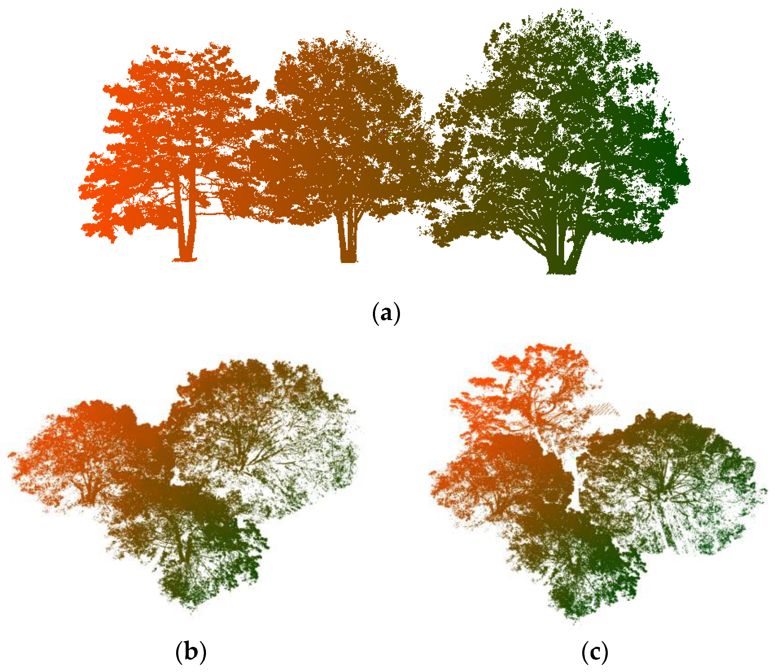
For testing the proposed soft segmentation algorithm of forest laser scanning data, several forest scenes are built by combining several tree point clouds according to the different positional relationships, including linear (Forest A, Figure 2a), triangular (Forest B, Figure 2b) and quadrangular (Forest C, Figure 2c). Using these data, the accuracy of crown segmentation can be evaluated well. The information on these built small forest point clouds is listed in

Table 2. Information on three small forests.

Forest Na	Tree N	Point N	Scene L	Scene W	Scene H
Forest A	3	1,068,426	13.017	29.802	13.686
Forest B	3	1,068,426	21.072	17.680	13.686
Forest C	4	1,185,366	21.087	23.774	13.686
Forest D	8	2,370,732	21.587	44.774	13.686

.

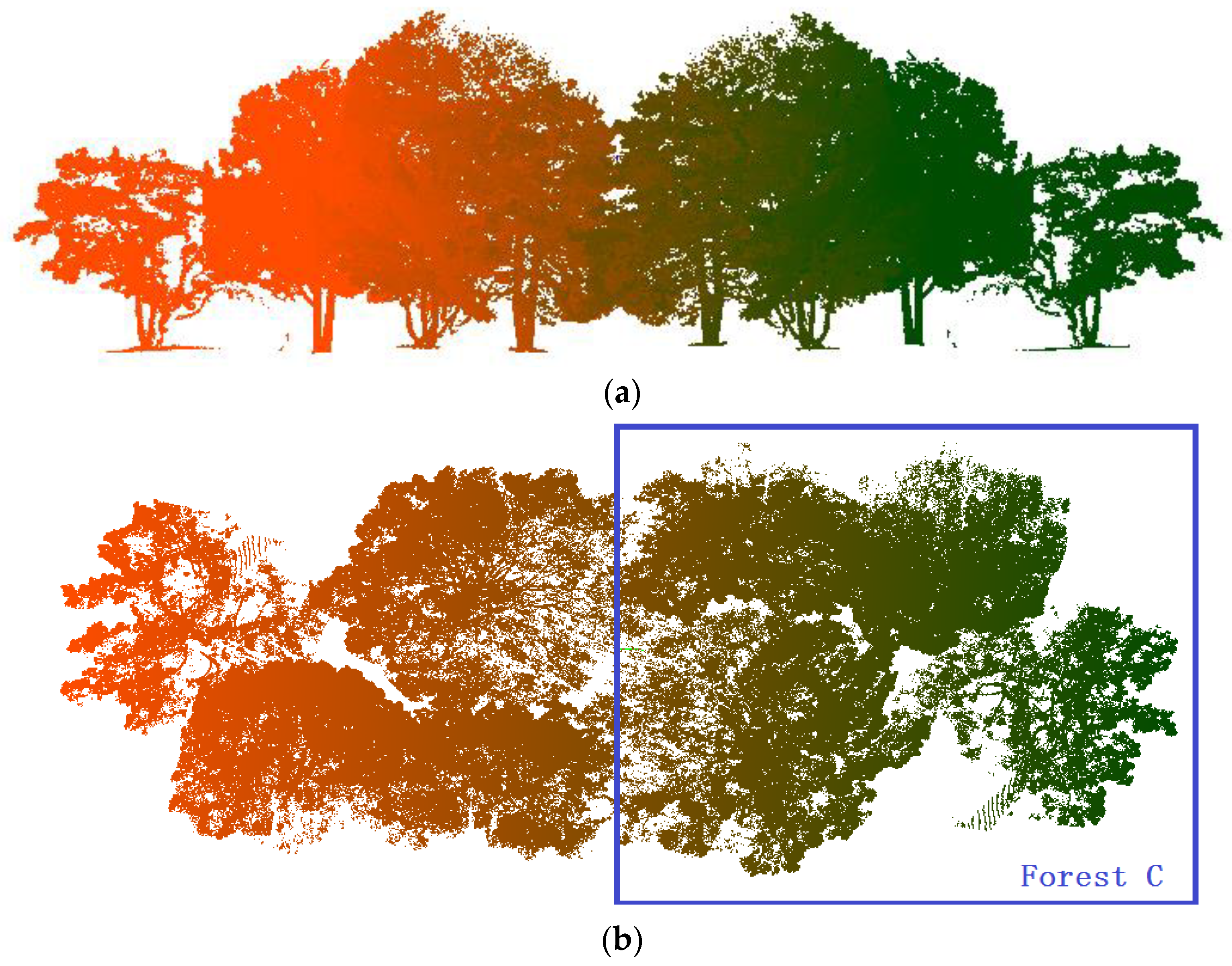
In addition, a small forest, Forest D, built using 8 trees, consists of Forest C and the transformation results of Forest C. The transformation comprises a translation vector $\left(-0.5, 21, 0\right)$ and a rotation transformation (rotation of 180 degrees around the z-direction). The pictures of Forest D from different views are shown in Figure 3. The information of the forest point cloud is also listed in Table 2.

2.1.2. Real Forest Point Cloud

A real forest point cloud, RUSH06, is used to evaluate the proposed method. RUSH06, as shown in Figure 4, was a plot, and the laser scan data was acquired in the native Eucalypt Open Forest (dry sclerophyll box-ironbark forest) in Victoria, Australia [29]. The information on the forest point cloud is also listed in

Table 3. Information of the forest scan data, RUSH06.

Forest Na	Tree N	Point N	Scene L	Scene L	Scene L
RUSH06	34	14,500,905	82.259	76.570	25.164

.

2.2. Soft Segmentation Algorithm

Our forest point cloud segmentation algorithm, soft segmentation algorithm, consists of several steps: preprocessing, partitioning with region growth algorithm, modified hard segmentation, and refining by K-Nearest Neighbor (KNN) search and contour constraints.

2.2.1. Preprocessing

Forest point cloud data generally contains a large number of points, resulting in low computational efficiency and high time costs. Therefore, at the preprocessing stage, points that are not within the scope of the study should be removed [30]. Another process is down-sampling, which was often used to accelerate point cloud registration [31].

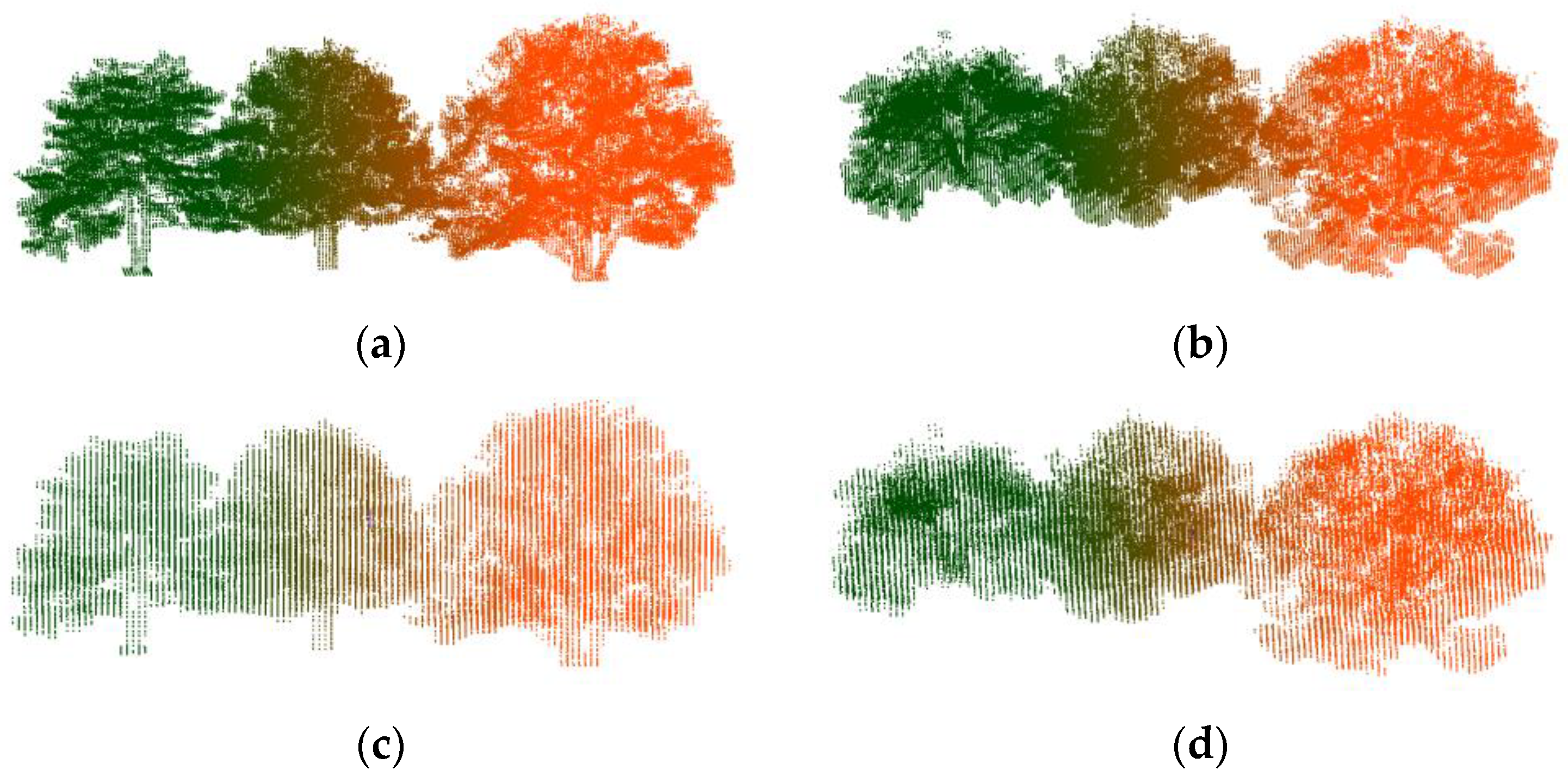
We used a down-sampling method [32] to simplify the raw point cloud. For example, after down-sampling, the number of points of Forest A (Figure 2a) can be decreased from 1,068,426 to 90,044 (8.428%) and 38,619 (3.615%) with different sampling intervals, 0.15 and 0.25, respectively, as shown in Figure 5. Although the shape of the stems has become blurred, the silhouette of the crown is kept well, and the density of the simplified point cloud is more unified. By comparing the visual effect and the compression ratio of the number of points, the default value of the sampling interval is set to 0.15 as a constant in our algorithm.

In addition, before tree identification, the ground points are removed according to the consistency of directions of normal vectors of points [12].

2.2.2. Partitioning with Region Growth Algorithm

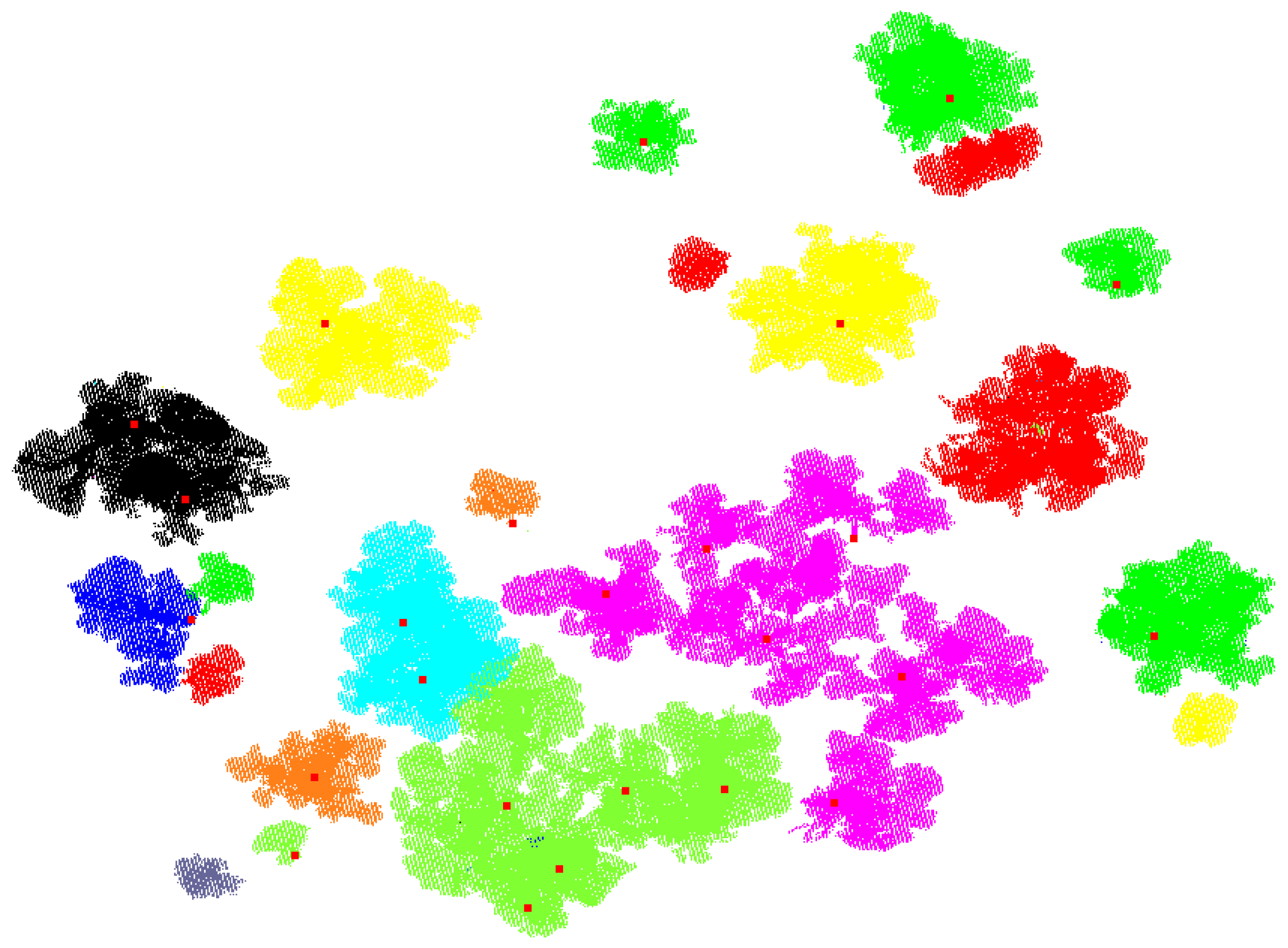
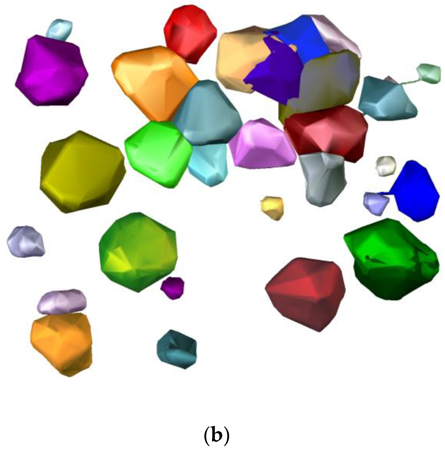
The tree identification can be practiced with the region growth algorithm for a forest where the distance between the nearest trees is considerable and tree crowns are not overlapping. If only some tree crowns are without overlap, the region growth algorithm can be used to partition the whole point cloud scene into several groups that consist of a part of tree point clouds. For example, point cloud RUSH06 (Figure 4) can be divided into 21 groups, as shown in Figure 6.

In Figure 6, the red points in each group are tree roots estimated with the clustering method and are defined using the lower several-layer points [12].

2.2.3. Modified Hard Segmentation

At first, the traditional hard segmentation algorithm is described in the following.

After the rough segmentation, the next step is to detect the individual tree from the group points that have overlap regions with the neighboring tree crowns. Similar to the literature [33], the Delaunay graph is built with roots as sites, which can be used to search the neighboring trees.

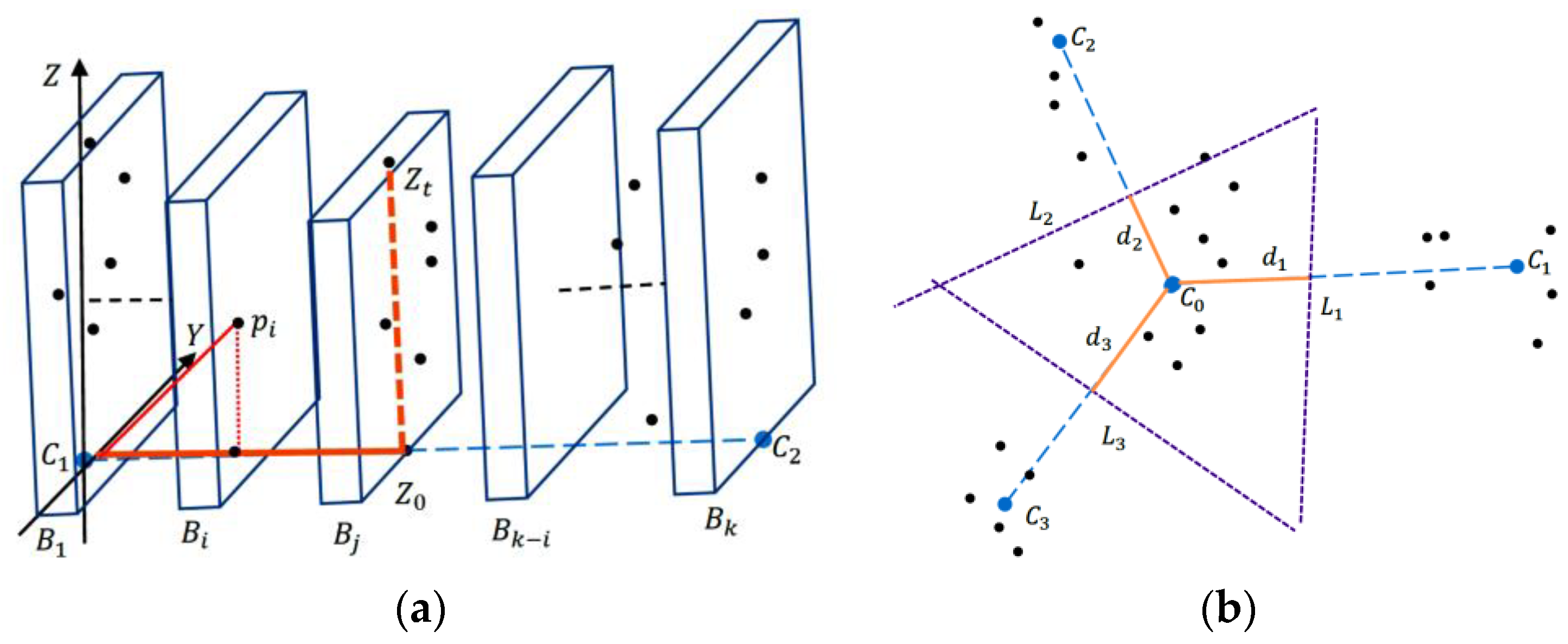
According to the Delaunay graph, we use the minimum cut plane to partition two neighbor trees. The first step is to partition points into vertical slices. Assuming that the thickness ${\Delta }_{vb}$ of each slice is 0.2 m, then the number of slices $N_{vb}$ is the quotient obtained by dividing the distance between $C_1$ and $C_2$ by ${\Delta }_{vb}$, i.e.,

$$N_{vb}=\frac{\left|C_1{C}_2\right|}{{\Delta }_{vb}},$$

(1)

where $C_1$ and $C_2$ are the roots of two adjacent trees.

Figure 7a illustrates the method of generating slices along line $C_1$ to $C_2$. Note that the partition is performed in a 3D space, and the local coordinate system $\left[C_1; {\overrightarrow{C_1{C}_2}}^o,\overrightarrow{C_{1}Y}, \overrightarrow{C_{1}Z}\right]$ has been built. In this coordinate system, ${\overrightarrow{C_1{C}_2}}^o,\overrightarrow{C_{1}Y}$, and $\overrightarrow{C_{1}Z}$ are all unit vectors, and ${\overrightarrow{C_1{C}_2}}^o//\overrightarrow{C_1{C}_2}$, $\overrightarrow{C_{1}Z}=\left(0,0,1\right)$ and $\overrightarrow{C_{1}Y}=\overrightarrow{C_{1}Z}\times {\overrightarrow{C_1{C}_2}}^o$. Let $C_1\left(x_c,y_c,z_c\right)$, then any point $p_i\left(x_i,y_i,z_i\right)$ belongs to the $i^{th}$ slice $B_i$, if $i=\left|\frac{\sqrt{{\left(x_i-x_c\right)}^2+{\left(y_i-y_c\right)}^2}}{{\Delta }_{vb}}\right|$. By this way, all points in ${\mathsf{\Omega }}_C^{\left(s\right)}$, which is the point set after the down-sampling of input data, are partitioned into m slices.

The second step is to find the optimal dividing line, which is defined by the minimum cut plane and can be obtained with the solution of the minimum–maximum optimal problem as follows:

$$i^{*}=\arg \underset{i}{\min }\underset{j}{\max }\{z_j|\forall p_j\left(z_j,z_j,z_j\right)\in B_i\}$$

(2)

For convenient application, the optimal segment place series number $i^{*}$ is transformed to the distance $d^{*}$, as follows:

$$d^{*}=\langle {\Delta }_{vb}·i^{*}\rangle$$

(3)

In Equation (3), symbol $\langle x·y\rangle$ is the inner product of vectors $x$ and $y$.

In this way, the problem of judging which side of a plane any point lies on is transformed into judging based on the projection distance along the direction ${\overrightarrow{C_1{C}_2}}^o$, i.e., when

$$\langle \overrightarrow{C_1{p}_l}·{\overrightarrow{C_1{C}_2}}^o\rangle <d^{*}$$

(4)

Point $p_i$ is at the same side as $C_1$ of the cut plane, denoted as $p_i\in \partial \left(C_1, C_2\right)$.

The last step is to find all points that belong to the individual tree. The label $L\left(p_i\right)$ of a point $p_i\left(x_i,y_i,z_i\right)$ is determined by a partitioning rule:

$$L\left(p_i\right)=L\left(C_0\right), if p_i\in {{\displaystyle \cap }}_i\partial \left(C_0, C_i\right),$$

(5)

where $C_i$ is the neighbor root of $C_0$ according to the Delaunay graph, as shown in Figure 7b. In fact, Equation (5) means that if point $p_i$ and root $C_0$ are always on the same side of the minimum cut planes that are between root $C_0$ and roots $C_i$, the label of point $p_i$ is set as the label of root $C_0$, i.e., point $p_i$ and root $C_0$ are inferred to come from the same tree.

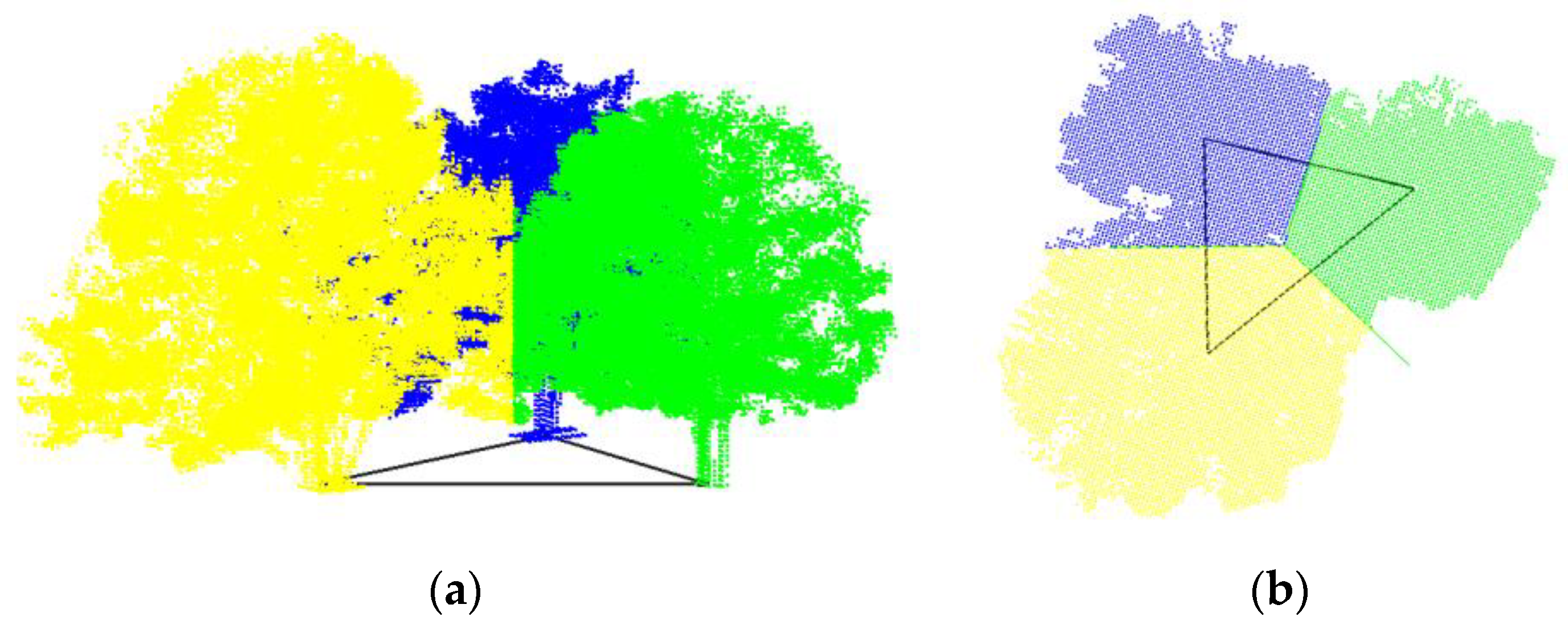
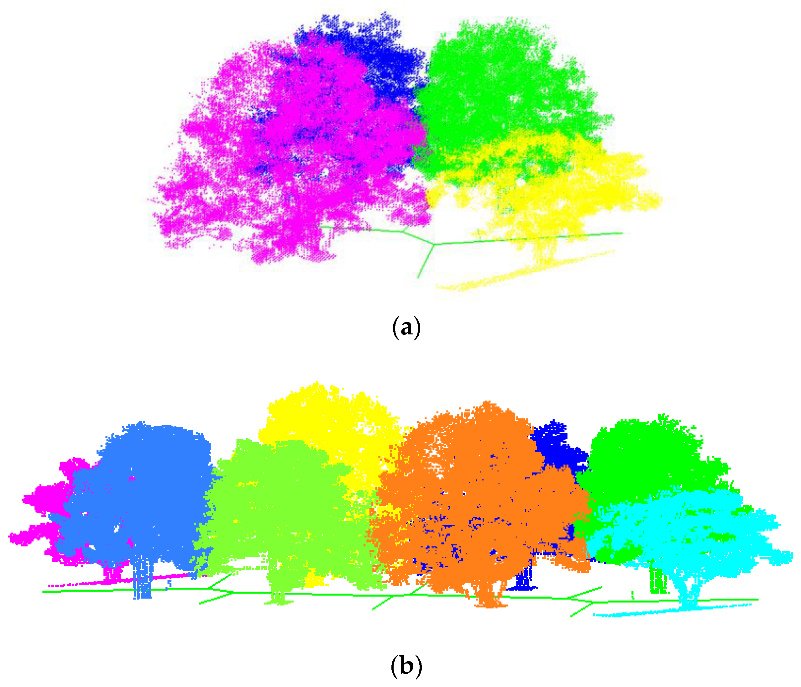
Equation (5) defines a hard vertical partitioning (tagged as hard segmentation), which segments the point cloud (Figure 2b) into Figure 8 after down-sampling. From the figure, it can be found that after segmenting, the shape between the two segmented crowns is a straight line. This is generally not a natural shape, which cannot display the overlap between the adjacent tree crowns.

To improve the visual effect of the crown shape generated with the hard segmentation algorithm, a modified hard segmentation algorithm is proposed. This algorithm adopts the idea that those points near the intersection region are treated as unlabeled points set after hard segmentation.

In this modified hard segmentation algorithm, different from Equation (5), some patches near the best bin (Equation (2)) are set as pending regions. The width of each pending region is a positive parameter and is specified with experiments. In our experiments, the width of each pending region is 0.47 m. The segmentation effect of Forest B using this approach can be illustrated in Figure 9.

2.2.4. Refined by KNN and Contour Constraints

To determine which tree these points at the pending region belong to, three steps are proposed as follows.

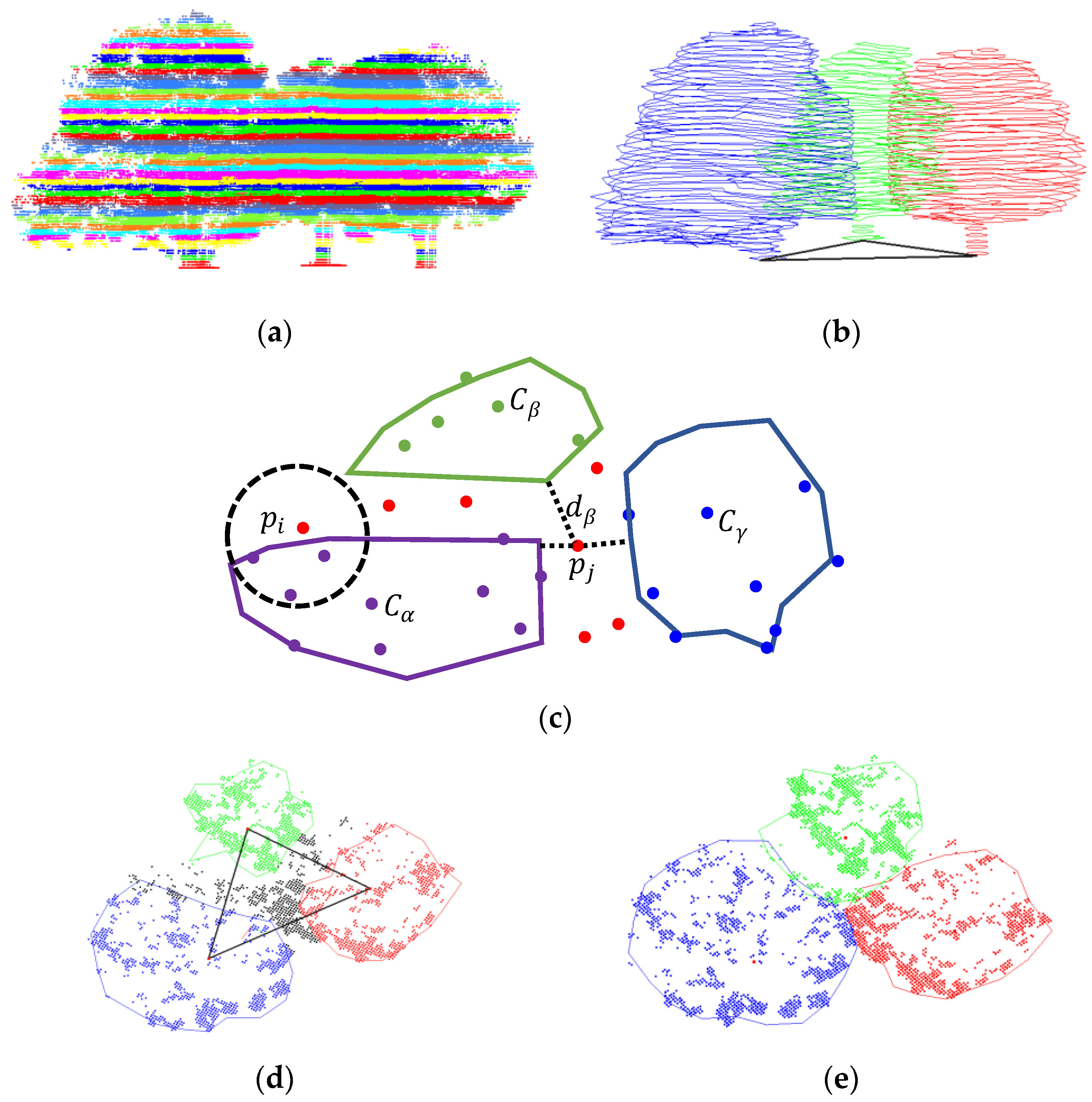
Step 1: Generating horizontal layers. Given that the overlap of adjacent crowns only occurs at some layers, the forest point cloud can be segmented in a horizontal direction. The thickness of each layer is a constant number, for example, 0.4 m. The experimental result is shown in Figure 10a.

Step 2: Build the contours of all layers. Based on the results of modified hard segmentation and the generation of horizontal layers, the contour curve of each layer in every initial individual tree point cloud can be constructed using the 2D alpha-shape method [34], as shown in Figure 10b. This initial contour, used as the boundary of partitioning individual trees, has more options than the constraints resulting only from the contour generated by projecting points onto the ground.

Step 3: Refining by KNN and contour constraints. For these unlabeled regions, an approximate K-Nearest Neighbor (KNN) algorithm [35] is employed to label some unclassified points. For an unclassified point $p_i$ in the pending region, as the dashed black circle shown in Figure 10c, the classifying rule is as follows:

$$L\left(p_i\right)=\{\begin{array}{c}L\left(C_{\alpha }\right), \mathrm{if} r_{nei}>0.8\\ pending, otherwise \end{array} ,$$

(6)

where

$$r_{nei}=\frac{n_{nei}}{K}$$

(7)

In Equation (7), $K$ is the number of neighbor points of $p_i$, and $n_{nei}$ is the number of neighbors that are the same label as the classified point $C_{\alpha }$. After this step, there are still some unclassified points.

Then, we used a Monte Carlo method to label those unclassified points according to the probability.

$$P_{label}=e^{-d_i/\sigma }.$$

(8)

In Equation (8), $d_i$ is the distance from point $p_i$ to the contour of this layer; $\sigma$ is a positive number and set by experiment. The idea behind this equation is that the farther away from the contour of one tree, the small the probability of belonging to this tree.

After using the refine segmentation algorithm, the contours of these segmented individual trees (Figure 10e) look more natural than the results using the hard segmentation algorithm (Figure 10d).

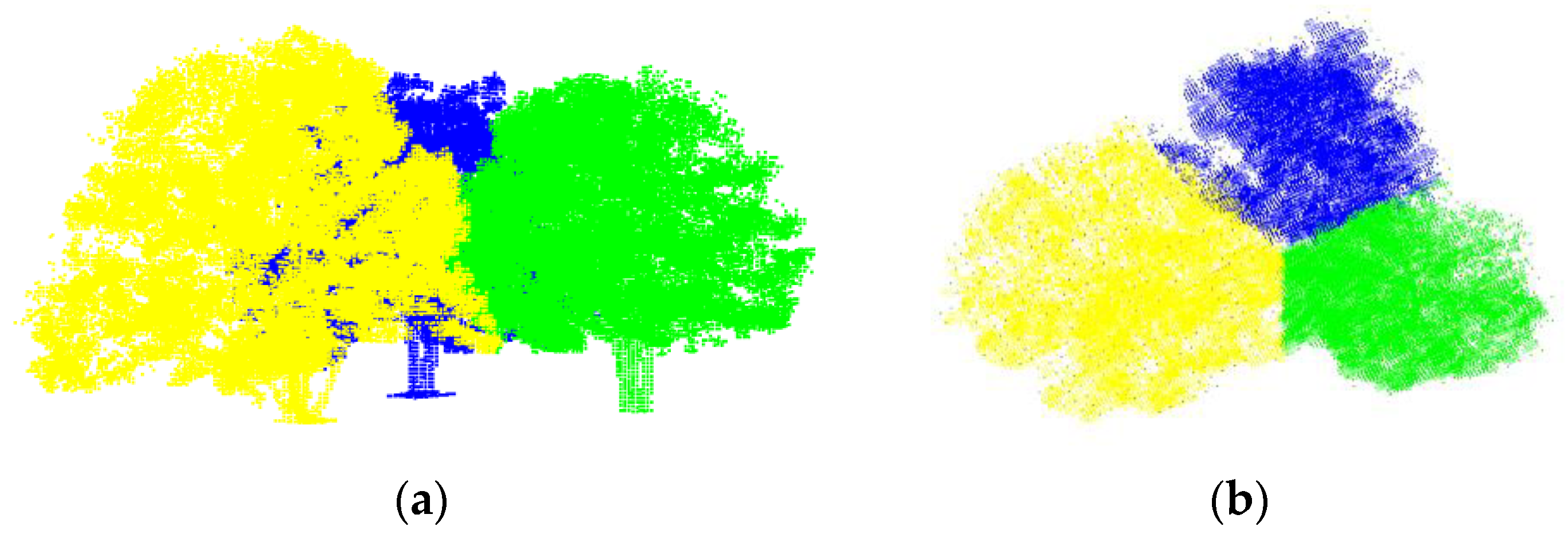
At last, the segmented individual trees using our method are displayed in Figure 11. From the figure, it can be seen that the division of overlapping areas of tree crowns appears more natural than in Figure 8.

2.3. Tree Crown Silhouette Extracted and Reconstruction

To conveniently obtain the geometric shape attributes and digital mesh model of the tree crown, the segmented individual tree point clouds are taken as the input for crown surface reconstruction. By re-sampling the contours of all layers, the surface points with uniform distribution on the crown silhouette can be obtained. Then, the crown surface geometry can be reconstructed based on a 3D $\mathsf{\alpha }$-shape [34] or modified $\mathsf{\alpha }$-shape method [36].

With the reconstructed tree mesh models, some attributes of the tree crown, including width, height, superficial area, and projecting ground area can be easily estimated.

The width $W_{crown}$ of a tree crown is estimated according to Equation (9):

$$W_{crown}=\max \left\{\left|\overline{P_i^{\prime }{P}_j^{\prime }}, \forall P_i^{\prime },P_j^{\prime }\in \mathsf{\Gamma }\right|\right\},$$

(9)

where $\mathsf{\Gamma }$ is the boundary of projection points set that vertical mapping $\mathsf{\Lambda }$ onto the xOy plane.

The height $H_{crown}$ of the crown can be estimated with laser scanning point data:

$$H_{crown}={ \mathrm{Z}}_{\max }-{ \mathrm{Z}}_{\min },$$

(10)

where ${\mathrm{Z}}_{\max }$ and ${\mathrm{Z}}_{\min }$ are the maximum and minimum z-coordinates of the crown.

The superficial area of the crown is the sum of the areas of all triangles on the surface of the crown. In the traditional $\mathsf{\alpha }$-shape method, the triangles in the crown perhaps are turned into boundary triangles if the radius r of the probing ball is too small. This led to a bigger superficial area than the real case. In addition, if the r is set too large, the reconstructed crown will become a convex hull, which also induces a significant error. As our method only uses boundary points to build the crown surface, the superficial area only consists of boundary triangles, making the error small.

For calculating the projecting ground area, all points of $\mathsf{\Lambda }$ are projected onto the xOy plane, and a polygon $𝒫$ is built on these projected points by employing the 2D $\mathsf{\alpha }$-shape method. Note that the polygon $𝒫$ may not always be convex, and the built $𝒫$ based on projecting C or $\mathsf{\Lambda }$ onto the xOy plane is the same.

3. Results

We demonstrate the effectiveness of the proposed algorithm based on point cloud segmentation and reconstruction experiments. Our algorithm was written in C++ Language with the support of OpenGL for visualization. Experiments were made on a laptop with Intel(R) Core(TM) i7-4710MQ [email protected] and RAM 4.0G.

For quantitatively evaluating the effect of segmentation of our method, we compare our results to that from the hard segmentation (Section 2.2.3) using three evaluation metrics, including accuracy (Acc), mean class accuracy (mAcc) [37], and mean Intersection over Union (mIoU).

The accuracy (Acc) is calculated using the following formula:

$$\mathrm{Acc}=\frac{1}{N}{\sum }_{i=1}^k{m}_{ii}.$$

(11)

The sensitivity is calculated as follows:

$$\mathrm{mAcc}=\frac{1}{k}{\sum }_{i=1}^k\frac{m_{ii}}{N_i},$$

(12)

where $m_{ij}$ is the number of points from Tree $i$ classified to Tree $j$ and $N$ is the total number of points in input data.

The index, mean Intersection over Union (mIoU), is calculated by Equation (13) as follows:

$$\mathrm{mIoU}=\frac{1}{k}{\sum }_{i=1}^k\frac{m_{ii}}{{\sum }_j\left(m_{ij}+m_{ji}\right)-m_{ii}}$$

(13)

3.1. Synthetic Forest

In view of three quantitatively evaluating indexes, we compare the results generated with our method (soft segmentation) to that of the hard segmentation method (Section 2.2.3). The values of three indexes, Acc, mAcc, and mIoU, are listed in

Table 4. The quantitative evaluation of segmentation results of four forest point clouds using three indexes.

Method	Hard Segmentation			Soft Segmentation
	Acc	mAcc	mIoU	Acc	mAcc	mIoU
Forest A	0.9801	0.9815	0.9622	0.9827	0.9845	0.9672
Forest B	0.9563	0.9624	0.9172	0.9639	0.9691	0.9318
Forest C	0.9595	0.9679	0.9319	0.9672	0.9749	0.9456
Forest D	0.9463	0.9556	0.9066	0.9575	0.9652	0.9262
Average (%)	0.9606	0.9669	0.9295	0.9678	0.9734	0.9427

. From the table, it can be found that the soft segmentation has better performance than the hard segmentation method in all three indexes and in all four small forest point clouds. On average, with our method, the rates of Acc, mAcc, and mIoU have increased by 0.76%, 0.68%, and 1.42% over that with the hard segmentation method. This ratio is relatively small because the number of points in the entire point cloud is rather large, and the number of points in the overlap region is relatively small. Therefore, a slight increase in the ratio significantly impacts the evaluation of the effect of segmenting the overlap region.

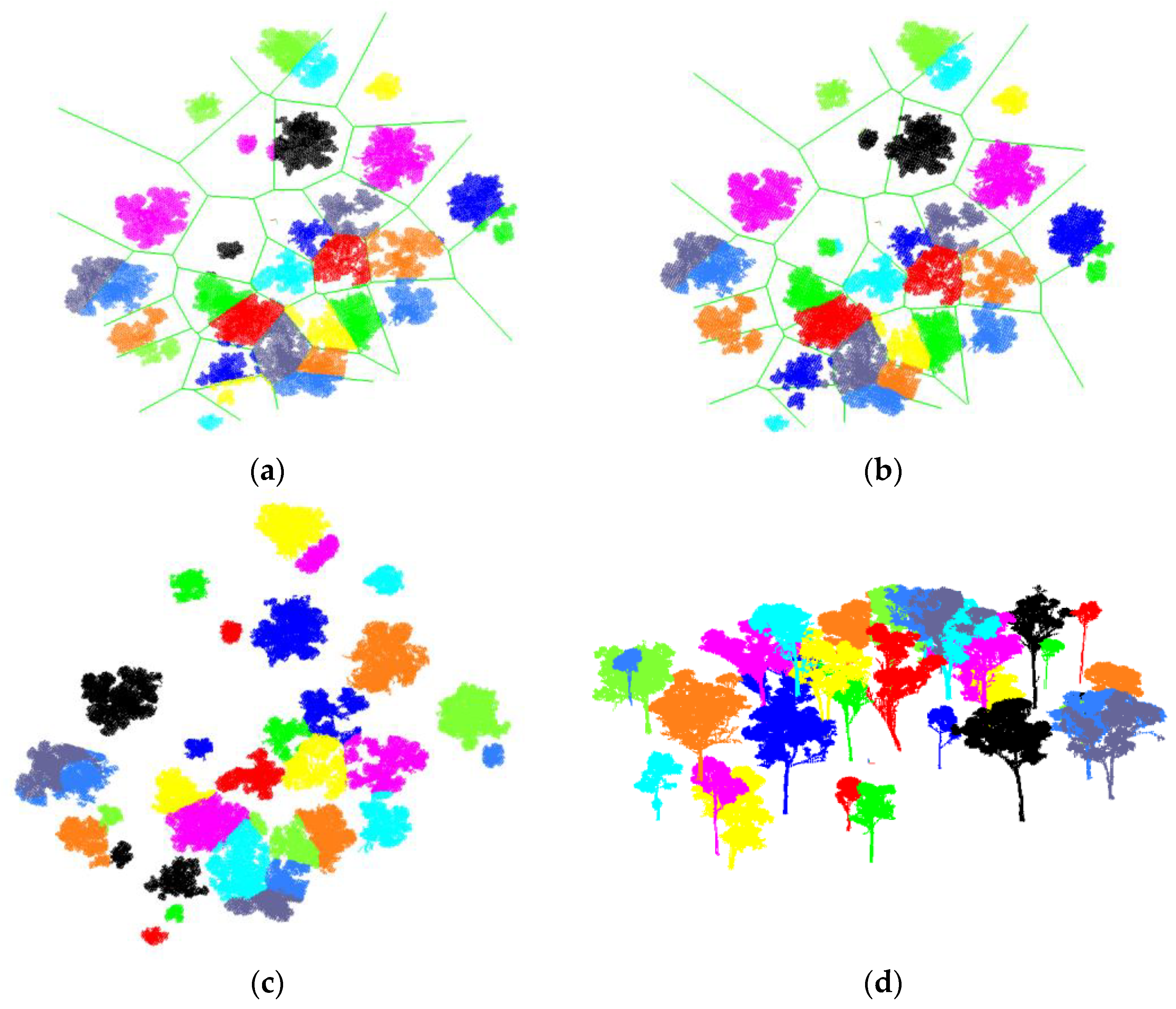
The segmented results of Forest B can be shown in Figure 10; other experimental results are displayed as follows: Figure 12 shows the segmentation result using the proposed soft segmentation method. Finally, the segmentation results of Forests C and D are illustrated in Figure 13.

3.2. Real Scanning Data

We calculate the quantitatively evaluating indexes, Acc, mAcc, and mIoU, according to the results segmented by hard segmentation algorithm (Hard Seg.), soft segmentation without region growing as preprocessing (Soft Seg. without RG), and soft segmentation with region growing as preprocessing (Soft Seg. with RG). The values of the three indexes are listed in

Table 5. The quantitative evaluation of segmentation results of RUSH06.

Method	Acc	mAcc	mIoU
Hard Seg.	0.859	0.8791	0.7279
Soft Seg. without RG	0.8587	0.8205	0.6826
Soft Seg. with RG	0.9516	0.9632	0.9272

. From the table, it can also be found that the soft segmentation with region growing as preprocessing gets the best performance among the three methods. With our method, the rates of Acc, mAcc, and mIoU have increased by at least 10.8%, 9.6%, and 27.4%.

Different from those dense forests, the distribution of trees in forest RUSH06 is uneven, with some trees farther away from others. Therefore, the segmentation effect (Figure 14c) has been greatly improved compared to the hard segmentation method (Figure 14a) and to the method of soft segmentation without the region growth step (Figure 14b). The proposed method is used to deal with those small groups that have overlap regions between adjacent trees in each group. At last, the segmentation results are shown in Figure 14c,d.

3.3. Forest Reconstruction

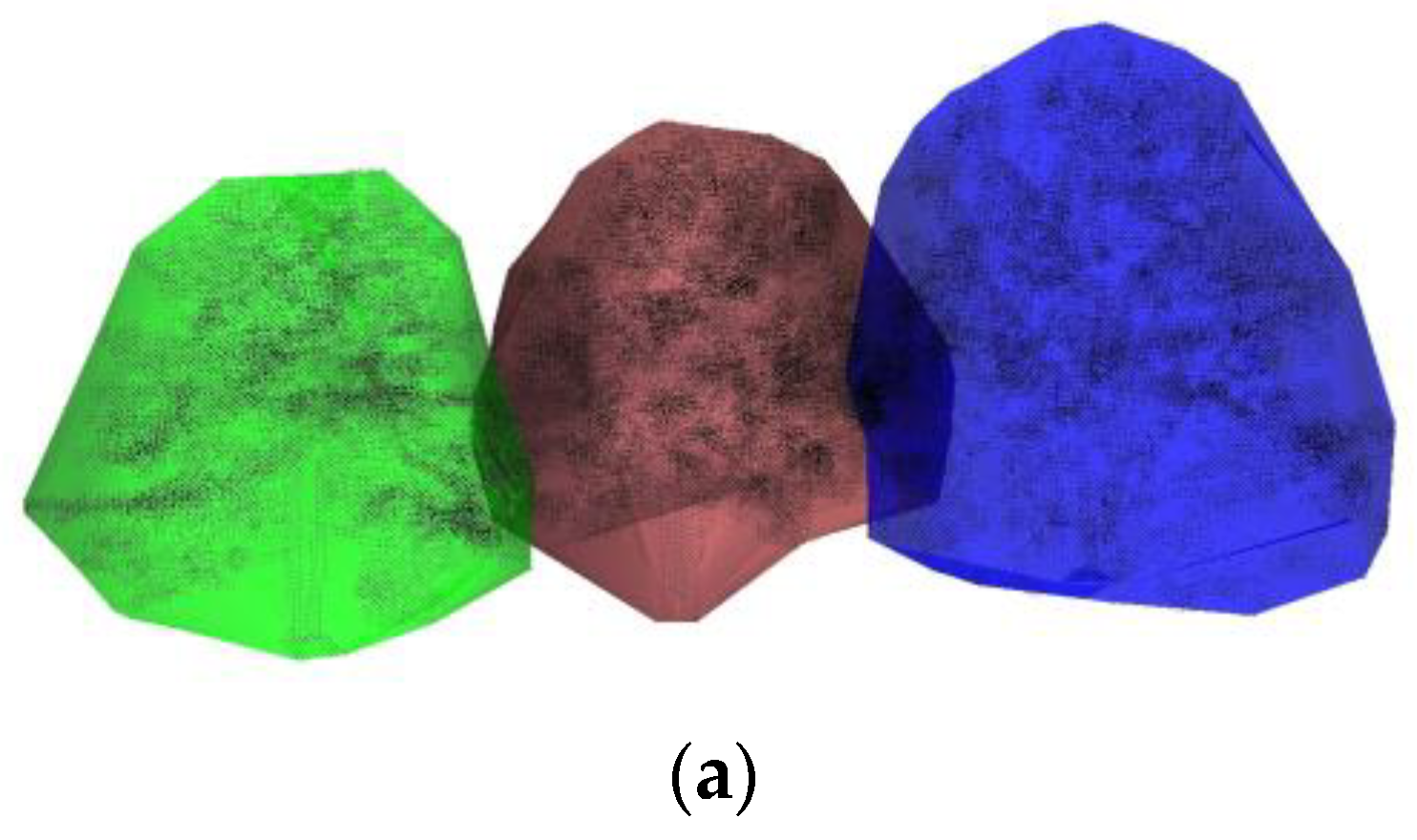
For the four pine trees, we use our method to construct each tree crown separately, as shown in Figure 15. It can be found that the shape of the reconstructed crowns shows a realistic visual effect.

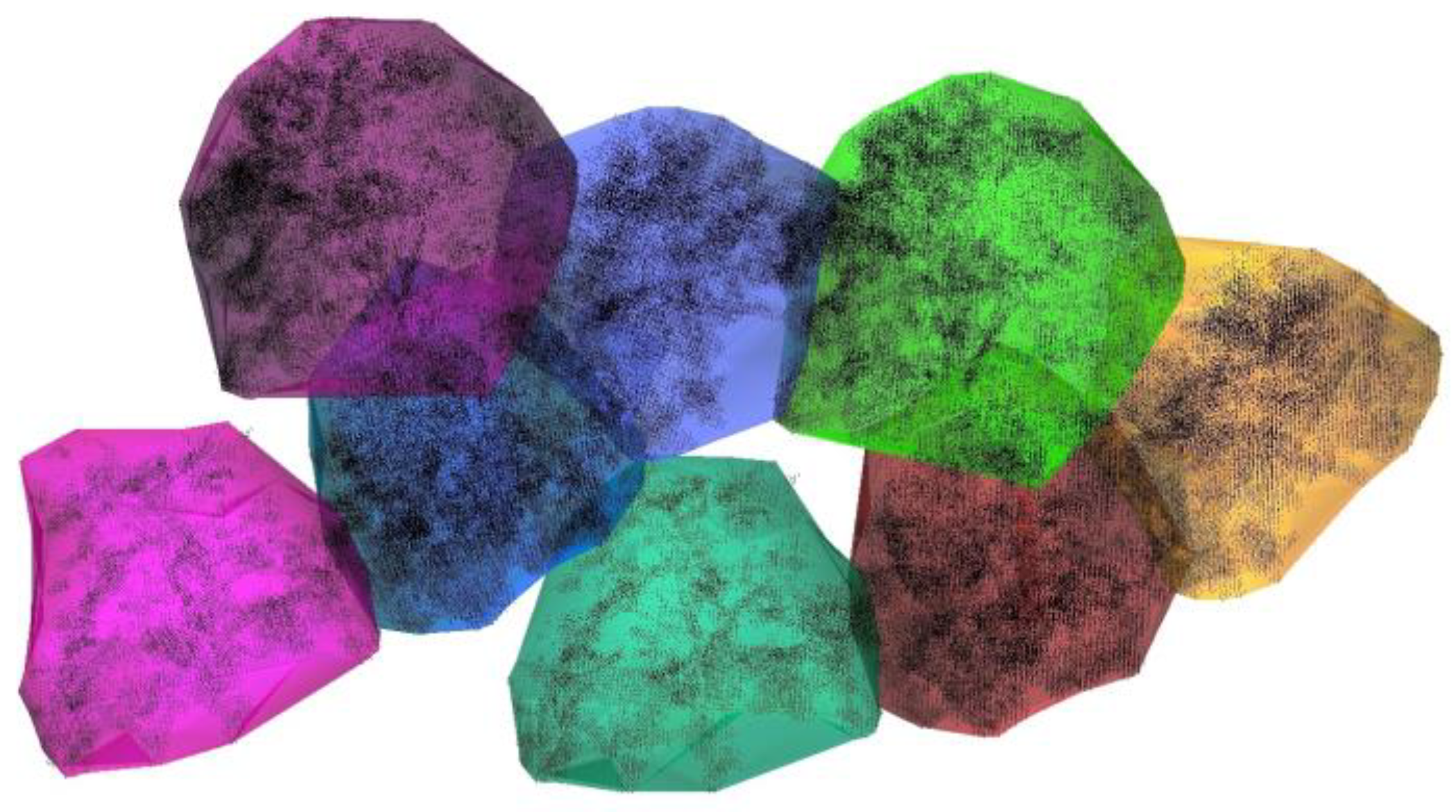
In addition, a small forest, Forest D, built using eight trees, consists of two pieces of Forest C using a rotational transformation and a translational transformation. The picture of the Forest D is shown in Figure 3, and its reconstructed individual tree shape is illustrated in Figure 16.

For the forest RUSH06, we use our method to segment individual trees and reconstruct each tree crown silhouette shape separately. The reconstructed results are displayed in Figure 17.

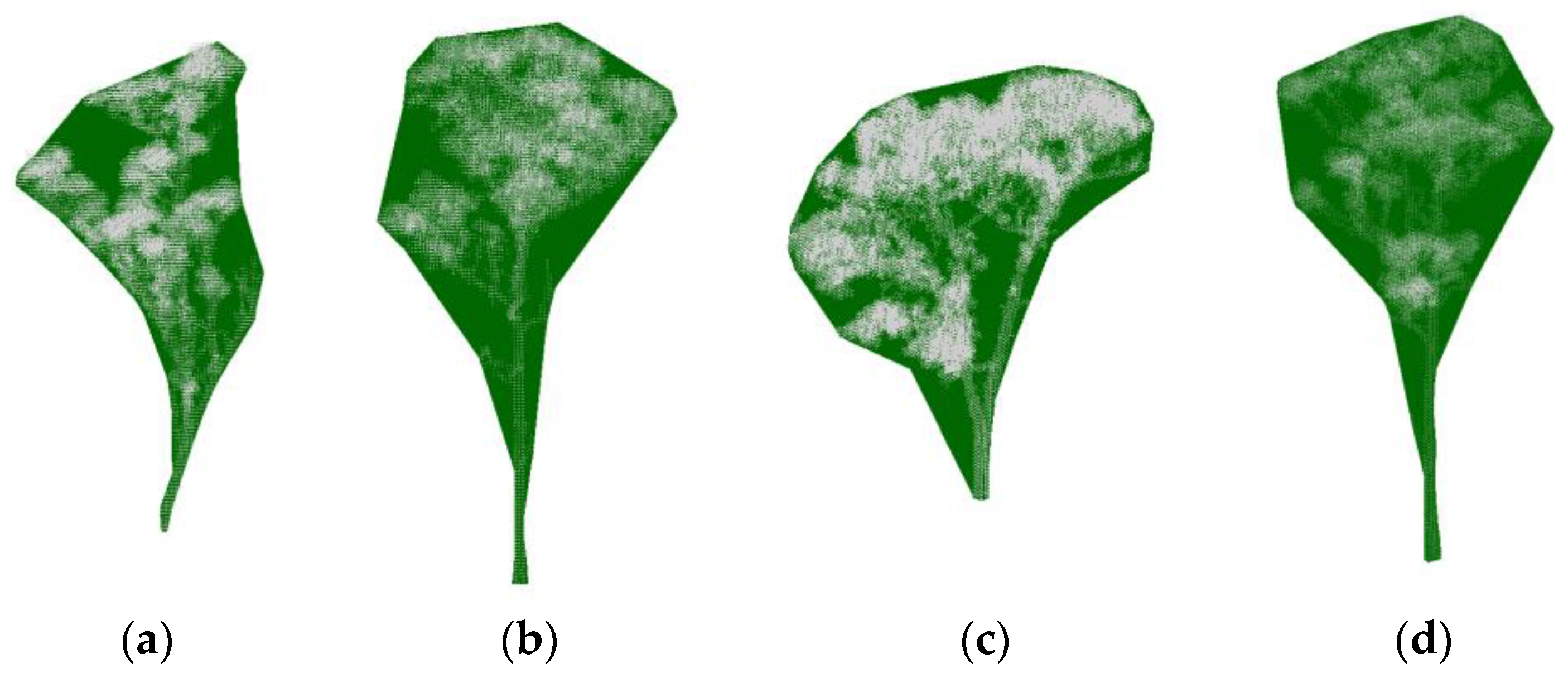
To visually verify the consistency between the tree point clouds and their silhouette surface, the points and their silhouette surfaces of the four trees are shown in Figure 18. It can also be found that the shape of reconstructed crowns shows a realistic visual effect.

3.4. Time Efficiency

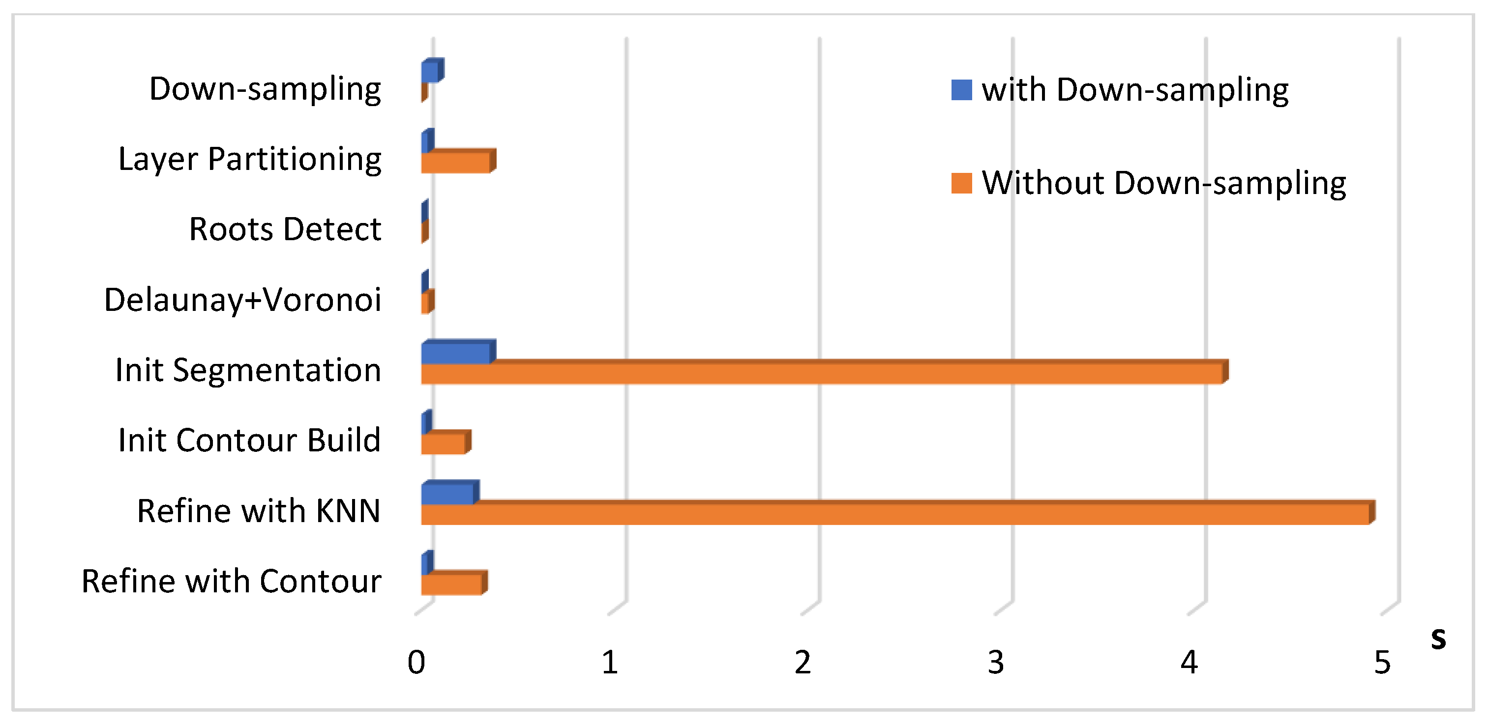
The proposed method adopts down-sampling as the first step of our soft segmentation algorithm, which can significantly improve computing speed in subsequent steps. We use the segmentation experiment of Forest D to evaluate the time cost of each algorithm step when the down-sampling is (or is not) adopted as one preprocessing step, as shown in Figure 19. The running time (unit: s) of all steps using down-sampling is much shorter than that without using down-sampling. The overall running time of the algorithm with or without down-sampling is 0.7959 s and 9.9816 s, respectively.

The running time of each algorithm step of all segmentation experiments is listed in

Table 6. The running time (unit: s) of segmentation experiments of five forest point clouds.

Steps	Forest A	Forest B	Forest C	Forest D	RUSH06
Down-sampling	0.0434	0.0376	0.0479	0.0851	0.7864
Region Growing	0	0	0	0	3.5919
Layer Partitioning	0.031	0.0378	0.0394	0.033	0.1098
Roots Detect	0.0036	0.0041	0.0049	0.0018	0.014
Delaunay + Voronoi	0.0024	0.0022	0.0029	0.0037	0.0176
Init Segmentation	0.0295	0.0279	0.0534	0.3537	0.6606
Init Contour Build	0.0111	0.0108	0.012	0.0214	0.0436
Refine with KNN	0.0777	0.0895	0.1076	0.2674	1.083
Refine with Contour	0.0119	0.0128	0.014	0.0298	0.0697
Total	0.2106	0.2227	0.2821	0.7959	6.3766

. Because the tree crowns in each point cloud, Forest A, Forest B, Forest C, and Forest D, overlap with each other, the step of region growing is not employed, and the time cost is zero. From Table 6, it can be found that a small forest point cloud, for example, when the number of points is about ten million points, can be segmented in several seconds; the two steps region growing and refining with KNN take the most time.

4. Conclusions and Future Work

To address the problem of an apparent artificial segmentation plane between adjacent tree crowns caused by hard segmentation, we, in this paper, propose a soft segmentation algorithm combining KNN with the contour shape constraints. Based on the segmented individual tree point set, the tree crown silhouette surface can be reconstructed with realistic figures, which is beneficial for shape modeling and crown analysis. Experimental results show that the segmentation performance has also been significantly improved in view of three quantitative indicators, Acc, mAcc, and mIoU; the time efficiency of point cloud segmentation has been improved by using down-sampling.

Although the soft segmentation method we propose here provides efficient segmentation of canopy overlay areas and improves speed and accuracy, this method needs more actual data to validate it further. Therefore, one of the future research directions is using the soft segmentation method to test more forest point cloud data, where the overlapping patterns of the canopy are more complex. Hence, the soft segmentation approach here needs to be further expanded. Another promising research direction is destructive laser point cloud data acquisition of forests to obtain accurate canopy shapes that are not accurately measured when they overlap each other. In addition, it is also meaningful to study the relationship between the distance between trees and the shape of the overlapping area of the canopy using this laser scanning point cloud data.

References

1. Budei, B.C.; St-Onge, B.; Hopkinson, C.; Audet, F. Identifying the genus or species of individual trees using a three-wavelength airborne lidar system. Remote Sens. Environ. 2018, 204, 632–647. [Google Scholar] [CrossRef]
2. Ayrey, E.; Fraver, S.; Kershaw, J.A., Jr.; Kenefic, L.S.; Hayes, D.; Weiskittel, A.R.; Roth, B.E. Layer Stacking: A novel algorithm for individual forest tree segmentation from LiDAR point clouds. Can. J. Remote Sens. 2017, 43, 16–27. [Google Scholar] [CrossRef]
3. Hamraz, H.; Contreras, M.A.; Zhang, J. A scalable approach for tree segmentation within small-footprint airborne LiDAR data. Comput. Geosci. 2017, 102, 139–147. [Google Scholar] [CrossRef]
4. Xiao, W.; Zaforemska, A.; Smigaj, M.; Wang, Y.; Gaulton, R. Mean shift segmentation assessment for individual forest tree delineation from airborne lidar data. Remote Sens. 2019, 11, 1263. [Google Scholar] [CrossRef]
5. Ma, Z.; Pang, Y.; Wang, D.; Liang, X.; Chen, B.; Lu, H.; Weinackerm, H.; Koch, B. Individual tree crown segmentation of a larch plantation using airborne laser scanning data based on region growing and canopy morphology features. Remote Sens. 2020, 12, 1078. [Google Scholar] [CrossRef]
6. Liu, Q.; Ma, W.; Zhang, J.; Liu, Y.; Xu, D.; Wang, J. Point-cloud segmentation of individual trees in complex natural forest scenes based on a trunk-growth method. J. For. Res. 2021, 32, 12. [Google Scholar] [CrossRef]
7. Wang, D.; Liang, X.; Mofack, G.I.; Martin-Ducup, O. Individual tree extraction from terrestrial laser scanning data via graph pathing. For. Ecosyst. 2021, 8, 11. [Google Scholar] [CrossRef]
8. Lu, X.; Guo, Q.; Li, W.; Flanagan, J. A bottom-up approach to segment individual deciduous trees using leaf-off LiDAR point cloud data. ISPRS J. Photogramm. Remote Sens. 2014, 94, 1–12. [Google Scholar] [CrossRef]
9. Chen, Q.; Wang, X.; Hang, M.; Li, J. Research on the improvement of single tree segmentation algorithm based on airborne LiDAR point cloud. Open Geosci. 2021, 13, 705–716. [Google Scholar] [CrossRef]
10. Comesaña-Cebral, L.; Martínez-Sánchez, J.; Lorenzo, H.; Arias, P. Individual tree segmentation method based on mobile backpack LiDAR point clouds. Sensors 2021, 21, 6007. [Google Scholar] [CrossRef]
11. Dersch, S.; Heurich, M.; Krueger, N.; Krzystek, P. Combining graph-cut clustering with object-based stem detection for tree segmentation in highly dense airborne lidar point clouds. ISPRS J. Photogramm. Remote. Sens. 2021, 172, 207–222. [Google Scholar] [CrossRef]
12. Li, H.; Zhang, X.; Jaeger, M.; Constant, T. Segmentation of forest terrain laser scan data. In Proceedings of the 9th ACM SIGGRAPH Conference on Virtual-Reality Continuum and Its Applications in Industry, Seoul, Republic of Korea, 12–13 December 2010; ACM: New York, NY, USA, 2010. [Google Scholar]
13. Tang, F.; Zhang, X.; Liu, J. Segmentation of tree crown model with complex structure from airborne LiDAR data. In Proceedings of the 15th International Conference on Geoinformatics, Nanjing, China, 25–27 May 2007; Volume 6752. [Google Scholar]
14. Wang, P.; Xing, Y.; Wang, C.; Xi, X. A graph cut-based approach for individual tree detection using airborne LiDAR data. J. Univ. Chin. Acad. Sci. 2019, 36, 385–391. [Google Scholar]
15. Xiao, W.; Xu, S.; Elberink, S.O.; Vosselman, G. Individual tree crown modeling and change detection from airborne LiDAR data. IEEE J. Sel. Top. Appl. Earth Obs. Remote Sens. 2016, 9, 3467–3477. [Google Scholar] [CrossRef]
16. Robert, M.; Jakub, L.; Theodora, L. Automatic tree crown extraction from uas multispectral imagery for the detection of bark beetle disturbance in mixed forests. Remote Sens. 2020, 24, 4081. [Google Scholar]
17. Ma, K.; Xiong, Y.; Jiang, F.; Chen, S.; Sun, H. A novel vegetation point cloud density tree-segmentation model for overlapping crowns using uav LiDAR. Remote Sens. 2021, 13, 1442. [Google Scholar] [CrossRef]
18. Shahzad, M.; Schmitt, M.; Zhu, X.X. Segmentation and crown parameter extraction of indiviudal trees in an airborne TomoSAR point cloud. In Proceedings of the Copernicus Publications, PIA15+HRIGI15—Joint ISPRS Conference, Munich, Germany, 25–27 March 2015. [Google Scholar]
19. Dong, T.; Zhang, X.; Ding, Z.; Fan, J. Multi-layered tree crown extraction from LiDAR data using graph-based segmentation. Comput. Electron. Agric. 2020, 170, 105213. [Google Scholar] [CrossRef]
20. Novotn, J. Tree crown delineation using region growing and active contour: Approach introduction. Mendel 2014, 2014, 213–216. [Google Scholar]
21. Duan, Z.; Zhao, D.; Zeng, Y.; Zhao, Y.; Wu, B.; Zhu, J. Assessing and correcting topographic effects on forest canopy height retrieval using airborne LiDAR data. Sensors 2015, 15, 12133–12155. [Google Scholar] [CrossRef]
22. Strîmbu, V.F.; Strîmbu, B.M. A graph-based segmentation algorithm for tree crown extraction using airborne LiDAR data. ISPRS J. Photogramm. Remote Sens. 2015, 104, 30–43. [Google Scholar] [CrossRef]
23. Aubry-Kientz, M.; Laybros, A.; Weinstein, B.; Ball, J.G.; Jackson, T.; Coomes, D.; Vincent, G. Multi-sensor data fusion for improved segmentation of individual tree crowns in dense tropical forests. IEEE J. Sel. Top. Appl. Earth Obs. Remote Sens. 2021, 14, 3927–3936. [Google Scholar] [CrossRef]
24. Janoutová, R.; Homolová, L.; Novotný, J.; Navrátilová, B.; Pikl, M.; Malenovský, Z. Detailed reconstruction of trees from terrestrial laser scans for remote sensing and radiative transfer modelling applications. Silico Plants 2021, 3, diab026. [Google Scholar] [CrossRef]
25. Pyysalo, U.; Hyyppa, H. Reconstructing tree crowns from laser scanner data for feature extraction. In Proceedings of the ISPRS Commission III, Symposium 2002, Graz, Austria, 9–13 September 2002. 4p. [Google Scholar]
26. Zhu, C.; Zhang, X.; Hu, B.; Jaeger, M. Reconstruction of Tree Crown Shape from Scanned Data. In Proceedings of the Technologies for E-Learning and Digital Entertainment, Third International Conference, Edutainment 2008, Nanjing, China, 25–27 June 2008; Springer: Berlin/Heidelberg, Germany, 2008. [Google Scholar]
27. Lin, Y.; Hyyppa, J. Multiecho-recording mobile laser scanning for enhancing individual tree crown reconstruction. IEEE Trans. Geosci. Remote Sens. 2012, 50, 4323–4332. [Google Scholar] [CrossRef]
28. Kato, A.; Moskal, L.M.; Schiess, P.; Swanson, M.E.; Calhoun, D.; Stuetzle, W. Capturing tree crown formation through implicit surface reconstruction using airborne LiDAR data. Remote Sens. Environ. 2016, 113, 1148–1162. [Google Scholar] [CrossRef]
29. Calders, K. Terrestrial Laser Scans—Riegl VZ400, Individual Tree Point Clouds and Cylinder Models, Rushworth Forest; Version 1; Terrestrial Ecosystem Research Network (Dataset): Indooroopilly, QLD, Australia, 2014. [Google Scholar] [CrossRef]
30. Fang, H.; Li, H. Counting of plantation trees based on line detection of point cloud data. Geomatics and Information Science of Wuhan University, 22 July 2022, pp. 1–13. [CrossRef]
31. Wang, J.; Li, H. Registration of 3D point clouds based on voxelization simplify and accelerated iterative closest point algorithm. In Artificial Intelligence—CICAI 2021; Lecture Notes in Computer Science; LNAI 13069; Springer: Cham, Switzerland, 2021; pp. 276–288. [Google Scholar] [CrossRef]
32. Al-Rawabdeh, A.; He, F.; Habib, A. Automated feature-based down-sampling approaches for fine registration of irregular point clouds. Remote Sens. 2020, 12, 1224. [Google Scholar] [CrossRef]
33. Yun, T.; Jiang, K.; Li, G.; Eichhorn, M.P.; Fan, J.; Liu, F.; Chen, B.; An, F.; Cao, L. Individual tree crown segmentation from airborne LiDAR data using a novel Gaussian filter and energy function minimization-based approach. Remote Sens. Environ. 2021, 256, 112307. [Google Scholar] [CrossRef]
34. Herbert, E.; Ernst, P.M. Three-dimensional alpha shapes. ACM Trans. Graph. 1994, 13, 43–72. [Google Scholar]
35. Sunil, A.; Theocharis, M.; David, M. Space-time tradeoffs for approximate nearest neighbor searching. J. ACM 2009, 57, 1–54. [Google Scholar]
36. Li, S.; Li, H. Surface reconstruction algorithm using self-adaptive step alpha-shape. J. Data Acquis. Process. 2019, 34, 491–499. [Google Scholar] [CrossRef]
37. Yang, X.; del Rey Castillo, E.; Zou, Y.; Wotherspoon, L.; Tan, Y. Automated semantic segmentation of bridge components from large-scale point clouds using a weighted superpoint graph. Autom. Constr. 2022, 142, 104519. [Google Scholar] [CrossRef]
Figure 1. Laser scan data of 4 pines: (a) Pine A; (b) Pine B; (c) Pine C; and (d) Pine D.
Applsci 13 06228 g001
Figure 2. Three small forest point clouds are built with several trees. The color of a point is related to its y-coordinate and is a pseudo color used only to enhance visual effects. (a) Forest A, trees in line; (b) Forest B, triangular layout; (c) Forest C, quadrangular layout.
Applsci 13 06228 g002
Figure 3. Forest D consists of 8 trees. (a) Front view; (b) top view; Forest C is surrounded by a blue rectangle.
Applsci 13 06228 g003
Figure 4. RUSH06, a laser scan data from the Eucalypt Open Forest [29].
Applsci 13 06228 g004
Figure 5. The down-sampling results with different sampling intervals (up: 0.15; down: 0.25) are illustrated using the point cloud of Forest A. (a) The sampling interval is 0.15; (b) top view of (a); (c) the sampling interval is 0.25; (d) top view of (c).
Applsci 13 06228 g005
Figure 6. The rough segmentation results of RUSH06 using the region growth algorithm. Different groups use different colors.
Applsci 13 06228 g006
Figure 7. The best segment line detection in the hard segmentation algorithm; (a) segment plane; (b) rough cell of an individual tree.
Applsci 13 06228 g007
Figure 8. The individual tree identification with the hard segmentation. The three vertices of the black triangle show the positions of three roots. (a) The segmentation result of Forest B; (b) the top view of (a).
Applsci 13 06228 g008
Figure 9. The pending region is introduced to the hard segmentation algorithm.
Applsci 13 06228 g009
Figure 10. Key steps and results of refined segmentation. (a) Generating horizontal layers; (b) building the contours of all layers; (c) refining by KNN and contour constraints; (d) one representative layer of (b); (e) refined contour and classification of (d).
Applsci 13 06228 g010
Figure 11. The individual tree identification with the soft segmentation algorithm. (a) The segmentation result of Forest B; (b) the top view of (a).
Applsci 13 06228 g011
Figure 12. The individual tree of Forest A partitioning using the soft segmentation method.
Applsci 13 06228 g012
Figure 13. The individual tree identification using the soft segmentation method. The green lines on the ground show the edges of the Voronoi graph, which is constructed using the root positions as sites. (a) The segmentation result of Forest C; (b) the segmentation result of Forest D.
Applsci 13 06228 g013
Figure 14. The segmentation results of RUSH06 using different segmentation methods. (a) Hard segmentation; (b) soft segmentation without precession; (c) soft segmentation with precession; (d) another view of (c).
Applsci 13 06228 g014
Figure 15. The reconstructed shapes of three small forest point clouds in Figure 2. (a) Reconstructed individual tree shapes of Forest A; (b) reconstructed tree shapes of Forest B; (c) reconstructed tree shapes of Forest C.
Applsci 13 06228 g015aApplsci 13 06228 g015b
Figure 16. Reconstructed individual tree shape of Forest D in Figure 3.
Applsci 13 06228 g016
Figure 17. The reconstructed individual tree crowns with the random coloring of RUSH06. (a) A font view; (b) the top view of (a).
Applsci 13 06228 g017aApplsci 13 06228 g017b
Figure 18. The reconstructed individual tree crowns from RUSH06. (a) Tree 1; (b) Tree 2; (c) Tree 3; (d) Tree 4.
Applsci 13 06228 g018
Figure 19. Comparison of the time cost of each algorithm step when the down-sampling is (or is not) adopted as one step of preprocessing.
Applsci 13 06228 g019