Article

BILSTM-Based Deep Neural Network for Rock-Mass Classification Prediction Using Depth-Sequence MWD Data: A Case Study of a Tunnel in Yunnan, China

1
State Key Laboratory of Geomechanics and Geotechnical Engineering, Institute of Rock and Soil Mechanics, Chinese Academy of Sciences, Wuhan 430071, China
2
University of Chinese Academy of Sciences, Beijing 100049, China
3
School of Civil Engineering and Transportation, South China University of Technology, Guangzhou 510641, China
*
Author to whom correspondence should be addressed.
Appl. Sci. 2023, 13(10), 6050; https://doi.org/10.3390/app13106050
Submission received: 28 March 2023 / Revised: 9 May 2023 / Accepted: 10 May 2023 / Published: 15 May 2023
(This article belongs to the Section Civil Engineering)

Abstract

:
Measurement while drilling (MWD) data reflect the drilling rig–rock mass interaction; they are crucial for accurately classifying the rock mass ahead of the tunnel face. Although machine-learning methods can learn the relationship between MWD data and rock mechanics parameters to support rock classification, most current models do not consider the impact of the continuous drilling-sequence process, thereby leading to rock-classification errors, while small and unbalanced field datasets result in poor model performance. We propose a novel deep neural network model based on Bi-directional Long Short-Term Memory (BILSTM) to extract information-related sequences in MWD data and improve the accuracy of the rock-mass classification. Two optimization modules were designed to improve the model’s generalization performance. Stratified K-fold cross-validation was used for model optimization in small and unbalanced datasets. Model validation is based on the MWD dataset of a highway tunnel in Yunnan, China. Multiple metrics show that the prediction ability of the network is significantly better than those of a multilayer perceptron (MLP) and a support-vector machine (SVM), while the model exhibits an improved generalization performance. The accuracy of the network can reach 90%, which is 13% and 15% higher than the MLP and SVM, respectively.

1. Introduction

Tunnel engineering is a crucial part of transportation engineering. Mountainous areas are characterized by significant terrain-height differences, strong tectonic activities, and complex and changeable hydrogeological environments, which can result in great safety hazards during tunnel construction [1,2]. Therefore, it is necessary to evaluate the surrounding rock conditions in front of the tunnel face during tunnel constructions; this can be done through advanced geological forecasting and can prevent potential geological disasters [3,4,5], such as large surrounding rock deformation, landslides, karst collapse, water and/or mud inflow [6,7,8].
MWD technology is used for advanced geological forecasting or rock mass classification. Many scholars have conducted extensive research on this topic and found correlations between the drilling parameters of the drilling rig and the physical and mechanical properties of the rock and soil. If the surrounding rock conditions in front of the face can be evaluated and classified by monitoring and analyzing MWD data, advanced geological forecasting can become more efficient and its cost can be reduced.
Somerton and Tot studied the relationships among the drilling parameters of rotary drilling rigs, drilling energy, and rock drillability through laboratory experiments [9]. Hamelin et al. developed the ‘Enpasol’ digital recorder for recording the drilling parameters of the drilling rig and classifying the rock and soil [10]. Schunnesson considered percussion drilling parameters and the variability between them and predicted the rock-quality designation (RQD) during tunnel excavation [11]. Yue et al. improved the monitoring method of the drilling rate, proposed a fast and intuitive time series analysis method of the space–time data of the drilling process, and suggested that the change in formation could be predicted according to the change in the penetration rate of drilling [12]. Wang et al. set up an indoor rock-mass digital drilling test platform to investigate the relationships between the drilling parameters and rock properties based on a polycrystalline diamond compact (PDC) bit [13]. Liang et al. proposed a probability-classification method for formation recognition based on Bayesian principles [14]. Many assumptions and linear fitting relationships for rock-formation classification or rock-mass classification predictions based on MWD data were used in traditional theoretical methods [15]; these are inconsistent with the complex variability of the actual drilling process in the field and the nonlinear relationships between parameters. In recent years, some scholars have introduced machine learning in the field of rock-mass identification [16,17]; such methods can determine the laws between multiple variables from the data and provide the required results when the process mechanism is not clear [18,19]. LaBelle et al. used the neural network method to classify lithologies based on laboratory drilling experimental data [20]. Gao et al. used an SVM to build a relationship model between the parameters of the PDC bit while drilling and the rock-mass uniaxial compressive strength (UCS) [21]. These studies demonstrate that machine learning can effectively identify the properties of rock and soil based on drilling parameters using simple models and less noisy indoor drilling experiment data. Ameur-Zaimeche et al. used different machine-learning methods to predict porosity with reservoir-associated gas using gas-while-drilling data [22]. Kadkhodaie-Ilkhchi et al. based on the fuzzy logic (FL) algorithm [23], Fang et al. based on the MLP, Klyuchnikov et al. and Romanenkova et al. based on the DT ensemble learning conducted formation-lithology recognition [24,25,26], applied machine learning methods in practical engineering with a large amount of noisy data. Although current machine-learning algorithms can achieve good prediction results, several shortcomings persist: (1) Drilling is a continuous process; however, these studies only use the drilling data corresponding to the position to classify the rock class at a certain depth during the drilling process. Gupta et al. demonstrated through their research that considering the information contained in the sequence can improve the accuracy of results [27]. (2) Datasets obtained in practice are small and prone to overfitting, thereby impacting the prediction effect. (3) Most studies use accuracy as model performance evaluation metric, but the proportions of the surrounding rocks of different classes in an actual project vary greatly. For such unbalanced datasets, a single evaluation metric may incorrectly evaluate model performance.
To address the aforementioned issues, this study proposes a machine-learning method with BILSTM as the core, using depth-sequence MWD data to classify rock-mass classes in real-time. (1) The BILSTM was used to fully consider the influence of depth-sequence MWD data on rock-classification results. Information related to the surrounding rock class were extracted in both the forward and reverse directions. (2) Stratified K-fold cross-validation determined the optimal model in a small and unbalanced dataset to avoid overfitting. The voting mechanism was designed to avoid random effects and misidentification in special circumstances, while the random window-selection mechanism was devised to enhance the model’s generalization ability. (3) Multiple evaluation metrics were used for unbalanced datasets to provide a comprehensive evaluation of the model’s performance from various perspectives. This method was verified using MWD data from a highway tunnel in Yunnan Province, China.

2. Dataset Establishment and Preprocessing

2.1. Dataset Source

MWD data were collected from various sensors during drilling on the KOKEN RPD-180CBR multifunction rig. The monitored parameters included drilling time, depth, torque, number of rotations, thrust, percussive force, beat number, water-supply rate, water-supply pressure, drainage rate, and drainage pressure. In addition, the penetration rate of drilling, penetration energy, EV energy, and ELT were calculated using the monitored parameters. Surrounding rock classes were also recorded. The recorded major drilling parameters are listed in Table 1; these data were recorded at fixed depth intervals to compose the depth-sequence MWD data. The typical monitoring results of some drilling parameters are shown in Figure 1.

2.2. Key Drilling-Parameter Selection

Different drilling parameters contain different information and exhibit different correlations with the surrounding rock classes. To reduce the feature dimensions and improve the analysis efficiency, it is necessary to retain the parameters exhibiting high correlations and filter the parameters exhibiting low correlations with the surrounding rock classes. Because the surrounding rock classes and drilling parameters are related to categorical variables and do not belong to the bivariate normal distribution, the Kendall coefficient [28] was used to evaluate the correlations between drilling parameters and the surrounding rock classes.
The Kendall coefficient evaluates the correlation between the two random parameters. In this study, the Taub in Kendall’s method was used to evaluate the correlations between the parameters while drilling and the surrounding rock classes; the parameters while drilling that exhibited low correlations with the surrounding rock classes were excluded from the features. Assuming that X represents a parameter while drilling variable and Y represents a rock-class variable, the calculation of Taub is as follows:
Tau b ( X , Y ) = N c N d ( n 0 n 1 ) ( n 0 n 2 )  
n 0 = n ( n 1 ) 2  
n 1 = i t i ( t i 1 ) 2  
n 2 = j u j ( u j 1 ) 2  
where n is the number of elements contained in the variable, n 0 is the total number of element pairs, N c is the number of element pairs in the same order, N d is the number of element pairs in the reverse order, and n 1 and n 2 are the number of the same element pairs in X and Y, respectively.
The Taub value ranges between −1 and 1: The closer it is to 1, the greater the positive correlation between X and Y; the closer it is to −1, the greater the negative correlation between X and Y; and the closer it is to 0, the weaker the correlation between X and Y. Simultaneously, the p value is calculated with Taub, reflecting the significance level of the correlation; as shown in Table 2, if p > 0.05, Taub is unreliable. If p < 0.05 or p < 0.01, Taub is reliable.

2.3. Dataset Division

In this study, the surrounding rock was classified according to the surrounding rock conditions revealed by excavation. While maintaining one-to-one correspondence between the depth-sequence MWD data and surrounding rock classes, and eventually establishing the MWD dataset for the prediction of the surrounding rock class, the dataset was divided into a training set and a test set.
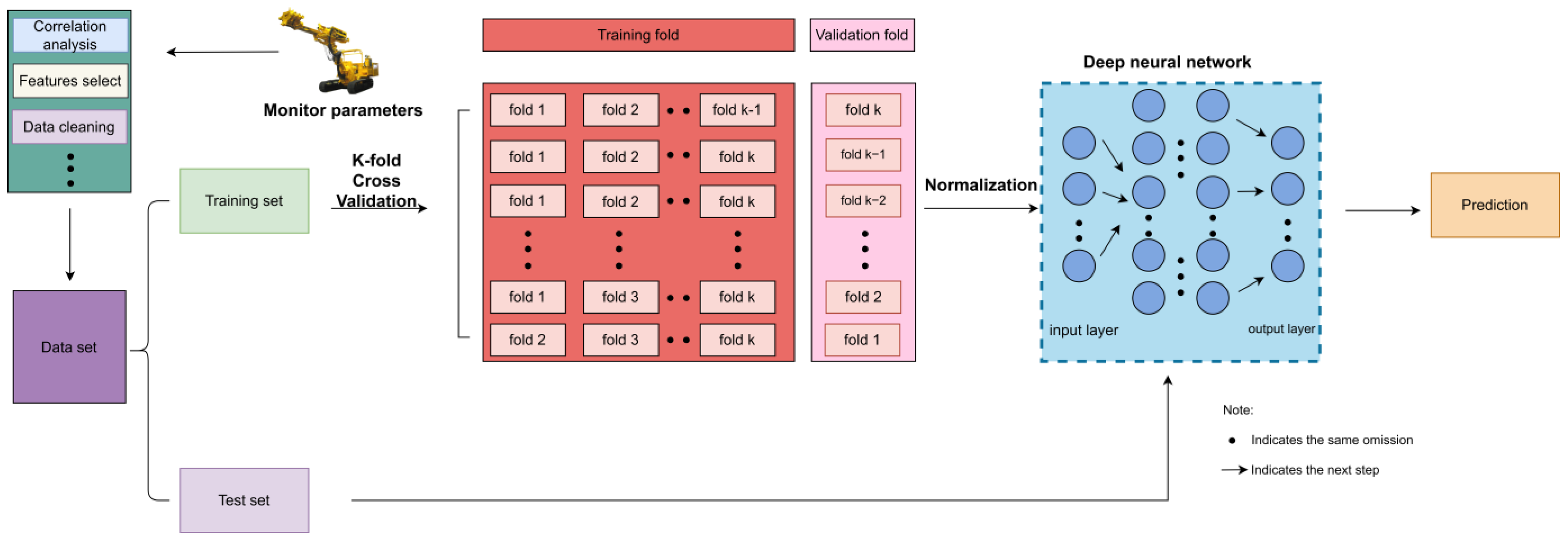
For machine learning, the data determines the upper limit of the model [29,30]. Datasets obtained in practice are usually small and unbalanced, thereby resulting in overfitting; therefore, training the optimal model with limited data while avoiding overfitting is key. Here, the stratified K-fold cross-validation method was used to divide the training set into K parts, of which K − 1 parts were used for model training and one part was used as a validation set. The validation set was not involved in training and was used for cross-cycle validation in the model, i.e., cycling K times to adjust the parameters and evaluate the model. The workflow is shown in Figure 2. Regarding the unbalanced distribution of samples of different rock classes in the dataset, random division may aggravate the unbalance; hence, the stratification method was used to pass the labels of the rock classes in the division and ensure that the proportions of samples of different rock classes in the training and validation sets are the same as that of the original data, thereby reducing adverse effects.

3. BILSTM-Based Deep Neural Network Rock-Mass Classification Method

This section introduces the proposed BILSTM-based deep neural network, including an introduction to the role of each component, the overall network structure, and the evaluation metrics.

3.1. Deep Neural Network Structure

3.1.1. BILSTM Neural Network

The essence of predicting the class of the surrounding rock from the MWD data is a nonlinear classification problem based on the characteristics of the drilling parameters. Drilling the rock mass with the drilling rig is a continuous process; hence, the depth-sequence of the MWD data contains rich and important information. Rock-class prediction based only on the drilling parameters at a certain time or depth is one-sided; considering the influence of the preceding and following depth-series data is also essential for making a comprehensive evaluation.
BILSTM is a variant of long short-term memory (LSTM); it is built from two LSTM networks in opposite directions and can learn the information contained in a depth-sequence by combining the effects of the preceding and following depth-sequence data through bidirectional transfer.
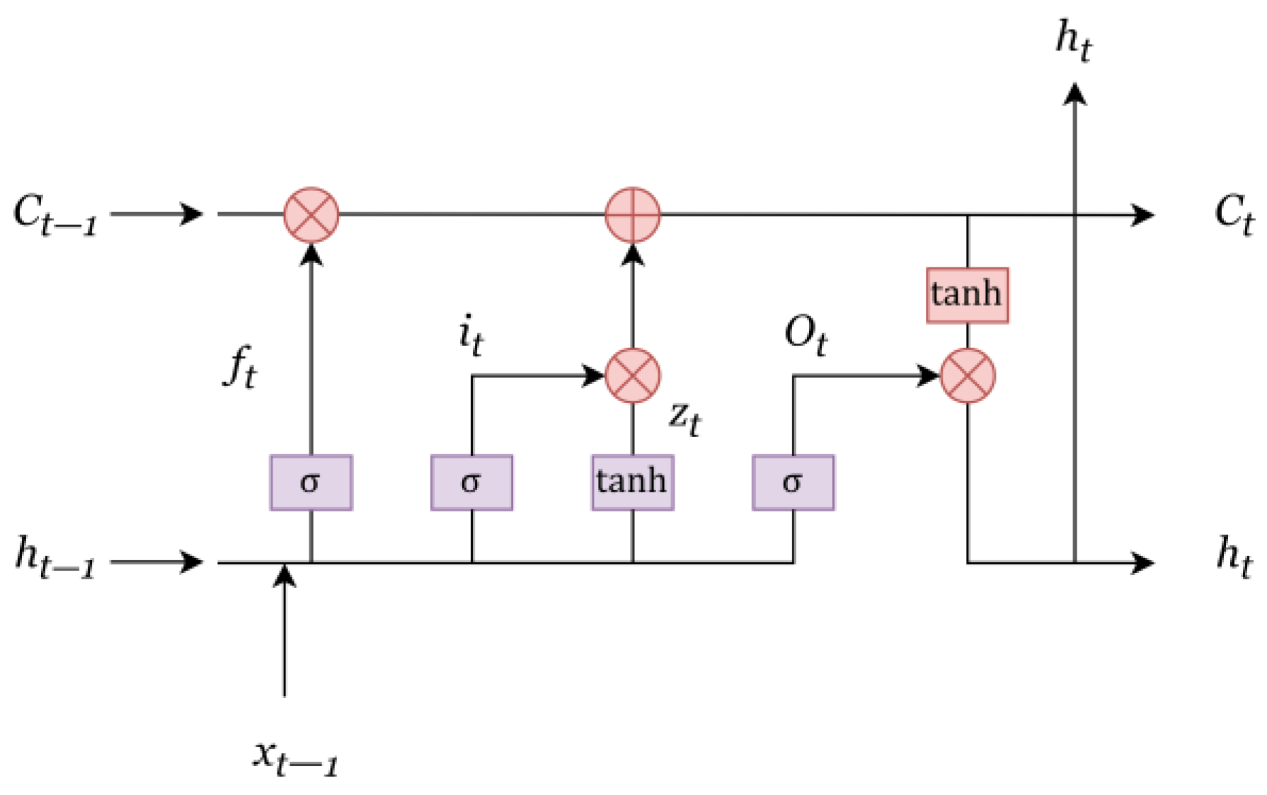
The LSTM neural network was proposed by Hochreiter and Schmidhuber [31] and its structure is illustrated in Figure 3; it adds input, forget, and output gates to the RNN. In this way, disturbing information is eliminated, and the recursive processing of data is selectively performed based on the time or space sequences, thereby solving the problem of gradient disappearance or gradient explosion caused by the traditional RNN. The parameters of the input, forget, and output gates ( i t , f t , and O t , respectively) are updated according to Equations (5)–(10) in the following manner.
Input   values :   Z t = t a n h ( W z [ h t 1 , x t ] + b z )
Input   gates :   i t = σ ( W i [ h t 1 , x t ] + b i   )
Forget   gates :   f t = σ ( W f [ h t 1 , x t ] + b f )
Cells :   C t = f t · C t 1 + i t · Z t
Output   gates :   O t = σ ( W o [ h t 1 , x t ] + b o   )
Outputs :   h t = O t · t a n h   · C t
where tanh is an activation function, σ denotes the sigmod activation function, W denotes the weights, and b denotes the bias.
The values calculated by input, forget, and output gates are all mapped at the (0, 1) interval by the sigmoid function: the closer the value is to 1, the more information is retained; the closer the value is to 0, the more information is rejected.
As shown in Figure 3, the LSTM can only be passed unidirectionally along the sequence direction, i.e., only the influence of the pre-sequence test data can be considered. To consider simultaneously the impact of both the pre- and post-sequence test data, it is necessary to build a BILSTM network with two LSTM networks in opposite directions.
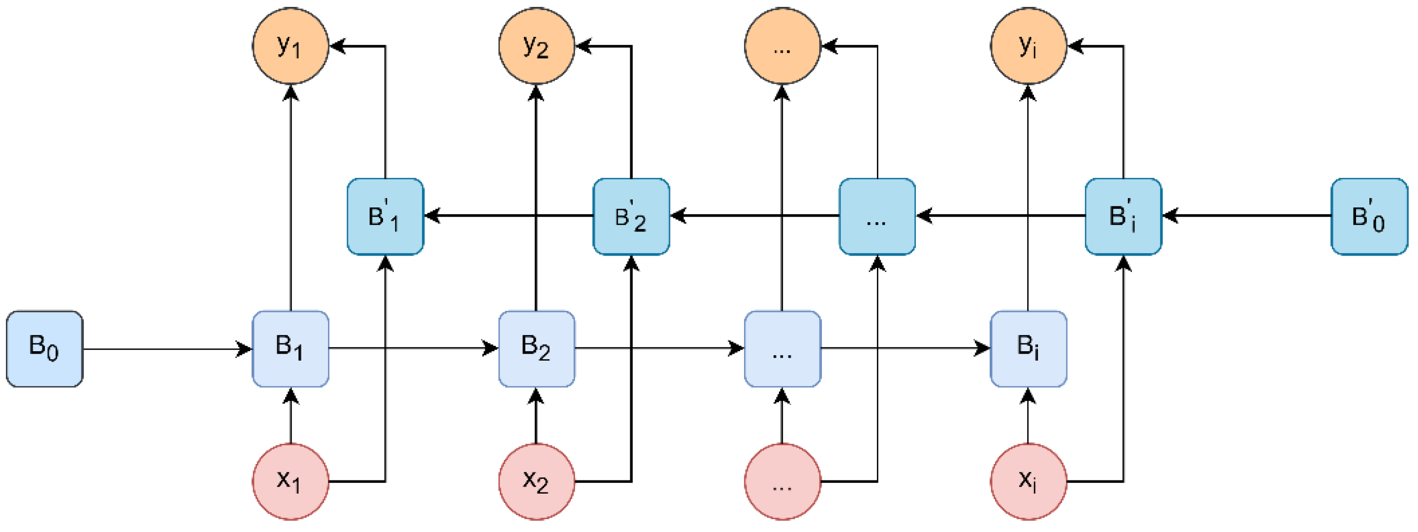
The BILSTM structure is shown in Figure 4; it can combine the pre- and post-sequence information of the current sequence in the output. There are two hidden values, namely B and B′ associated with the sequence in the BILSTM: B is involved in the forward calculation, and   B i is involved in the reverse calculation. The eigenvector x i = ( x 1 , x 2 . , x i ) is connected to the hidden layer through the input layer and B i = f ( A B i + Z   B i + 1 ) and   B i = f ( A B i + 1 + Z B i ) , while subsequently connecting to the output of the next layer, i.e., y i = g ( C B i + C B i ) . This means that for forward computation, B i of the hidden layer is determined by the previous and current sequences, and for reverse computation, B i of the hidden layer is determined by the next and current sequences. The output of each cell in the BILSTM sample is passed through the same number of hidden states; hence, the effect of the information contained in the depth-sequence data in the sample is considered.

3.1.2. Fully Connected Layer

The fully connected layer (FC), in which all neurons in a certain layer are fully connected to all neurons in the previous layer, is essentially a linear transformation from one parameter space to another through operations such as lift, translation, and rotation, and is capable of integrating class-distinct local information and highly purified parameters.
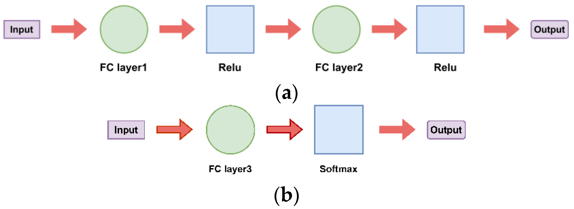
The designed deep neural network has three fully connected layers, of which the first two layers are set before the BILSTM layer (Figure 5a). The activation function is the ‘Relu’ function; it purifies the rock-class information for BILSTM learning, and its output is used as BILSTM-layer input.
The final layer is located after the BILSTM layer (Figure 5b). The activation function is the ‘Softmax’ function; it outputs the BILSTM-prediction result in the form of probability.

3.1.3. Window Selector and Voter

The BILSTM network must consider the window size, i.e., the extent to which the rock mass at a certain depth to be predicted is affected by the pre- and post-sequence depth MWD data. In this study, the initial sample window size was set to 40 cm for each BILSTM cycle, while considering the influence of 20 depth-sequences for predicting the surrounding rock class.
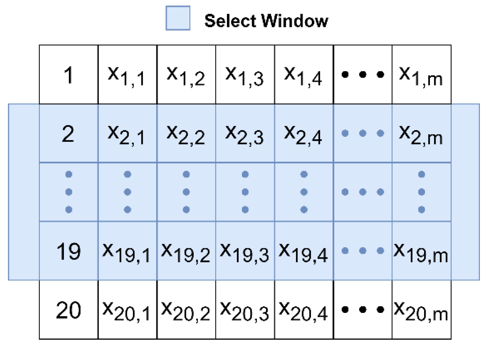
To avoid model overfitting, while improving the generalization of the neural network, we designed a window-selector module with random window selection within the default sample window, as shown in Figure 6. Under the initial sample window, small windows are randomly generated according to the depth-sequence for the BILSTM cycle, so that different information can be learned even if the samples are the same, thereby greatly improving the generalization.
To avoid the data collected at a certain depth being affected by the random effects of site construction and special circumstances that may lead to misclassification, a ‘Voter’ module was designed for the hidden-state outputs at different depths; the voter is shown in Equation (11). The results of each BILSTM unit’s hidden-layer output undergo fully connected Softmax activation, and the prediction results are mapped at the [0, 1] interval by the Softmax function to obtain the predicted rock-class probability. The rock class with the highest probability within the sample circulation window is taken as the final prediction result by the voter.
Vote ( n ) = { I ,   i f   n I = m a x ( n ) II ,   i f   n II = m a x ( n ) III ,   i f   n III = m a x ( n ) IV ,   i f   n IV = m a x ( n ) V ,   i f   n V = m a x ( n )
where n denotes the set of rock-mass class probabilities output by the BILSTM network in the selection window, and n I   to   n V represent the probabilities of different rock-mass classes.

3.1.4. BILSTM-Based Deep Neural Network Structure Design

Considering the influence of pre- and post-sequence MWD data on rock-mass classification, we designed a deep neural network with BILSTM as the core, as shown in Figure 7, supplemented by a fully connected layer to extract information. Batch normalization (BN) solves the internal covariate shift (ICS) problem and improves the model prediction performance [32]. The designed window selector facilitates learning more information and improves the model’s generalization performance, while avoiding overfitting. The rock-class probability is output through the classifier module and the final prediction result is obtained through the ‘Voter’ module to ensure the accuracy of rock classification.
The training and prediction processes of the neural network require taking a sample with a size of (n, m), where n is the random window size of the window selector and m is the number of parameters, from the dataset. First, n eigenvectors with sizes of m are input into the two fully connected layers in turn; at the two fully connected layers, the activation function ‘Relu’ performs operations such as dimension reduction, rotation, translating, etc., thereby purifying the information related to the rock classes, and outputs (n, k) samples, i.e., n vectors with sizes of k, where k is the number of neurons in the output layer of the fully connected layer. It should be noted that the two fully connected layers share weights in a training batch, meaning that data at each depth in the training batch pass through the fully connected layer with the same weight. Next, the (n, k) samples are input into the BILSTM hidden layer, and the information related to the depth-sequence in the learning samples is learned through bidirectional information transfer. Finally, the BILSTM output is passed into the last fully connected layer, whose activation function ‘Softmax’ obtains the rock-class probability; the final prediction result is obtained through ‘Voter’.

3.2. Evaluation Metrics

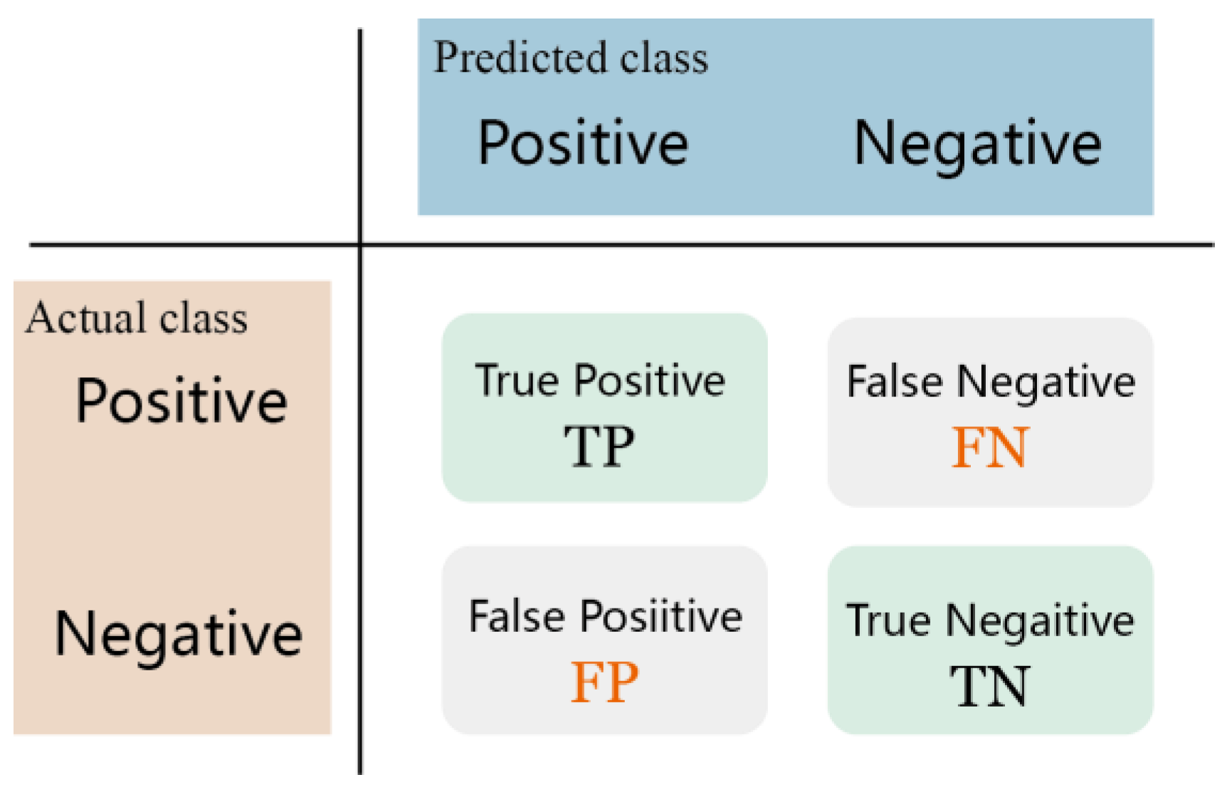
Accuracy is the most intuitive and commonly used metric for assessing model performance; however, it tends to ignore the effects of unbalanced datasets and skews toward the majority class of the sample, thereby resulting in incorrect evaluations [33]. Therefore, to accurately evaluate the model’s predictive performance for unbalanced samples from different perspectives, we used the accuracy, precision, recall, F1 values, and area under curve (AUC) of the receiver operating characteristic curve (ROC) to evaluate the model. These evaluation metrics are based on the confusion matrix shown in Figure 8 and classify the prediction results into four cases.
All of the above evaluation metrics are used for evaluation in the binary classification, and the first four are calculated as follows:
Accuracy = T P + T N T P + T N + F P + F N  
Precision = T P T P + F P  
Recall = T P T P + F N  
F 1 = 2 × Recall × Precision Precision + Recall
Rock-mass classification is a multiclassification problem that can be viewed as a multiple binary classification problem. Because of the unbalance rock-mass percentages in each class, we used the weight-average method to evaluate the overall performance of the model as follows:
Accuracy overall = s c / s  
Precision overall = i = 1 O Precision i w i  
Recall overall = i = 1 O Recal i w i    
F 1 overall = i = 1 O F 1 i w i  
Parameter s represents the total number of samples, s c represents the number of correctly predicted samples, w is the ratio of samples of class i to the total number of samples, Precision i , Recal i , and F 1 i represent the precision, recall, and F 1 values of the rock in class i , respectively.
We used the ROC curve and its corresponding AUC for the binary classification problem. To solve multiclassification problems and evaluate the performance of the model, we used the macro- and micro-average ROCs improved on the basis of ROCs and their corresponding macro- and micro-average AUC values, where the AUC represents the area under the ROC. The closer the value was to 1, the higher the model performance; the closer the value was to 0, the lower the model performance.

4. Engineering Case Application

4.1. Project Overview

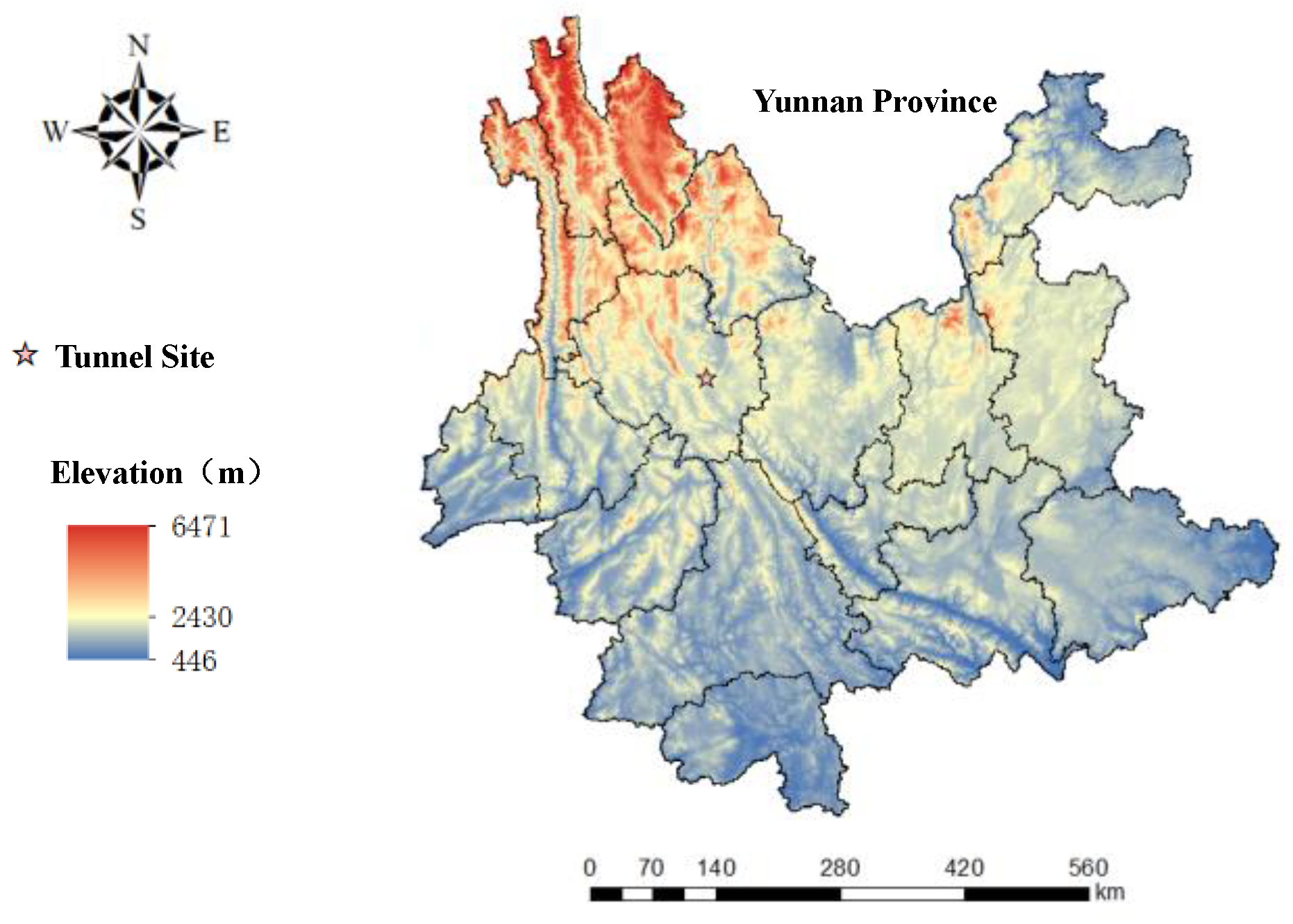
The tunnel is located in Yunnan, China, as shown in Figure 9. The left side starts and ends at pile numbers K281 + 506 and K289 + 090, respectively, and is 7560 m long; the right side starts and ends at pile numbers K281 + 530 and K289 + 103, respectively, is 7597 m long, and passes through 11 fault fracture zones. The geological setting of the tunnel-site area is shown in Figure 10, with various adverse geological bodies being widely distributed along the tunnel route.
Due to the inaccurate classification of surrounding rock in the early stage of construction, the construction excavation disturbed the weak surrounding rock, causing large deformation of the vault, followed by landslide and water and mud inflow, which seriously affected the construction (Figure 11).
To reduce the occurrence of geological hazards, detect the distributions of adverse geological bodies, predict the classes of surrounding rocks in front of the tunnel face, and ensure the safety of tunnel construction, the KOKEN RPD-180CBR multifunctional drilling rig was used to conduct advance drilling and record MWD data in depth-sequence for the section from YK282 + 084.5 to YK282 + 501.0 on the right.
The advance drilling started on 16 June 2018 and ended on 11 December 2018, with a total of 10 advanced boreholes being used for forecasting the 416.5-m rock mass, while recording a total of 27,607 sets of data as well as the corresponding surrounding rock classes. According to the ‘Specifications for Design of Highway Tunnels Section 1 Civil Engineering, China’ [34], China, the surrounding rock classes were III, IV, and V. The drilling dataset was constructed according to the method described in this study, and the BILTSM deep neural network model was used to train the drilling dataset and predict the surrounding rock classes.

4.2. Dataset Creation

The initial MWD data contains 11 parameters, of which 10 are drilling parameters and the other is rock class. The correlation between these parameters were analysed by Kendall coefficient and the key drilling parameters were selected by the Taub value; the results are shown in Table 3, where the p-values are less than 0.05, i.e., the results are reliable. Table 3 shows that the parameters with higher positive correlations with the surrounding rock classes are EV and ELT, and those with higher negative correlations with the surrounding rock classes are drilling speed and torque. This indicates that when the rock integrity is good, the penetration rate of drilling is low and the energy required to break the rock mass is high, which is in line with the actual situation. As the absolute Taub values of the rotation speed, water supply rate, and water supply pressure were less than 0.1, these three parameters were excluded. The Taub values of the penetration energy and beat per minute were 1.0, while the Taub values of EV and ELT were 0.9, with high positive correlations among the parameters. To avoid parameters with high correlations interfering with each other during training, beats per minute and ELT were also excluded. The selected key parameters included the penetration rate of drilling, torque, thrust, penetration energy, and EV energy.
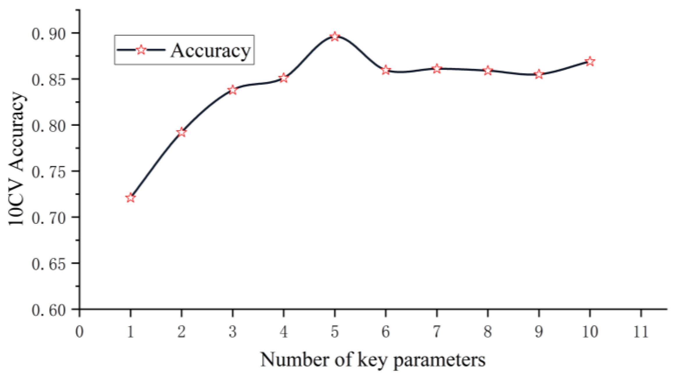
The subsequent optimal deep neural network model with optimal hyperparameters was utilized to develop the 10-fold cross-validation mean accuracy with different numbers of key drilling parameters (Figure 12). The highest accuracy was achieved for the five key drilling parameters, which were selected by Kendall coefficient. The result illustrates the rationality of the key parameters selection method.
The abnormal values of the 27,607 sets of data were removed. Finally, data were min–max normalized. Because of the need for storing rock classes as variables, a one-hot encoding form was used to encode N states with N-bit status registers, representing classes III, IV, and V as (0, 0, 1), (0, 1, 0), and (1, 0, 0), respectively.
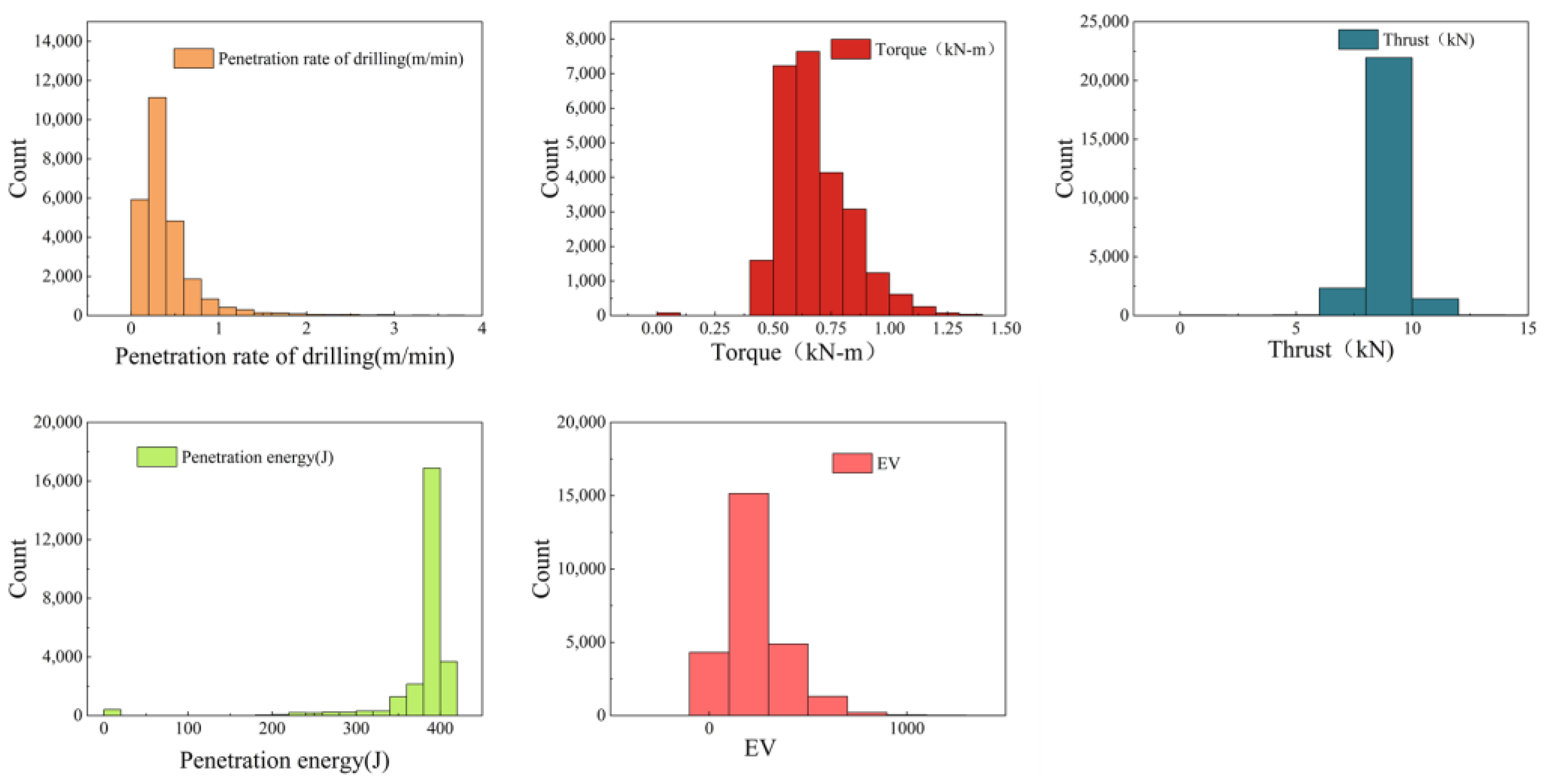
The MWD dataset was packaged as a sample of 20 depth-sequences to obtain a total of 1300 samples and 26,000 sets of data, with a significant imbalance in the percentage of each class of surrounding rocks, as shown in Figure 13a. The data of the first nine advanced drilling holes were divided into the training set, and the data of the last hole was divided into the test set. The training set contained 1200 samples and 24,000 sets of data; the proportion of each rock class are shown in Figure 13b (from III to V are 60.25% (723 samples, 11,460 sets), 23.92% (287 samples, 5740 sets), and 15.83% (190 samples, 3800 sets), respectively). In the training set, 10-fold cross-validation was performed in a ratio of 9:1. As the dataset was unbalanced, the stratified 10-fold method was used to pass the information on the rock-class labels when dividing the dataset to ensure that the proportions of samples of different rock classes in the validation set were the same as those of the original samples. The test set contained 100 samples and 2000 sets of data; the proportion of each rock class are shown in Figure 13c (from III to V are 55% (55 samples, 1100 sets), 27% (27 samples, 540 sets), and 18% (18 samples, 360 sets), respectively). This operation was used to establish the drilling dataset; it can be seen that the proportions of each rock class in the dataset, training set, and test set are roughly consistent. The statistical analysis of the training set and test set are shown in Table 4 and Table 5, respectively. The frequency distribution plots are presented in Figure 14 and Figure 15.

4.3. Rock-Mass Classification Prediction

In addition to the BILSTM-based deep neural network constructed in the previous section, we also selected two classic traditional machine learning methods, MLP and SVM, as comparative methods to predict the rock mass classification. The BILSTM deep neural network was implemented using the TensorFlow framework [35]. The MLP model, as a comparison model, was implemented using TensorFlow and the SVM model was implemented using Scikit-Learn. To ensure comparability between the different methods, the training, validation, and test sets of the three methods were identical, and the evaluation metrics for the three methods were also identical.
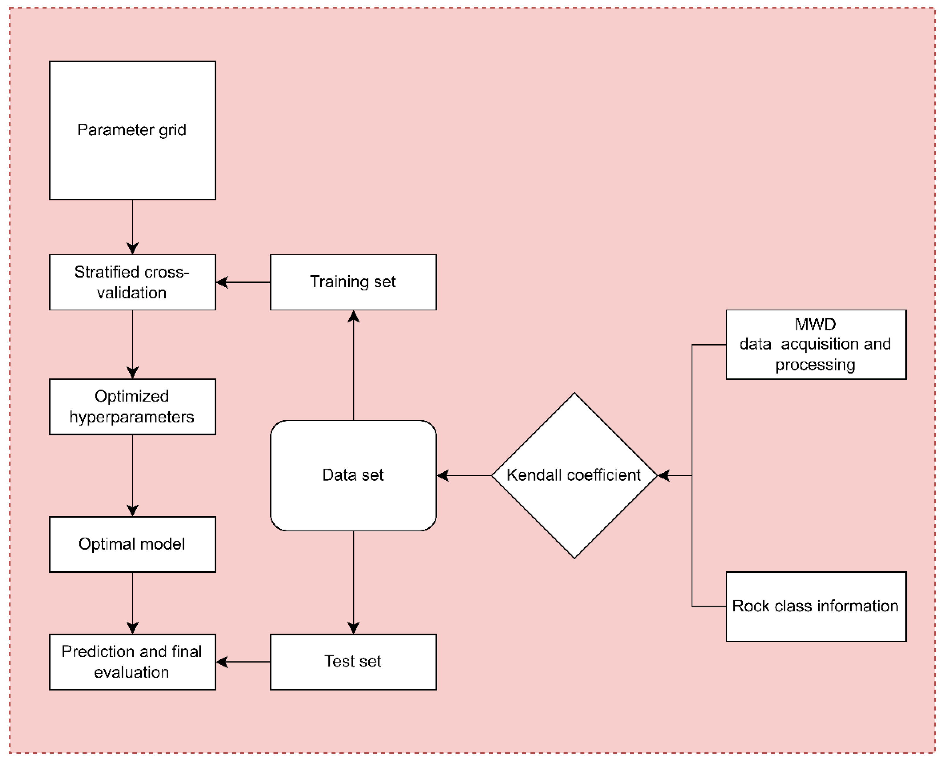
Figure 16 shows the workflow of the rock-mass classification prediction for each model. We selected the optimized hyperparameters using the grid-search method [36] to ensure that the resulting hyperparameters are the best possible. Accuracy was used as the evaluation metric to perform hyperparameter tuning based on the stratified 10-fold CV. The tuning results are shown in Table 6, with parameters not marked being the default values. The stratified 10-fold CV accuracies of the three methods are shown in Figure 17a; the mean accuracy is shown in Figure 17b, from which it can be seen that the model accuracies were BILSTM > MLP > SVM, indicating that the BILSTM model had the best ability to identify the surrounding rock classes.
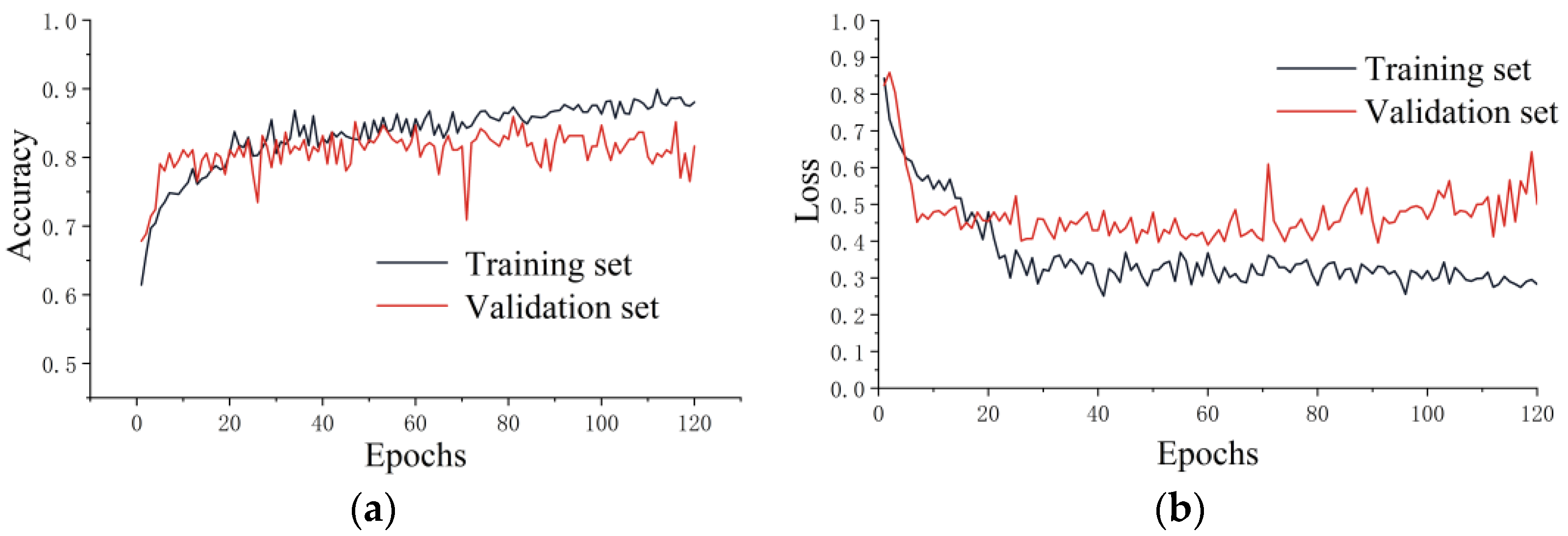
The model with the highest accuracy in the 10-fold model was used as the prediction model. Based on the results shown in Figure 17a, the BILSTM, MLP, and SVM selected the fold7, fold9, and fold3 models as rock-class prediction models for the test set. Figure 18 and Figure 19 illustrate the training processes for the prediction models of BILSTM and MLP, respectively. From the figure, it can be seen that the accuracy and loss curves of the BILSTM were stable, indicating that the BILSTM model proposed in this paper was reliable without overfitting; the curve of the MLP was not so stable and the loss curve of the validation set had an upward trend at the end, and there were overfitting phenomena. The actual rock classes for the test set and the prediction results of the three methods are shown in Figure 20; scatter plots are shown in Figure 21.
Figure 21 shows that the BILSTM and SVM models performed better regarding the prediction of class III surrounding rocks, involving fewer errors, with no obvious differences evident in the figure, while the MLP model performed in general. For the prediction of class IV surrounding rocks, the prediction accuracy of the three methods decreased, with the final performances being BILSTM > MLP > SVM, and the SVM model having more error points. For the prediction of class V surrounding rocks, the BILSTM model was the best, and the other two models had similar prediction results. Figure 20 and Figure 21 show that the BILSTM model proposed in this study outperforms the other two methods.
The performance and prediction results of each model were quantitatively evaluated and compared using the evaluation metrics in Section 3.2. The results of each evaluation metric are shown in Table 7, where the following can be seen: (1) All metrics of the BILSTM model were higher than those of the other two models; hence, the BILSTM model exhibited better prediction ability, with the values of each metric being Accuracy overall   = 0.900,   Precision overall = 0.904 ,   Recall overall = 0.898 , and F 1 overall = 0.900 . (2) For the prediction of a certain class of surrounding rock, the BILSTM model exhibited excellent performance. Taking class V surrounding rocks as an example, we considered the precision, recall, and F1 metrics together. Regarding precision, the BILSTM model had 0.889, while the MLP and SVM models had 1.000; regarding recall, the BILSTM model had 0.889, while the MLP and SVM models had 0.722 and 0.611, respectively; regarding the F1 value, the BILSTM model had 0.889, while the MLP and SVM models had 0.839 and 0.759, respectively. Combining the results of the three metrics, even though the precision of the BILSTM model was lower than those of the MLP and SVM models, it can still be concluded that the prediction ability of the BILSTM model for class V surrounding rocks was better than those of the MLP and SVM models.
The confusion matrices for the three methods are shown in Figure 22, and the micro- and macro-average ROCs and their corresponding AUC values are shown in Figure 23 and Table 8, respectively, where the following can be seen: (1) The macro- and micro-average AUC values of the BILSTM model were 0.9831 and 0.9814, respectively, the macro- and micro-average AUC values of the MLP model were 0.9209 and 0.9305, respectively, and the macro- and micro-average AUC values of the SVM model were 0.9212 and 0.9176, respectively. The BILSTM model exhibited the best performance. (2) Comparing the ROCs of the BILSTM, MLP, and SVM models also showed that the BILSTM model had the best prediction performance. (3) The difference between the macro- and micro-average AUC values can reflect the model’s ability to predict unbalanced datasets; it can be seen that the BILSTM model had the smallest difference, indicating that it can predict unbalanced datasets better than the MLP and SVM models.
Overfitting reflects the poor generalization ability of the model, i.e., the model has good performance in the training set, but poor performance in the test set. To assess the overfitting, the BILSTM, MLP, and SVM models were used to predict the training and test sets. Table 9 presents the results. The performance was evaluated based on accuracy, and the differences between the training-set and test-set accuracies were used to evaluate the generalization performance of the model. Table 9 shows the following: (1) The BILSTM model had the highest accuracy values in both the training and test sets, thereby proving its high performance. (2) The difference values of the BILSTM, MLP, and SVM models were 0.054, 0.116, and 0.094, respectively. The value of the BILSTM model was the lowest, indicating that it has a good generalization performance, followed by that of the SVM model, while the MLP model exhibited the worst generalization. Although the MLP and SVM models performed well on the training set, they performed poorly on the test set and suffered from overfitting.
The BILSTM deep neural network model proposed in this paper can handle unbalanced datasets well and performs well while predicting the surrounding rock classes. Applying this model in practical engineering can provide for the accurate identification of the surrounding rock classes in front of the tunnel face and serve as a basis for dynamically designing tunnels.

5. Conclusions

We proposed a novel deep neural network model for rock-mass classification based on depth-sequence MWD data, which can extract information related to the surrounding rock classes in both the forward and reverse directions, thereby improving the accuracy of the surrounding-rock classification prediction. In this model, we selected key parameters through Kendall coefficients and the deep neural network model uses BILSTM as the core, supplemented by two fully connected layers to integrate class-distinct local information, and the ‘window selector’, ‘Voter’, and other modules designed in the network to cooperate with one another and improve the generalization ability and prediction performance of the model. In addition, stratified K-fold cross-validation was used for model optimization to avoid overfitting in small datasets. BN was used to solve the ICS problem and improve the model prediction performance and multiple evaluation metrics were used to provide a comprehensive evaluation of the model’s performance from various perspectives.
After the structural design was completed, we created a dataset based on the advanced drilling data from a highway tunnel in Yunnan Province, China, and the BILSTM-based deep neural network was used to predict the class of the surrounding rock. The model was compared with the MLP and SVM models based on the same dataset, and the performances of the three models were evaluated from different aspects through multiple evaluation metrics. We confirmed that the proposed BILSTM-based deep neural network has the best prediction performance. Specific conclusions are as follows:
  • Compared with the MLP and SVM models, the BILSTM model has the best prediction ability, with the results of each metric being Accuracy 10 CV = 0.896 , Accuracy overall = 0.900 , Precision overall = 0.904 , Recall overall = 0.898 , F 1 overall = 0.900 , Micro _ average _ Auc = 0.9814 , Macro _ average _ Auc = 0.9831 , i.e., all significantly higher than those of the MLP and SVM models.
  • The accuracies of the BILSTM model were 0.954 and 0.900 in the training and test sets, respectively, with the difference being 0.054. The difference of the BILSTM model was the smallest compared with those of the MLP and SVM models, meaning that it had the best generalization performance. The other two methods performed well in the training set but poorly in the test set, with poor generalization and overfitting.
  • The average 10-fold CV accuracy of the BILSTM model was slightly lower than that in the test set. This is because the data in the training, validation, and test sets all came from the same tunnel, with the dataset being homogeneous. The results for the validation set were that the average of the 10-fold CV accuracy and the generalization of the BILSTM model were high, while the results for the test set were only single results; it is reasonable that they were slightly higher than the average 10-fold CV accuracy.
  • For class III surrounding rocks, with a large number of samples, all three methods exhibited high accuracies; for classes IV and V, with a small number of samples, the accuracies of all three methods decreased, but that of the BILSTM model was significantly higher than those of the other two methods, indicating that it has the best processing capability for unbalanced datasets.

Author Contributions

X.C.: Investigation, Data curation, Formal analysis, Methodology, Visualization, Software, Writing—original draft. H.T.: Investigation, Data curation, Supervision, Funding acquisition, Project administration. Z.W.: Investigation, Data curation, Writing—review and editing, Supervision, Funding acquisition, Conceptualization. D.L.: Data curation, Validation. Y.X.: Writing—review and editing, Validation. All authors have read and agreed to the published version of the manuscript.

Funding

This research was funded by Traffic Science and Technology Project of Yunnan Province, China. Grant No. [2020]-74 and Grant No. [2020]-98.

Data Availability Statement

The data presented in this study are available on request from the corresponding author. The data are not publicly available due to privacy.

Acknowledgments

We also express our heartfelt thanks to the editors and reviewers for providing very valuable suggestions to improve the quality of our manuscript.

Conflicts of Interest

The authors declared that they do not have any conflict of interest to disclose.

References

  1. Xu, X.J.; Zhang, P.L.; Guo, X.; Liu, B.; Chen, L.; Zhang, Q.S.; Nie, L.C.; Zhang, Y. A case study of seismic forward prospecting based on the tunnel seismic while drilling and active seismic methods. Bull. Eng. Geol. Environ. 2021, 80, 3553–3567. [Google Scholar] [CrossRef]
  2. Zhang, D.; Sun, Z.; Fang, Q. Scientific problems and research proposals for Sichuan–Tibet railway tunnel construction. Undergr. Space 2022, 7, 419–439. [Google Scholar] [CrossRef]
  3. Koopialipoor, M.; Tootoonchi, H.; Jahed Armaghani, D.; Tonnizam Mohamad, E.; Hedayat, A. Application of deep neural networks in predicting the penetration rate of tunnel boring machines. Bull. Eng. Geol. Environ. 2019, 78, 6347–6360. [Google Scholar] [CrossRef]
  4. Kitchah, F.; Benmebarek, S.; Djabri, M. Numerical assessment of tunnel collapse: A case study of a tunnel at the East–West Algerian highway. Bull. Eng. Geol. Environ. 2021, 80, 6161–6176. [Google Scholar] [CrossRef]
  5. Ren, Q.; Xu, L.; Zhu, A.; Shan, M.; Zhang, L.; Gu, J.; Shen, L. Comprehensive safety evaluation method of surrounding rock during underground cavern construction. Undergr. Space 2021, 6, 46–61. [Google Scholar] [CrossRef]
  6. Hassanpour, J.; Rostami, J.; Khamehchiyan, M.; Bruland, A.; Tavakoli, H.R. TBM performance analysis in pyroclastic rocks: A case history of Karaj water conveyance tunnel. Rock Mech. Rock Eng. 2010, 43, 427–445. [Google Scholar] [CrossRef]
  7. Li, S.C.; Liu, B.; Xu, X.J.; Nie, L.C.; Liu, Z.Y.; Song, J.; Sun, H.F.; Chen, L.; Fan, K. An overview of ahead geological prospecting in tunneling. Tunn. Undergr. Space Technol. 2017, 63, 69–94. [Google Scholar] [CrossRef]
  8. Panthi, K.K.; Nilsen, B. Uncertainty analysis of tunnel squeezing for two tunnel cases from Nepal Himalaya. Int. J. Rock Mech. Min. 2007, 44, 67–76. [Google Scholar] [CrossRef]
  9. Somerton, W.H. A laboratory study of rock breakage by rotary drilling. Trans. Aime 1959, 216, 92–97. [Google Scholar] [CrossRef]
  10. Hamelin, J.P.; Levallois, J.; Pfister, P. Drilling parameters recording: New developments. In Bulletin of the International Association of Engineering Geology-Bulletin de l’Association Internationale de Géologie de l’Ingénieur; Springer: Berlin/Heidelberg, Germany, 1982; Volume 26, pp. 83–88. [Google Scholar]
  11. Schunnesson, H. RQD predictions based on drill performance parameters. Tunn. Undergr. Space Technol. 1996, 11, 345–351. [Google Scholar] [CrossRef]
  12. Yue, Z.Q.; Lee, C.F.; Law, K.T.; Tham, L.G. Automatic monitoring of rotary-percussive drilling for ground characterization—Illustrated by a case example in Hong Kong. Int. J. Rock Mech. Min. 2004, 41, 573–612. [Google Scholar] [CrossRef]
  13. Wang, Q.; Gao, H.K.; Yu, H.C.; Jiang, B.; Liu, B.H. Method for measuring rock mass characteristics and evaluating the grouting-reinforced effect based on digital drilling. Rock Mech. Rock Eng. 2019, 52, 841–851. [Google Scholar] [CrossRef]
  14. Liang, D.C.; Tang, H.; Wu, Z.J.; Zhang, Y.H.; Fang, Y.W. Stratum identification based on multiple drilling parameters and probability classification. Rock Soil Mech. 2022, 43, 1123–1134. [Google Scholar] [CrossRef]
  15. Wang, Q.; Gao, S.; Li, S.; He, M.; Gao, H.; Jiang, B.; Jiang, Y. Upper bound analytic mechanics model for rock cutting and its application in field testing. Tunn. Undergr. Space Technol. 2018, 73, 287–294. [Google Scholar] [CrossRef]
  16. Bo, Y.; Liu, Q.; Huang, X.; Pan, Y. Real-time hard-rock tunnel prediction model for rock mass classification using CatBoost integrated with Sequential Model-Based Optimization. Tunn. Undergr. Space Technol. 2022, 124, 104448. [Google Scholar] [CrossRef]
  17. Lu, J.; Guo, W.; Liu, J.; Zhao, R.; Ding, Y.; Shi, S. An Intelligent Advanced Classification Method for Tunnel-Surrounding Rock Mass Based on the Particle Swarm Optimization Least Squares Support Vector Machine. Appl. Sci. 2023, 13, 2068. [Google Scholar] [CrossRef]
  18. Benemaran, R.S.; Esmaeili-Falak, M.; Javadi, A. Predicting resilient modulus of flexible pavement foundation using extreme gradient boosting based optimised models. Int. J. Pavement Eng. 2022, 1–20. [Google Scholar] [CrossRef]
  19. Esmaeili-Falak, M.; Benemaran, R.S. Ensemble deep learning-based models to predict the resilient modulus of modified base materials subjected to wet-dry cycles. Geomech. Eng. 2023, 32, 583–600. [Google Scholar]
  20. LaBelle, D. Lithological Classification by Drilling. Thesis Proposal, Robotics Institute, Carnegie Mellon University, Pittsburgh, PA, USA, 2001. [Google Scholar]
  21. Gao, H.K.; Wang, Q.; Jiang, B.; Zhang, P.; Jiang, Z.H.; Wang, Y. Relationship between rock uniaxial compressive strength and digital core drilling parameters and its forecast method. Int. J. Coal Sci. Technol. 2021, 8, 605–613. [Google Scholar] [CrossRef]
  22. Ameur-Zaimeche, O.; Kechiched, R.; Heddam, S.; Wood, D.A. Real-time porosity prediction using gas-while-drilling data and machine learning with reservoir associated gas: Case study for Hassi Messaoud field, Algeria. Mar. Pet. Geol. 2022, 140, 105631. [Google Scholar] [CrossRef]
  23. Kadkhodaie-Ilkhchi, A.; Monteiro, S.T.; Ramos, F.; Hatherly, P. Rock recognition from MWD data: A comparative study of boosting, neural networks, and fuzzy logic. IEEE Geosci. Remote Sens. Lett. 2010, 7, 680–684. [Google Scholar] [CrossRef]
  24. Fang, Y.W.; Wu, Z.J.; Sheng, Q.; Tang, H.; Liang, D.C. Tunnel geology prediction using a neural network based on instrumented drilling test. Appl. Sci. 2020, 11, 217. [Google Scholar] [CrossRef]
  25. Klyuchnikov, N.; Zaytsev, A.; Gruzdev, A.; Ovchinnikov, G.; Antipova, K.; Ismailova, L.; Koroteev, D. Data-driven model for the identification of the rock type at a drilling bit. J. Petrol. Sci. Eng. 2019, 178, 506–516. [Google Scholar] [CrossRef]
  26. Romanenkova, E.; Zaytsev, A.; Klyuchnikov, N.; Gruzdev, A.; Antipova, K.; Ismailova, L.; Koroteev, D. Real-time data-driven detection of the rock-type alteration during a directional drilling. IEEE Geosci. Remote Sens. Lett. 2019, 17, 1861–1865. [Google Scholar] [CrossRef]
  27. Gupta, I.; Tran, N.; Devegowda, D.; Jayaram, V.; Rai, C.; Sondergeld, C.; Karami, H. Looking ahead of the bit using surface drilling and petrophysical data: Machine-learning-based real-time geosteering in Volve field. SPE J. 2020, 25, 990–1006. [Google Scholar] [CrossRef]
  28. Kendall, M.G. A new measure of rank correlation. Biometrika 1938, 30, 81–93. [Google Scholar] [CrossRef]
  29. Matwin, S.; Mielniczuk, J. Challenges in Computational Statistics and Data Mining; Springer: Cham, Switzerland, 2016. [Google Scholar]
  30. Xiao, H.H.; Yang, W.K.; Hu, J.; Zhang, Y.P.; Jing, L.J.; Chen, Z.Y. Significance and methodology: Preprocessing the big data for machine learning on TBM performance. Undergr. Space 2022, 7, 680–701. [Google Scholar] [CrossRef]
  31. Hochreiter, S.; Schmidhuber, J. Long short-term memory. Neural Comput. 1997, 9, 1735–1780. [Google Scholar] [CrossRef]
  32. Ioffe, S.; Szegedy, C. Batch normalization: Accelerating deep network training by reducing internal covariate shift. In Proceedings of the International Conference on Machine Learning, Lille, France, 6–11 July 2015; pp. 448–456. [Google Scholar]
  33. Di Martino, M.; Fernández, A.; Iturralde, P.; Lecumberry, F. Novel classifier scheme for imbalanced problems. Pattern Recogn. Lett. 2013, 34, 1146–1151. [Google Scholar] [CrossRef]
  34. Industrial Standard of the People’s Republic of China. Specifications for Design of Highway Tunnels Section 1 Civil Engineering: JTG 3370. 1-2018; China Communications Press: Beijing, China, 2018; ISBN 978-7-114-14639-8. [Google Scholar]
  35. TensorFlow Developers. TensorFlow (v2.12.0). Zenodo. 2023. Available online: https://doi.org/10.5281/zenodo.7764425 (accessed on 23 March 2023).
  36. Yan, T.; Shen, S.L.; Zhou, A.; Chen, X. Prediction of geological characteristics from shield operational parameters by integrating grid search and K-fold cross validation into stacking classification algorithm. J. Rock Mech. Geotech. 2022, 14, 1292–1303. [Google Scholar] [CrossRef]
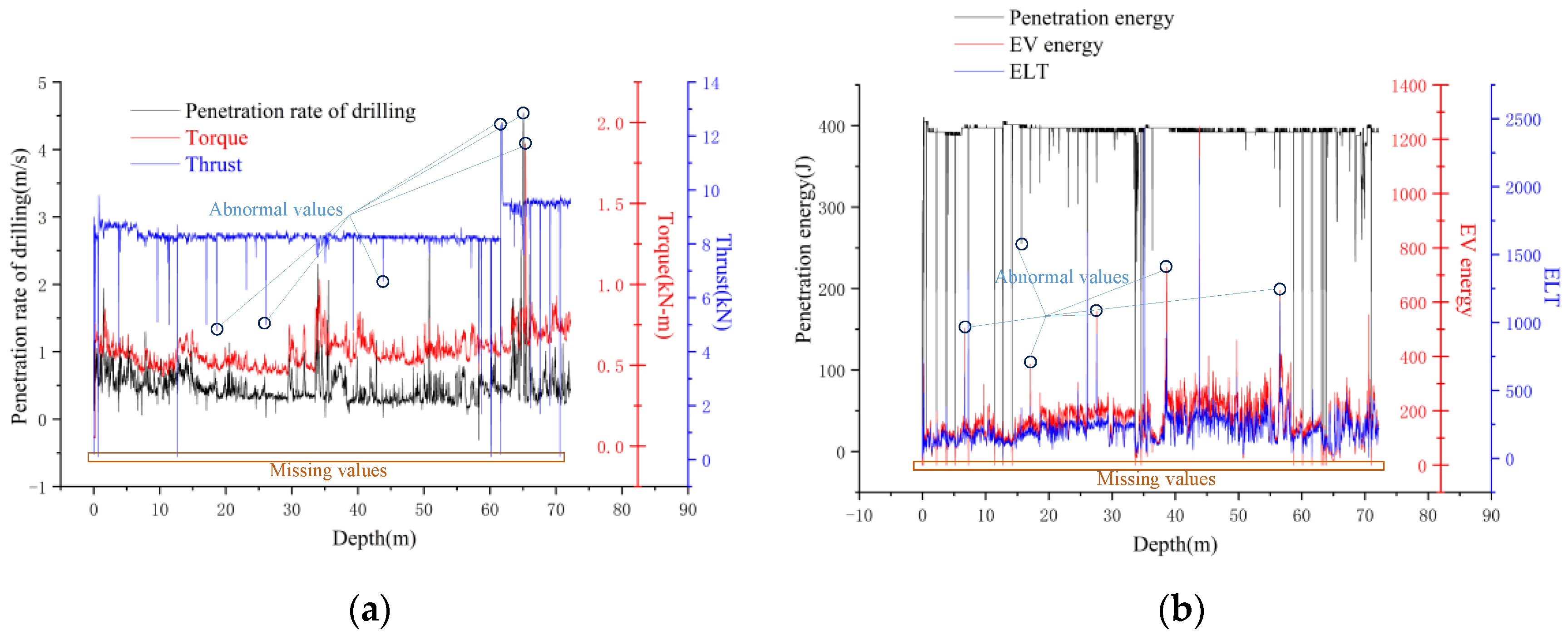
Figure 1. Typical variation of some drilling parameters. (a) Penetration rate of drilling, Torque, and Thrust variation and (b) Penetration energy, EV energy, and ELT variation.
Applsci 13 06050 g001
Figure 2. Workflow of the deep neural network combing k-fold cross-validation.
Applsci 13 06050 g002
Figure 3. Long short-term memory (LSTM) structure.
Applsci 13 06050 g003
Figure 4. Bidirectional long short-term memory (BILSTM) structure.
Applsci 13 06050 g004
Figure 5. Structure sketch of the fully connected (FC) layer; (a) The first two fully connected layers; (b) The last fully connected layer.
Applsci 13 06050 g005
Figure 6. Window selector.
Applsci 13 06050 g006
Figure 7. Structure of the deep neural network.
Applsci 13 06050 g007
Figure 8. Confusion matrix.
Applsci 13 06050 g008
Figure 9. Location of the Tunnel.
Applsci 13 06050 g009
Figure 10. Geological profile of the tunnel route.
Applsci 13 06050 g010
Figure 11. The tunnel collapsed.
Applsci 13 06050 g011
Figure 12. The accuracy of different key parameters.
Applsci 13 06050 g012
Figure 13. Rock class distributions. (a) Dataset, (b) training set, and (c) test set.
Applsci 13 06050 g013
Figure 14. Frequency distribution of the training set.
Applsci 13 06050 g014
Figure 15. Frequency distribution of the test set.
Applsci 13 06050 g015
Figure 16. Workflow of the rock-mass classification prediction for each model.
Applsci 13 06050 g016
Figure 17. Cross-validation accuracies. (a) Stratified 10-fold CV accuracies and (b) Stratified 10-fold CV mean accuracies.
Applsci 13 06050 g017
Figure 18. Accuracy and Loss curves on training set and validation set of BILSTM-based deep neural network. (a) Accuracy curve and (b) Loss curve.
Applsci 13 06050 g018
Figure 19. Accuracy and Loss curves on training set and validation set of MLP neural network. (a) Accuracy curve and (b) Loss curve.
Applsci 13 06050 g019
Figure 20. Actual classes and predicted results.
Applsci 13 06050 g020
Figure 21. Scatter plot of the actual class predicted results. (a) BILSTM, (b) MLP, and (c) SVM.
Applsci 13 06050 g021
Figure 22. Confusion matrices: (a) BILSTM, (b) MLP, and (c) SVM.
Applsci 13 06050 g022
Figure 23. Macro–micro average ROCs: (a) BILSTM, (b) MLP, and (c) SVM.
Applsci 13 06050 g023
Table 1. Major drilling parameters.
Drilling ParameterUnitDrilling ParameterUnit
DepthmWater supply pressureMPa
TorquekN-mWater supply rateL/min
Rotation SpeedrpmDrainage pressureMPa
Percussive forcekNDrainage rateL/min
Beat per minutebpmEVJ/m3
ThrustkNELT-
Table 2. The p-value approach.
p-ValueCoincidence ProbabilityNull HypothesisStatistical Significance
p > 0.05Coincidence probability greater than 5%Cannot refuseNo significant difference
p ≤ 0.05Coincidence probability less than 5%RefuseSignificant difference
p ≤ 0.01Coincidence probability less than 1%RefuseVery significant difference
Table 3. Sensitivity analysis results.
Penetration Rate of DrillingTorqueRotation SpeedThrustPenetration
Energy
Beat Per MinuteWater Supply RateWater Supply PressureEVELTRock Class
Penetration Rate of Drilling1.000 0.268 −0.008 −0.255 0.028 0.028 0.042 −0.025 −0.916 −0.948 −0.406
Torque0.268 1.000 0.070 −0.074 −0.134 −0.134 −0.108 0.295 −0.289 −0.253 −0.242
Rotation Speed−0.008 0.070 1.000 −0.013 0.059 0.059 −0.103 0.081 0.012 0.012 −0.002
Thrust−0.255 −0.074 −0.013 1.000 0.096 0.096 −0.034 0.019 0.274 0.311 0.167
Penetration Energy0.028 −0.134 0.059 0.096 1.000 1.000 0.046 −0.131 0.074 −0.014 0.136
Beat Per Minute0.028 −0.134 0.059 0.096 1.000 1.000 0.046 −0.131 0.074 −0.014 0.136
Water Supply Rate0.042 −0.108 −0.103 −0.034 0.046 0.046 1.000 −0.096 −0.046 −0.043 −0.001
Water Supply Pressure−0.025 0.295 0.081 0.019 −0.131 −0.131 −0.096 1.000 0.025 0.034 −0.083
EV−0.916 −0.289 0.012 0.274 0.074 0.074 −0.046 0.025 1.000 0.900 0.433
ELT−0.948 −0.253 0.012 0.311 −0.014 −0.014 −0.043 0.034 0.900 1.000 0.403
Rock Class−0.406 −0.242 −0.002 0.167 0.136 0.136 −0.001 −0.083 0.433 0.403 1.000
Table 4. Statistics of the key drilling parameters in the training set.
Key Drilling ParametersUnitMaxMinMeanMedian
Penetration rate of drillingm/min4.960.000.420.31
TorquekN-m1.870.020.680.65
ThrustkN36.300.008.938.80
Penetration energyJ423.000.00376.05392.00
EV\6448.000.00239.98201.00
Table 5. Statistics of the key drilling parameters in the test set.
Key Drilling ParametersUnitMaxMinMeanMedian
Penetration rate of drillingm/min3.690.000.470.32
TorquekN-m1.720.050.650.62
ThrustkN21.000.008.798.60
Penetration energyJ410.000.00378.83388.00
EV\6448.000.00227.87198.00
Table 6. Optimization results of the hyperparameters of each model.
ModelOptimized Hyperparameters
BILSTMlearning_rate = 0.01; epoch = 120; drop_out = 0.3;
l2_regularization = 5 × 10⁻⁵; layer_1_units = 20;
layer_2_units = 20; LSTM_hidden_units = 32.
SVCC = 7; kernel = ‘rbf’; gamma = 47.
MLPlearning_rate = 0.01; epoch = 120; drop_out = 0.3;
l2_regularization = 5 × 10⁻⁵; hidden_layer_1_units = 20;
hidden_layer_2_units = 20.
Table 7. Results of the evaluation metrics.
MethodRock Mass ClassAccuracyPrecisionRecallF1Support
BILSTMIII 0.883 0.964 0.922 55
IV 0.955 0.778 0.857 27
V 0.889 0.889 0.889 18
Overall0.900 0.904 0.898 0.900 100
MLPIII 0.821 0.836 0.828 55
IV 0.581 0.667 0.621 27
V 1.000 0.722 0.839 18
Overall0.770 0.789 0.774 0.770 100
SVMIII 0.711 0.982 0.825 55
IV 0.769 0.370 0.500 27
V 1.000 0.611 0.759 18
Overall0.750 0.778 0.725 0.750 100
Table 8. Macro–micro average AUC values.
MethodMacro_Average_AUCMicro_Average_AUCDifference
BILSTM0.98310.98140.0017
MLP0.92090.9305−0.0096
SVM0.92120.91760.0036
Note: Difference = Macro_average_AUC -Micro_average_AUC.
Table 9. Predicted results for the training and test sets.
MethodTraining-Set AccuracyTest-Set AccuracyDifference
BILSTM0.9540.900 0.054
MLP0.8860.770 0.116
SVM0.8440.750 0.094
Note: Difference = Training-set accuracy—Test-set accuracy.
Disclaimer/Publisher’s Note: The statements, opinions and data contained in all publications are solely those of the individual author(s) and contributor(s) and not of MDPI and/or the editor(s). MDPI and/or the editor(s) disclaim responsibility for any injury to people or property resulting from any ideas, methods, instructions or products referred to in the content.