Abstract
The tendon that is inserted into the duct is a crucial component of prestressed concrete (PSC) bridges and, when exposed to air, can quickly corrode, and cause structural collapse. It can interpret the signal measured by non-destructive testing (NDT) to determine the condition (normal or void) inside the duct. However, it requires the use of expensive NDT equipment such as ultrasonic waves or the hiring of experts. In this paper, we proposed an impact–echo (IE) method based on deep support vector data description (Deep SVDD) for economical void detection inside a duct. Because the pattern of IE changes for various reasons such as difference of specimen or bridge, supervised learning is not suitable. Deep SVDD is classified as normal and defective, which is a broad distribution as a hypersphere that encloses a multi-dimensional feature space for normal data represented by an autoencoder. Here, an autoencoder was developed based on the ELMo (embeddings from language model)-like structure to obtain an effective representation for IE. In the experiment, we evaluated the performance of the IE data measured in different specimens. Thus, our proposed model showed an accuracy of about 77.84% which is an improvement of up to about 47% compared to the supervised learning approach.
1. Introduction
A cost-effective civil engineering material that is frequently utilized in nuclear power plants, dams, and bridges is prestressed concrete (PSC) [1]. PSC ensures the stability of the structure by employing a tendon to provide pre-tension and post-tension to address the issue of concrete that is susceptible to tensile stress. The PSC bridge is a construction that makes the greatest use of the PSC technique (post-tension) and guarantees structural stability when developing a lengthy bridge [2]. A duct (also known as a sheath) is a tube that is used in the post-tensioning technique to apply tensile stress afterwards. To put it another way, when the duct has been installed, a tendon is put inside it to generate tensile tension, and then concrete is poured to fix it. As a result, tendons are essential to the security of buildings. The tendon, however, experiences defects such as rust when it is exposed to air, which is why it is placed within the duct before concrete is poured. A defect such as rust might result in an abrupt structural collapse [2].
However, the following two restrictions apply to the tendon. First, the duct’s inner diameter is quite small. Second, the duct is mounted in a curved construction. For this reason, even a small mistake might result in a void within the duct. Because of this, it is crucial to assess the duct’s inside condition, which calls for great precision.
A proposed technique for exploring the inside of concrete structures is non-destructive testing (NDT). It measures the signals produced by ultrasonic waves, radiation, magnetic fields, and the impact–echo (IE) method to explore the internal condition of the concrete structure [3,4,5,6,7,8]. However, this method requires the hiring of experts for complex and academic interpretation and it is a challenge to interpret accurately due to the complicated internal structure of the PSC bridge and the lack of suitable NDT. Another way is to use expensive NDT equipment such as ultrasonic wave-based equipment, but problems such as equipment size or budget still exist. For this reason, in most cases, it has been confirmed for safety by direct drilling based on experience. To interpret the voids that exist inside the ducts of PSC bridges, additional useful and economical methodologies are therefore required.
In the early studies, the IE method was widely used to identify voids in concrete structures [9,10,11]. It analyzes the frequency spectrum extracted by Fourier transform. However, because there is a strong likelihood that multiple peaks may occur as a reason for vibration or something similar, it has been challenging to correctly interpret this frequency spectrum by experts [12]. To address this issue, many studies try to use time-frequency analysis such as wavelet transform (WT), short-time Fourier transform (STFT), empirical mode decomposition (EMD), and Hilbert–Huang transform (HHT), a signal processing-based approach [12,13,14,15]. When [16] compared various time-frequency analyses, it was discovered that WT was the most useful for interpreting the IE method.
On the other hand, machine learning-based approaches concentrate on assessing the condition of specific concrete components or entire concrete structures. Most of studies have used image-based crack detection or structural health monitoring (SHM) [17,18]. Some studies have tried to detect defects that occur inside concrete structures. After applying WT to the IE data, [19] used the extreme learning machine (ELM) [20] approach to assess the overall condition of the concrete structure, and its good performance demonstrated the promise of machine learning. The authors of [21,22] used a convolutional neural network (CNN) [23] and long short-term memory (LSTM) [24] approach to assess the bridge deck’s internal defects and confirmed their potential. According to this trend, efforts have recently been made to provide a gold-standard measurement using the IE method [25].
Detecting voids that arise inside the ducts of PSC bridges is a particularly significant issue; however, it has only been investigated using a signal processing-based method, and machine learning is rarely applied. Therefore, by utilizing IE data and LSTM, supervised learning was attempted to detect defects inside ducts in previous studies [26,27,28]. Utilizing IE data and structural information (concrete thickness, depth of duct, distance between the measured point and impact point), [26] used LSTM to classify the duct’s voids. However, we determined that the structural information affects the scalability of the deep learning-based approach. Therefore, [27,28] developed an LSTM-based model that can use a frequency spectrum with IE data.
These experiments demonstrated good performance; however, a significant issue was found: the pattern of the IE data appears irregular. For example, the pattern of the IE data of the specimen used for training and the IE data of the new specimen or PSC bridge appear different. This phenomenon was found even for the new specimen, in the same conditions. In addition, if there are voids on the opposite side of the measurement point, another pattern appears, making it difficult to detect. Consequently, it is required to provide training data with a variety of patterns, but doing so is actually a challenging undertaking. As a result, the supervised learning models trained to the specimen’s IE data found only part of the voids in real-world PSC bridges. To minimize these issues, a deep learning approach that can flexibly utilize both the data used for training and the data measured elsewhere is required. In particular, cases where voids occur in industrial sites are extremely rare (i.e., class imbalance issue).
In this paper, we used deep support vector data description (Deep SVDD) [29] to solve the limitations of supervised learning due to the characteristics of the IE method. Basically, Deep SVDD, which is a semi-supervised learning approach, establishes a hypersphere around normal data, reduces the size of this boundary, and classifies all data outside the hypersphere as abnormal. In other words, Deep SVDD assumes that the distribution of normal and abnormal data is different. Due to these characteristics, we considered it suitable for solving the class imbalance issue and the limitation of the IE method that appears in irregular patterns (or distributions), whether they are normal or voids. At this time, Deep SVDD utilizes a pre-trained autoencoder that can represent the normal data and defect the data distribution differently for the inputs. So, it is important to design a suitable autoencoder structure that can represent the distribution of input data (normal data and void data) differently. Therefore, we developed the autoencoder based on an ELMo (embeddings from language model)-like LSTM architecture [30] because ELMo represents the context well. It trains in both the forward and backward directions, unlike bidirectional LSTM (Bi-LSTM). Then, Deep SVDD trains a minimized hypersphere surrounding the feature space (i.e., latent vector in autoencoder) for the IE data, which are normal data, and determines the IE data outside of this hypersphere as a void. For the experiment, we evaluated the performance of our proposed model using IE data collected from two different specimens and compared it with the supervised learning models which were developed in previous studies.
The format of this paper is as follows. Section 2 describes the IE data collected for the experiment as well as the issues we discovered with the IE data. Our proposed method is described in Section 3, and the experimental results are provided in Section 4. Finally, Section 5 concludes with a summary of our findings.
2. Impact–Echo Data
A PSC bridge provides compressive stress to the concrete in order to minimize the generation of tensile stress; it uses a method in which tensile stress is applied later using a duct. In this paper, we used the PSC specimens manufactured by the Korea Institute of Civil engineering and building Technology (KCIT, Goyang-si, Republic of Korea) (https://www.kict.re.kr; accessed on 2 March 2022) to verify our proposed method, which was manufactured based on the same structure and material as close as possible to the actual PSC bridges. One is a specimen manufactured with various thicknesses (Specimen−1), and the other is a specimen manufactured with the same thickness and vertical shape (Specimen−2). These specimens have both a void structure and a normal structure. Figure 1 is an illustration of a cross-sectional view of a PSC bridge’s internal structure.
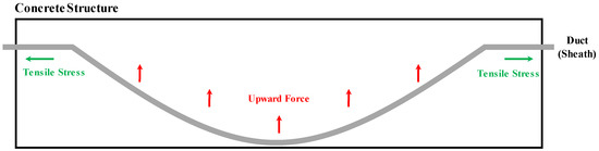
Figure 1.
Structure of PSC girder bridge.
The IE method is a method developed for the non-destructive testing (NDT) of concrete structures based on the principle of measuring the impact-generated stress waves that transmit an impact to the concrete surface and are reflected from the surface of different materials. In this paper, we consider that the principle of reflection from different materials along with the economic advantages of the IE method can include information on internal defects. The IE equipment which is manufactured by Olson Instruments Inc. (Wheat Ridge, CO, USA) (https://www.olsoninstruments.com; accessed on 22 February 2022) was used in this paper and the principles of the IE method are shown in Figure 2 and Figure 3. Additionally, Figure 4 shows the measured IE data samples in Specimen−1. In Figure 4, the IE data have a considerable amplitude during specific areas of the measurement time.
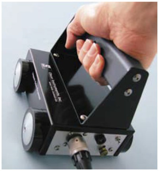
Figure 2.
IE equipment used in this paper.
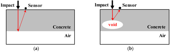
Figure 3.
(a) Basic principle of IE; (b) examples of IEs that may contain information of internal defect.
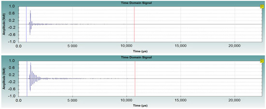
Figure 4.
Example of IE data in Specimen−1 (top: normal, bottom: defect).
However, there is one thing we need to consider when using the IE method: the pattern of IE data appears irregular. This phenomenon is affected not only when measuring different specimens or bridges, but also on the compressive strength and modulus of concrete. In concrete structures, the compressive strength and modulus of concrete change continuously over time [31]. The causes are climate changes, temperature variations, or other environmental factors [32,33]. For example, the constant stresses and vibrations caused by vehicles crossing a bridge have an impact on it. Climate change is particularly dangerous for concrete since it expands and contracts in response to temperature variations. As a result, concrete ages more quickly over time and structures lose strength from corrosion [33]. For this reason, it can lead to a difference in the pattern of IE even in the same conditions.
Therefore, we compared IE data measured in Specimen−1 and Specimen−2, as shown in Figure 5. Here, the IE data of Specimen−1 show a value measured at a different time from the IE data of Figure 4. Figure 5a,b are the normal data measured at Specimen−1 and Specimen−2, but it can be seen that the patterns of the IE data are different. Similarly, it can be seen that different patterns appear in Figure 5c,d, which are the void data. In particular, it can be confirmed that Figure 5a,c show different patterns compared to Figure 4. Finally, it is clear from Figure 4 and Figure 5 that most of the IE data have an amplitude in a specific area. Therefore, we chose this specific area and used its amplitude value as a training feature.
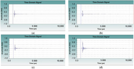
Figure 5.
IE data in different specimens show different patterns. (a) Normal IE data (Specimen−1); (b) normal IE data (Specimen−2); (c) void IE data (Specimen−1); (d) void IE data (Specimen−2).
3. Void Detection Based on Deep SVDD
In this section, we describe the architecture of the model that we propose for detecting voids occurring inside the duct. First, we standardized the raw IE data. Next, the autoencoder representing a feature space of the IE data was then used as a feature space in Deep SVDD. At this time, the autoencoder uses the ELMo-like LSTM architecture. Last but not least, Deep SVDD determines the minimum boundary of the hypersphere enclosing the feature space of the IE data which are represented as normal by the encoder of the autoencoder, and it deems the IE data which are outside this hypersphere to be defective. Figure 6 shows the overall flow of our proposed model. Next, each component is detailed in further depth.
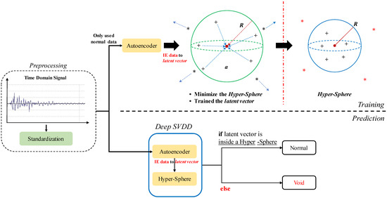
Figure 6.
The overall flow of our proposed model for void detection inside duct in PSC bridge.
3.1. Standardization
When comparing data from different normal distributions or carrying out statistical estimates for a particular normal distribution, standardization is used. It transforms the data mean and standard deviation to be 0 and 1, respectively. The standardization that we applied to the data is shown in Equation (1).
where is the value for each time-step of IE data, is the mean, and is the standard deviation.
3.2. Deep Support Vector Data Description
Support vector data description (SVDD) [34] uses a support vector machine (SVM) [35]-like kernel function to represent the feature space of the input. The hypersphere’s minimized boundary, which may identify the classes from the distribution of this feature space, is then determined. Therefore, SVDD is mapped so that normal data in the feature space are closer to the center point of the sphere, and defect data are further away by adding a penalty. Equation (2) describes the SVDD’s objective function.
where is the penalty imposed on the defect data, is the sphere’s radius, is the sphere’s center, and is the penalty constant. The fact that the data are mapped to the feature space by the kernel function (), and that the distance of the data from the sphere’s center must be located inside the area, is also can be verified by Equation (4) determines whether the data are normal or defects using the values of , , and obtained using this objective function. The input data are calculated to be positive if they are normal when inside the sphere, and negative if they are abnormal when outside the sphere.
In contrast, Deep SVDD [29] replaced the kernel function with an autoencoder which is the deep learning approach. In other words, the input’s feature space, or latent vector, is represented by the autoencoder. To distinguish between the feature spaces of normal and defective data provided by the autoencoder, Deep SVDD determines the minimum boundary of the hypersphere as follows: Deep SVDD trains data to be gathered more densely to the center point inside the hypersphere with a radius of . On the other hand, data outside of the hypersphere train to move further from the center point of the hypersphere, and Deep SVDD classifies data outside of the hypersphere as abnormal. Therefore, Deep SVDD determines the minimized boundary of the hypersphere that can distinguish the feature space of normal and defective data represented by the autoencoder as shown in Figure 7. Equation (4) is the object function that determines the hypersphere’s minimized boundary.
where is the hypersphere’s center and is the feature space that the autoencoder transformed from the input data. The left term calculates to minimize the distance between the feature space and , the hypersphere’s center. The right term is a weight decay regularizer, which prevents a particular weight from increasing excessively and trains it through optimization to map a normal data feature space close to . This allows Deep SVDD to define the anomaly score for input’s feature space as in Equation (5).
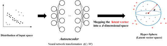
Figure 7.
Basic process of Deep SVDD.
To produce a feature space that suitably represents IE data, the autoencoder developed an ELMo-like structure, which will be covered in more detail in Section 3.3.
3.3. Autoencoder Based on ELMo
An autoencoder [36] is a deep learning approach that copies an input to an output, and consists of an encoder and a decoder. The encoder uses the input to train a latent vector, which is an encoded representation. Using a latent vector that the encoder represents, the decoder is trained to generate an output that is equivalent to the input. As compressed information about the input, the latent vector is the core of the autoencoder and must be designed in a way that can properly represent it.
ELMo (embeddings from language models) [30], a word-embedding method based on pretrained language models, was introduced in 2018. ELMo is a contextualized word embedding that reflects the fact that even the same vocabulary can have different meanings in different contexts. For this, ELMo used the LSTM, which achieved good performance in time series data. The LSTM comprises LSTM cells that are trained in a time order and have three gates (input gate, forget gate, output gate) equal to the length of the time series data. Information from the previous time step can be transferred to the current time step as the cell state () in the LSTM cell calculated by the out puts of the input gate () and forget gate (). Equations (6)–(11) describe how the LSTM cell is calculated.
While uses the hyperbolic tangent function to generate new candidate values from the input, uses the sigmoid function to determine which values in the input to update. The two outputs are used to produce a value that will update the cell state. determines how much information from is eliminated. To determine what information in should transfer, calculates the input as a sigmoid function. These outputs enable the LSTM cell to calculate , which represents the current information that will be transferred to the following time step. However, it does not include contextual information, so Bi-LSTMs that train forward and backward information are mainly used. Instead of a typical Bi-LSTM, ELMo uses a structure that trains word vectors represented in a pre-trained language model in the forward and backward directions, respectively. Figure 8 shows the difference between Bi-LSTM and ELMo.
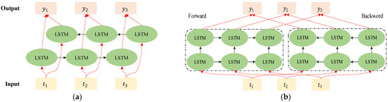
Figure 8.
(a) Example of Bi-LSTM’s structure; (b) example of ELMo’s structure.
Signals arise in the sequence of time. When performing an anomaly detection task, signals are evaluated in the forward direction to identify when a defect occurs. Environmental factors such as the characteristics of concrete structures and the geometry of irregular defects along with the utilization of impact-generated stress waves due to impact make IE different from other domain signals. For this process, we developed an autoencoder that, like ELMo, trains the forward and backward directions separately.
LSTM layers in the encoder train in the forward and backward directions, respectively. The output of each LSTM layer is transferred to the LSTM layer that trains in the same direction. The second LSTM layer’s outputs are all concatenated and used as latent vectors. By reversing the encoder, the decoder trains to provide an output that is equal to the input. In Deep SVDD, the feature space was represented using only the encoder structure of the autoencoder. The feature space represented by the encoder of the autoencoder is as shown in Equation (12).
where is a feature space which is latent vector in autoencoder. The encoder’s forward and backward LSTM outputs are denoted by the and , respectively. In Deep SVDD, the dimension of feature space is once more readjusted to utilize the feature space that was obtained in this way. The structure of such an autoencoder is shown in Figure 9.
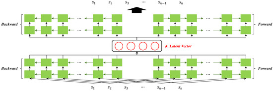
Figure 9.
Architecture of the autoencoder used in Deep SVDD.
4. Results and Discussion
In this paper, we collected IE data from two different structures (Specimen−1 and Specimen−2) as described in Section 2. In Specimen−1 and Specimen−2, this data collection amounted to 8000 and 11,231, respectively. In addition, we analyzed all the amplitude values for the data which occurred and chose a range from 880 to 2640 as the training feature. Table 1 contains detailed information on the IE dataset that we used.

Table 1.
Information of the IE data used as input features and the quantity collected in two specimens.
In the experiment, we determined the optimal parameters of the proposed model using the grid search method. We examined the dimension of feature space (i.e., hidden node) and loss function in Deep SVDD, as well as output sizes of the first and second LSTM layer in the encoder structure of the autoencoder. The decoder structure of the autoencoder is the reverse of the encoder structure of the autoencoder. First, we determined optimal parameters about the encoder and decoder structure of the autoencoder. As a result, we chose the optimal parameters for the output sizes of the first and second LSTM layers in the encoder structure to be 8 and 4, respectively. So, output sizes of the first and second LSTM layers in the decoder structure are 4 and 8, respectively. Second, the dimension of the feature space was readjusted in Deep SVDD is 32 and the dimension of the feature space represented in the encoder of the autoencoder is 320. Finally, a hard margin was used in Deep SVDD’s loss function. Table 2 shows them in detail. Finally, we used an early stopping method that stopped training when the loss of the validation data rose three times in a row to prevent overfitting.
Table 2.
Optimal parameters in our proposed model.
We carried out the following two evaluations in the experiment and compared the classification accuracy (Acc) for the normal and void data: (1) Examine the supervised learning model’s performance with IE data collected in the same environment. It performs training and evaluation using just Specimen−2 data divided in an 8:1:1 (train:validation:test) ratio. (2) With IE data collected in different environments, compare the performance of the supervised learning model [26,27,28] with our proposed models. It performs an evaluation using the IE data in Specimen−2 and trains using the IE data in Specimen−1. The two experiments support the issue we identified and demonstrate the superiority of the model we proposed for addressing it.
In the first experiment (using the IEs collected in the same specimen), we trained and evaluated the performance of the supervised learning model developed in the previous studies [26,27,28]. The results are shown in Table 3. As shown in Table 3, the supervised learning model in this instance had an extremely high accuracy. The effectiveness of supervised learning models in detecting defects in IE data with the same distribution may therefore be proven. However, the issue we discovered makes the use of supervised learning models challenging. So, we compared the performance using the IE data collected in different specimens in order to demonstrate that our proposed model could address this issue.
Table 3.
Evaluation of data collected in the same environment by supervised learning models.
As shown in Table 4, supervised learning models did not correctly distinguish between the normal and defective IEs collected in different specimens. Some models also showed a tendency to overfit. On the other hand, our proposed model showed an accuracy of about 77.84%. As well, it showed an average accuracy improvement of about 25% (up to around 47%) compared to the supervised learning model. In order to map the autoencoder’s feature space near to the center of the hypersphere, Deep SVDD trains the optimum (minimized) boundary surrounding the feature space of the normal data and determines it. At this time, the feature space of the normal data are also trained to be represented so that it nears the center of the hypersphere. We believe that by utilizing these Deep SVDD characteristics, normal data and void data in IE can be effectively distinguished in situations with different patterns compared to the supervised learning model.
Table 4.
Evaluation of data collected in different environments by supervised learning models and our proposed model.
5. Conclusions
In this paper, we used IE and Deep SVDD which is semi-supervised learning for detecting voids inside the ducts of PSC bridges and tried to address the following issues. We verified that the patterns of IE data measured in different specimens or PSC bridges differed. Here, we developed an autoencoder with an ELMo-like LSTM architecture to represent the feature space of the IE data well to effectively use Deep SVDD. To demonstrate the reliability of our proposed method, we compared the performance with supervised learning models. In the first experiment, we evaluated how well the supervised learning model performed using data measured in the same specimen, and it showed good performance. Next, we compared the performance of our proposed model with that of the supervised learning model on trained data and tested data in different specimens. The experiment revealed that our proposed model performed better on average than the supervised learning model by around 25.6% (up to about 47%), with an accuracy of about 77.84%. Thus, we believe that the Deep SVDD-like semi-supervised learning can be effectively applied to real-world anomaly detection tasks. However, it is considered that the performance of our proposed model is insufficient to be used for actual industry purposes, and a process of confirming it with IE data measured from more diverse specimens and actual PSC bridges is considered necessary.
In the future, we will systematically study the unsupervised anomaly detection approach and autoencoder architecture to develop a void detection technique inside the duct of PSC bridges that is more effective and superior to what is now available. Furthermore, we will find a way to collect IE data from real PSC bridges.
Author Contributions
Conceptualization, Y.-S.K. and H.C.; methodology, B.-D.O.; validation, C.-Y.P., H.C. and W.-J.C.; formal analysis, C.-Y.P., W.-J.C. and B.-D.O.; data curation, B.-D.O.; supervision, Y.-S.K.; project administration, Y.-S.K.; funding acquisition, Y.-S.K.; writing—original draft preparation, B.-D.O.; writing—review and editing, Y.-S.K. All authors have read and agreed to the published version of the manuscript.
Funding
This research was supported by the Hallym University Research Fund, 2022 (HRF-202204-003).
Institutional Review Board Statement
Not applicable.
Informed Consent Statement
Not applicable.
Data Availability Statement
Not applicable.
Conflicts of Interest
The authors declare no conflict of interest.
References
- Guo, T.; Chen, Z.; Liu, T.; Han, D. Time-dependent Reliability of Strengthened PSC Box-girder Bridge Using Phased and Incremental Static Analyses. Eng. Struct. 2016, 117, 358–371. [Google Scholar] [CrossRef]
- Bazant, Z.P.; Yu, Q.; Li, G.H.; Klein, G.H.; Kristek, V. Excessive Deflections of Record-Span Prestressed Box Girder. Concr. Int. 2010, 32, 44–52. [Google Scholar]
- Hertlein, B.H. Stress wave testing of concrete: A 25-year Review and a Peek into the Future. Constr. Build. Mater. 2013, 38, 1240–1245. [Google Scholar] [CrossRef]
- Wiggenhauser, H. Advanced NDT Methods for the Assessment of Concrete Structures. In Proceedings of the 2nd International Conference on Concrete Repair, Rehabilitation and Retrofitting, Cape Town, South Africa, 24–26 November 2008. [Google Scholar]
- McCann, D.M.; Forde, M.C. Review of NDT Methods in the Assessment of Concrete and Masonry Structures. NDT E Int. 2001, 34, 71–84. [Google Scholar] [CrossRef]
- Hoła, J.; Bień, J.; Schabowicz, K. Non-destructive and Semi-destructive Diagnostics of Concrete Structures in Assessment of their Durability. Bull. Pol. Acad. Sci. Technol. Sci. 2015, 63, 87–96. [Google Scholar] [CrossRef]
- Azari, H.; Nazarian, S.; Yuan, D. Assessing Sensitivity of Impact Echo and Ultrasonic Surface Waves Methods for Nondestructive Evaluation of Concrete Structures. Constr. Build. Mater. 2014, 71, 384–391. [Google Scholar] [CrossRef]
- Sansalone, M.; Carino, N.J. Impact-echo Method. Concr. Int. 1988, 10, 38–46. [Google Scholar]
- Liang, M.T.; Su, P.J. Detection of the corrosion damage of rebar in concrete using impact-echo method. Cem. Concr. Res. 2001, 31, 1427–1436. [Google Scholar] [CrossRef]
- Krüger, M.; Grosse, C.U. Impact-Echo-Techniques for crack depth measurement. Sustain. Bridges 2007, 29, 1–9. [Google Scholar]
- Chaudhary, M.T.A. Effectiveness of impact echo testing in detecting flaws in prestressed concrete slabs. Constr. Build. Mater. 2013, 47, 753–759. [Google Scholar] [CrossRef]
- Yeh, P.L.; Liu, P.L. Application of the wavelet transform and the enhanced Fourier spectrum in the impact echo test. NDT E Int. 2008, 41, 382–394. [Google Scholar] [CrossRef]
- Zhang, R.; Olson, L.D.; Seibi, A.; Helal, A.; Khalil, A.; Rahim, M. Improved impact-echo approach for non-destructive testing and evaluation. In Proceedings of the 3rd WSEAS International Conference on Advances in Sensors, Signals and Materials, Faro, Portugal, 3–5 November 2010. [Google Scholar]
- Lin, C.C.; Liu, P.L.; Yeh, P.L. Application of empirical mode decomposition in the impact-echo test. NDT E Int. 2009, 42, 589–598. [Google Scholar] [CrossRef]
- Huang, N.E.; Shen, Z.; Long, S.R.; Wu, M.C.; Shih, H.H.; Zheng, Q.; Yen, N.C.; Yung, C.C.; Liu, H.H. The empirical mode decomposition and the Hilbert spectrum for nonlinear and non-stationary time series analysis. Proc. R. Soc. Lond. Ser. A 1998, 454, 903–995. [Google Scholar] [CrossRef]
- Shokouhi, P.; Gucunski, N.; Maher, A. Time-frequency techniques for the impact echo data analysis and interpretations. In Proceedings of the 9th European NDT Conference, Berlin, German, 25–29 September 2006. [Google Scholar]
- Spencer, B.F., Jr.; Hoskere, V.; Narazaki, Y. Advances in computer vision-based civil infrastructure inspection and monitoring. Engineering 2019, 5, 199–222. [Google Scholar] [CrossRef]
- Zhang, L.; Shen, J.; Zhu, B. A research on an improved Unet-based concrete crack detection algorithm. Struct. Health Monit. 2021, 20, 1864–1879. [Google Scholar] [CrossRef]
- Zhang, J.K.; Yan, W.; Cui, D.M. Concrete condition assessment using impact-echo method and extreme learning machines. Sensors 2016, 16, 447. [Google Scholar] [CrossRef]
- Huang, G.B.; Zhu, Q.Y.; Siew, C.K. Extreme learning machine: Theory and applications. Neurocomputing 2006, 70, 489–501. [Google Scholar] [CrossRef]
- Dorafshan, S.; Azari, H. Deep learning models for bridge deck evaluation using impact echo. Constr. Build. Mater. 2020, 263, 120109. [Google Scholar] [CrossRef]
- Dorafshan, S.; Azari, H. Evaluation of bridge decks with overlays using impact echo, a deep learning approach. Autom. Constr. 2020, 113, 103133. [Google Scholar] [CrossRef]
- Lecun, Y.; Bengio, Y. Convolutional networks for images, speech, and time series. In The Handbook of Brain Theory and Neural Networks; Arbib, M.A., Ed.; MIT Press: Cambridge, MA, USA, 1995; p. 3361. [Google Scholar]
- Hochreiter, S.; Schmidhuber, J. Long short-term memory. Neural Comput. 1997, 9, 1735–1780. [Google Scholar] [CrossRef]
- Lin, S.; Meng, D.; Choi, H.; Shams, S.; Azari, H. Laboratory assessment of nine methods for nondestructive evaluation of concrete bridge decks with overlays. Constr. Build. Mater. 2018, 188, 966–982. [Google Scholar] [CrossRef]
- Oh, B.D.; Choi, H.; Song, H.J.; Kim, J.D.; Park, C.Y.; Kim, Y.S. Detection of Defect Inside Duct Using Recurrent Neural Networks. Sens. Mater. 2020, 32, 171–182. [Google Scholar] [CrossRef]
- Oh, B.D.; Choi, H.; Kim, Y.J.; Chin, W.J.; Kim, Y.S. Defect Detection of Bridge based on Impact-Echo signals and Long Short-Term Memory. J. KIISE 2021, 48, 988–997. (In Korean) [Google Scholar] [CrossRef]
- Oh, B.D.; Choi, H.; Kim, Y.J.; Chin, W.J.; Kim, Y.S. Nondestructive Evaluation of Ducts in Prestressed Concrete Bridges Using Heterogeneous Neural Networks and Impact-echo. Sens. Mater. 2022, 34, 121–133. [Google Scholar] [CrossRef]
- Ruff, L.; Vandermeulen, R.; Goernitz, N.; Deecke, L.; Siddiqui, S.A.; Binder, A.; Müller, E.; Kloft, M. Deep one-class classification. In Proceedings of the 35th International Conference on Machine Learning, Stockholm, Sweden, 10–15 July 2018. [Google Scholar]
- Peters, M.E.; Neumann, M.; Iyyer, M.; Gardner, M.; Clark, C.; Lee, K.; Zettlemoyer, L. Deep contextualized word representations. In Proceedings of the 2018 Conference of the North American Chapter of the Association for Computational Linguistics: Human Language Technologies, New Orleans, LO, USA, 1–6 June 2018. [Google Scholar]
- Yang, S.; Liu, B.; Yang, M.; Li, Y. Long-term development of compressive strength and elastic modulus of concrete. Struct. Eng. Mech. 2018, 66, 263–271. [Google Scholar]
- Tufail, M.; Shahzada, K.; Gencturk, B.; Wei, J. Effect of elevated temperature on mechanical properties of limestone, quartzite and granite concrete. Int. J. Concr. Struct. Mater. 2017, 11, 17–28. [Google Scholar] [CrossRef]
- Bastidas-Arteaga, E. Reliability of reinforced concrete structures subjected to corrosion-fatigue and climate change. Int. J. Concr. Struct. Mater. 2018, 12, 1–13. [Google Scholar] [CrossRef]
- Tax, D.M.; Duin, R.P. Support vector data description. Mach. Learn. 2004, 54, 45–66. [Google Scholar] [CrossRef]
- Cortes, C.; Vapnik, V. Support-vector networks. Mach. Learn. 1995, 20, 273–297. [Google Scholar] [CrossRef]
- Liou, C.Y.; Cheng, W.C.; Liou, J.W.; Liou, D.R. Autoencoder for words. Neurocomputing 2014, 139, 84–96. [Google Scholar] [CrossRef]


Disclaimer/Publisher’s Note: The statements, opinions and data contained in all publications are solely those of the individual author(s) and contributor(s) and not of MDPI and/or the editor(s). MDPI and/or the editor(s) disclaim responsibility for any injury to people or property resulting from any ideas, methods, instructions or products referred to in the content. |
© 2023 by the authors. Licensee MDPI, Basel, Switzerland. This article is an open access article distributed under the terms and conditions of the Creative Commons Attribution (CC BY) license (https://creativecommons.org/licenses/by/4.0/).