Article

A Methodology to Automatically Segment 3D Ultrasonic Data Using X-ray Computed Tomography and a Convolutional Neural Network

by
Juan-Ignacio Caballero
1,*,
Guillermo Cosarinsky
2,
Jorge Camacho
2,
Ernestina Menasalvas
3,
Consuelo Gonzalo-Martin
3 and
Federico Sket
4
1
Department of Materials Science, E. T. S. de Ingenieros de Caminos, Universidad Politecnica de Madrid (UPM), 28040 Madrid, Spain
2
Institute for Physical and Information Technologies (ITEFI), Spanish National Research Council (CSIC), c/Serrano 144, 28006 Madrid, Spain
3
Centro de Tecnologia Biomedica, Universidad Politecnica de Madrid (UPM) Parque Científico y Tecnológico de la UPM, 28223 Madrid, Spain
4
IMDEA Materiales c/ Eric Kandel 1, 28906 Getafe, Spain
*
Author to whom correspondence should be addressed.
Appl. Sci. 2023, 13(10), 5933; https://doi.org/10.3390/app13105933
Submission received: 20 February 2023 / Revised: 8 May 2023 / Accepted: 9 May 2023 / Published: 11 May 2023

Abstract

:
Ultrasonic non-destructive testing (UT) is a proficient method for detecting damage in composite materials; however, conventional manual testing procedures are time-consuming and labor-intensive. We propose a semi-automated defect segmentation methodology employing a convolutional neural network (CNN) on 3D ultrasonic data, facilitated by the fusion of X-ray computed tomography (XCT) and Phased-Array Ultrasonic Testing (PAUT) data. This approach offers the ability to develop supervised datasets for cases where UT techniques inadequately assess defects and enables the creation of models with genuine defects rather than artificially introduced ones. During the training process, we recommend processing the 3D volumes as a sequence of 2D slices derived from each technique. Our methodology was applied to segment porosity, a common defect in composite materials, for which characteristics such as void size and shape remain immeasurable via UT. Precision, recall, F1 score, and Intersection over Union (IoU) metrics were used in the evaluation. The results of the evaluation show that the following challenges have to be faced for improvement: (i) achieving accurate 3D registration, (ii) discovering suitable similar keypoints for XCT and UT data registration, (iii) differentiating ultrasonic echoes originating from porosity versus those related to noise or microstructural features (interfaces, resin pockets, fibers, etc.), and, (iv) single out defect echoes located near the edges of the component. In fact, an average F1 score of 0.66 and IoU of 0.5 were obtained.

1. Introduction

Material manufacturing processes are not defect free and nondestructive testing techniques (NDT) are required to ensure quality standards. Driven by low costs and inspection times, ultrasonic testing (UT) is one of the most widely used types of NDT. It consists of the transmission of ultrasonic waves through the component. Any defect that is present produces a reflected wave that can be measured at the electronic transducer. The signal produced by the propagation of the ultrasonic wave is called A-scan, and its analysis can provide relevant information about the defect, the component or the material. B-scan refers to the image produced when the data collected from an ultrasonic inspection is plotted on a cross-sectional view of the component. The cross-section will normally be the plane through which the individual A-scans have been collected. C-scan refers to the image produced when the data collected from an ultrasonic inspection is plotted on a plan view of the component. A C-scan does not have to be a single cross-section. Indeed, it often shows a combination of measurements obtained across the whole thickness. B-scan and C-scan representations are often used because ultrasonic signals are hard to interpret.
Defect detection and measurement of defects from ultrasonic data is a manual task. Therefore, it calls for skilled technicians and is a time-consuming process subject to human error. The successful application of machine learning, and more specifically deep learning in the field of computer vision, within different neural networks architectures [1,2,3,4,5] and object detection [6,7,8] has increased the interest in models to automatically detect defects in ultrasonic data. Xiao et al. [9] developed support vector machines to identify defects. Ye and Toyama [10] created a dataset of ultrasonic images, benchmarked several object detection deep learning architectures, and publicly shared the data and codes. Latête et al. [11] used a convolutional neural network (CNN) to identify and size up defects in phased array data. Medak et al. [12] proved that EfficientDET [13] was better at detecting defects than RetinaNet [14], and YOLOv3 [7]. They suggested a novel procedure for calculating anchors. Furthermore, they developed a large dataset of phased array ultrasonic images, which they were able to use to conduct a robust validation of their results using a 5-fold cross-validation. In a more recent work [15], Medak et al. developed two approaches to incorporate the A-scan signal surrounding a defect area into the detection architecture. One approach was based on model expansion, the second method extracts the features separately, and they are then merged in the detection head. Virkkunen et al. [16] developed a data augmentation technique adapted to the ultrasonic NDT domain to train another CNN, based on the architecture of VGG [2]. The above works have several points in common: inspections are carried out on metal materials, defects (side-drilled holes, flat bottom holes, thermal fatigue cracks, mechanical fatigue cracks, electric discharge machined notches...) are artificially introduced, and detection/segmentation are performed in the B-scan mode.
Today, composite materials, in particular carbon fiber reinforced polymers (CFRP), are increasingly used in the aerospace, automotive, and construction industries in order to create lightweight structures and achieve more efficient transportation mechanisms. CFRP are inhomogeneous materials. This poses an obstacle to the application of automatic defect detection models due to noise artefacts [17]. In spite of this, automatic defect detection tasks are possible. Meng et al. [18] developed a convolutional neural network together with wavelet transformations to classify A-scan signals that correspond to defects inserted at different depths during manufacturing. In addition, they developed a post-processing scheme to interpret the classifier outputs and visualize the locations of defects using a 3D model. Caizhi Li et al. [19] developed 1D-YOLO, a network based on the use of dilated convolutions, the Recursive Feature Pyramid [20] and the R-CNN [21] to detect damage on aircraft composite materials using a fusion of C-scan and ultrasonic A-scan data with an accuracy of 94.5% and a mean average precision of 80%. This combination of signal and image detection and classification has potential as a method for achieving production-level defect ultrasonic detection applied to composites.
However, current ultrasonic techniques do not provide enough information about some of the most common manufacturing defects of composite materials, e.g., porosity, 3-D maps of fiber volume fraction, out-of-plane wrinkling, in-plane fiber waviness, ply-drop, ply-overlap location, and ply stacking sequence, which are not fully detectable or measurable [22]. In these cases, a different NDT technique would be required to label data and develop datasets for supervised learning tasks. One option is the use of X-ray computed tomography (XCT) because it enables the 3D reconstruction of the internal microstructure of a sample. It has been widely used to perform quantitative analysis on metal [23,24] and composite materials [25,26]. However, its use in in-service environments has a number of limitations. For example, there needs to be access to the item under inspection from all angles (360º), the use of ionizing radiation generates safety concerns, the equipment is costly, and inspection times can be protracted. In addition, X-ray images tend to have low brightness; a possible solution could be found by improving visual effects [27,28]. On the other hand, XCT is one of the few techniques that provides a full 3D picture of the microstructure of the inspected item with sufficient spatial resolution (1000 times higher than UT).
Thus, XCT and UT data fusion is an opportunity: automatic defect detection algorithms could be developed for ultrasonic data using the XCT data as ground truth. One example is the work of Sparkman et al. [29] on the improvement of delamination characterization. Accordingly, labeling is possible in the cases where current UT techniques are unable to detect defects, or fail to provide enough information to this end or in the presence of noisier data. Furthermore, detection models may be developed from any component, and not only from demo components with known inserted defects. In other words, XCT and ultrasounds fusion enables the development of automatic detection/segmentation in ultrasonic data for cases where UT alone is not enough to perform labeling.
As mentioned above, porosity is one type of defect for which UT techniques do not provide enough information. It is also one of the most common manufacturing defects of composite materials. The appearance of voids is random, and there is currently no manufacturing method that is consistently free from porosity. Usually, a threshold of 2% void volume fraction is set as acceptance criteria. However, the estimation of void volume fraction using UT is highly dependent on material, manufacturing process, and inspection equipment [30]. The void size, shape, and distribution have an impact on the estimation of the void volume fraction [31,32], and on the mechanical properties [33]. Bhat et al. examine the performance of ultrasonic array imaging in distinguishing non-sharp defects, assuming that all defects are crack-like. However, they state that such an approach could be over-conservative and lead to pessimistic assessments of structural components [34]. Therefore, current UT methods are capable of detecting porosity, but do not provide relevant information about its quantity, shape, and size [30,31,32]. In addition, it is challenging to detect a flaw near another flaw or structure because the resulting waves usually overlap. In composite materials, the main impact of this effect is on close-proximity flaws and at the edges of the part under inspection [35].
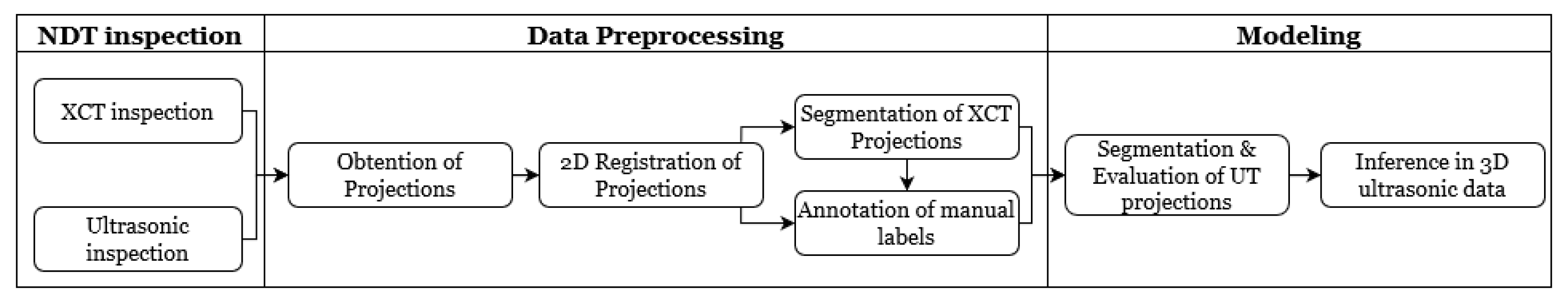
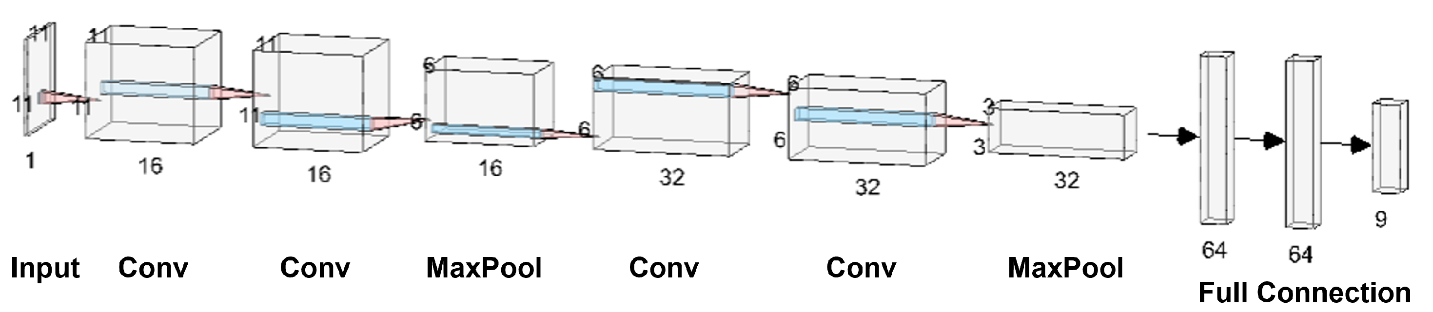
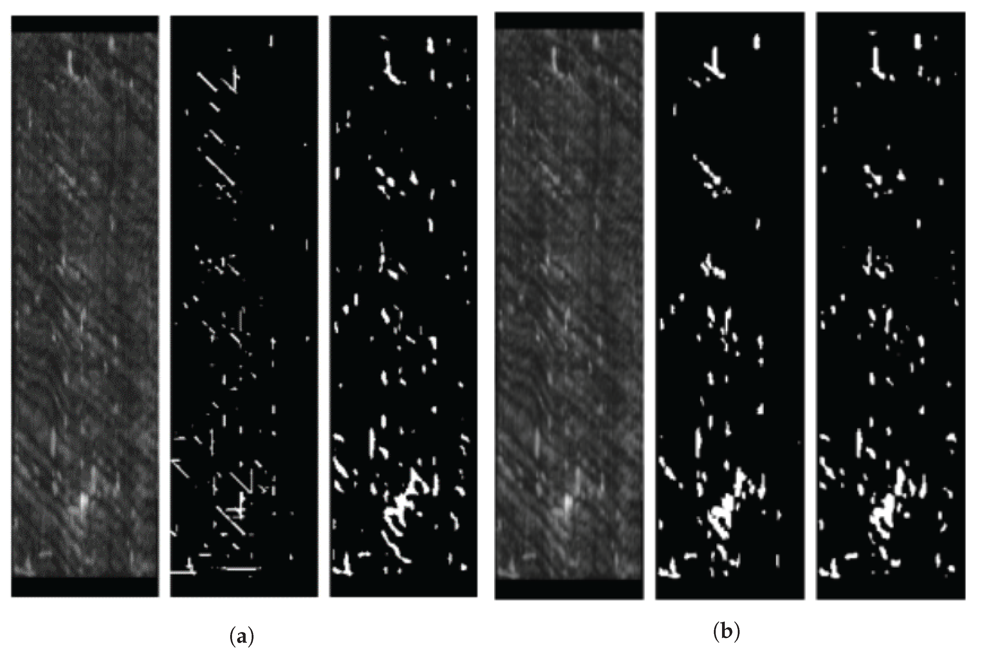
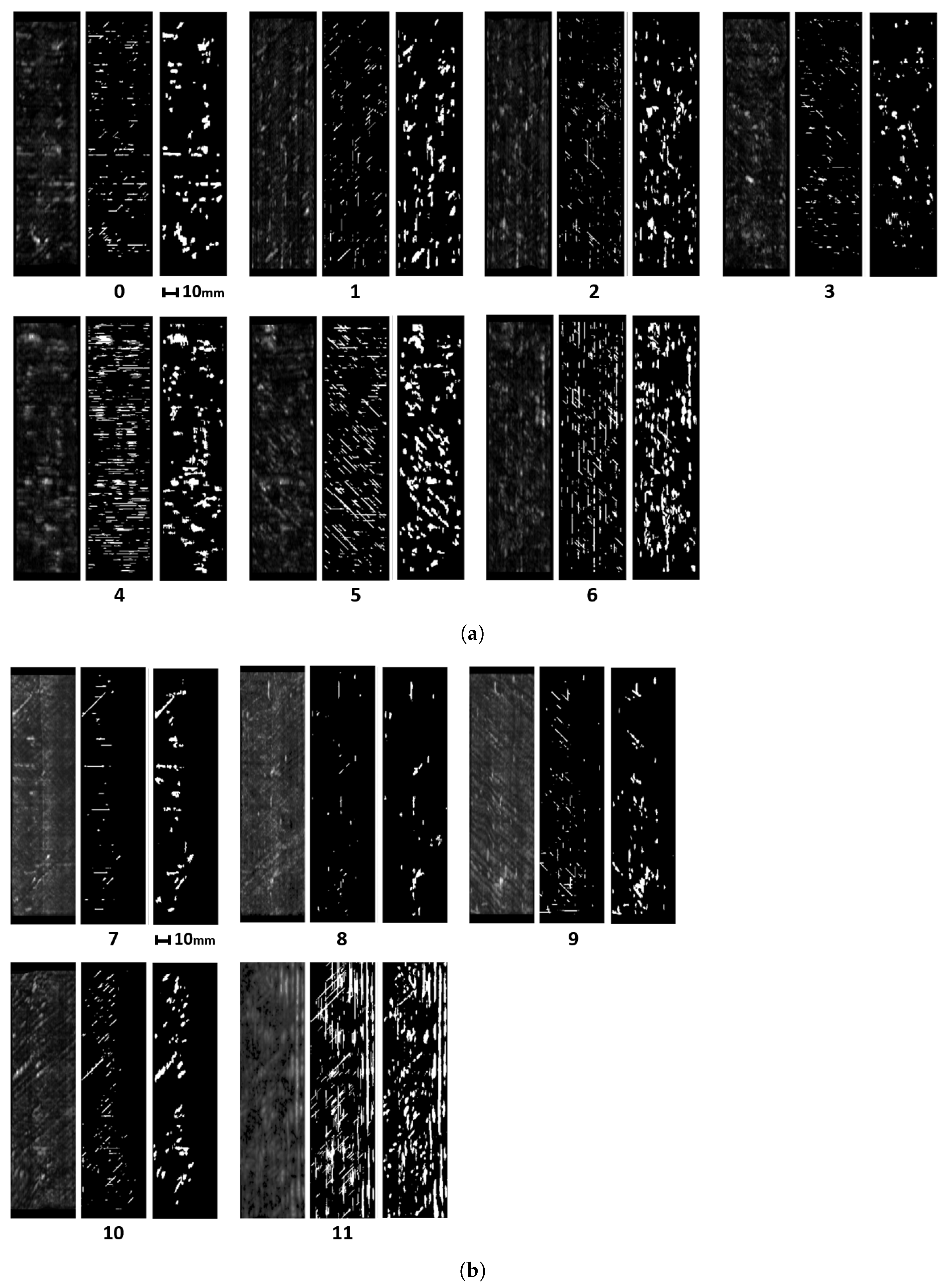
In this article, we develop a methodology for XCT and ultrasonic data fusion that trains a CNN to segment porosity. This would provide a 3D representation of porosity from ultrasonic data and improve the information on the impact of porosity on manufacturing, increasing quality and facilitating efficiency. To do this, phased array (PA) UT was used to obtain the best porosity images, XCT inspections were performed, and a labeled dataset of porosity defects was built and applied to train a convolutional neural network to segment the voids using UT images as input and XCT data as the ground truth. The dataset consists of several C-scans with different cases of void structures. The idea was to train a CNN on 2D cases, evaluated on a 2D test set, and use the trained network to infer ultrasonic 3D data as a sequence of C-scans, long the lines of the approach using B-scans reported in [15]. Experiments were performed on two 150 × 40 × 5 mm 3 CFRP coupons. The main contributions of the research are:
  • A methodology to use ultrasonic and XCT data and its application for porosity assessment, which is a use-case where UT data would not enable the formation of a supervised dataset;
  • the construction of a dataset of ultrasonic porosity images;
  • the optimization of phased array ultrasonic inspections enhances the detail level in the analysis of porosity, and void shape, size and distribution;
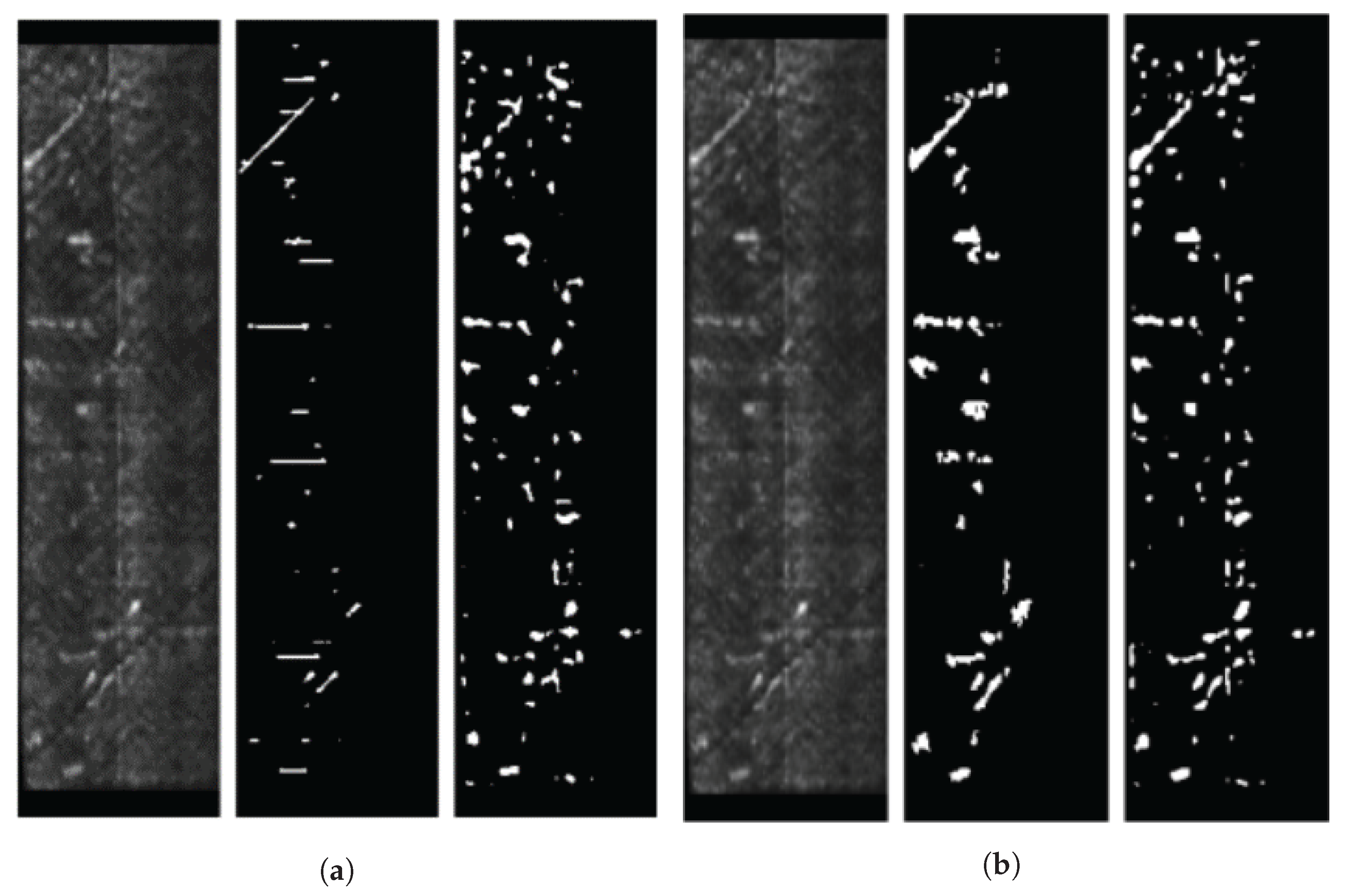
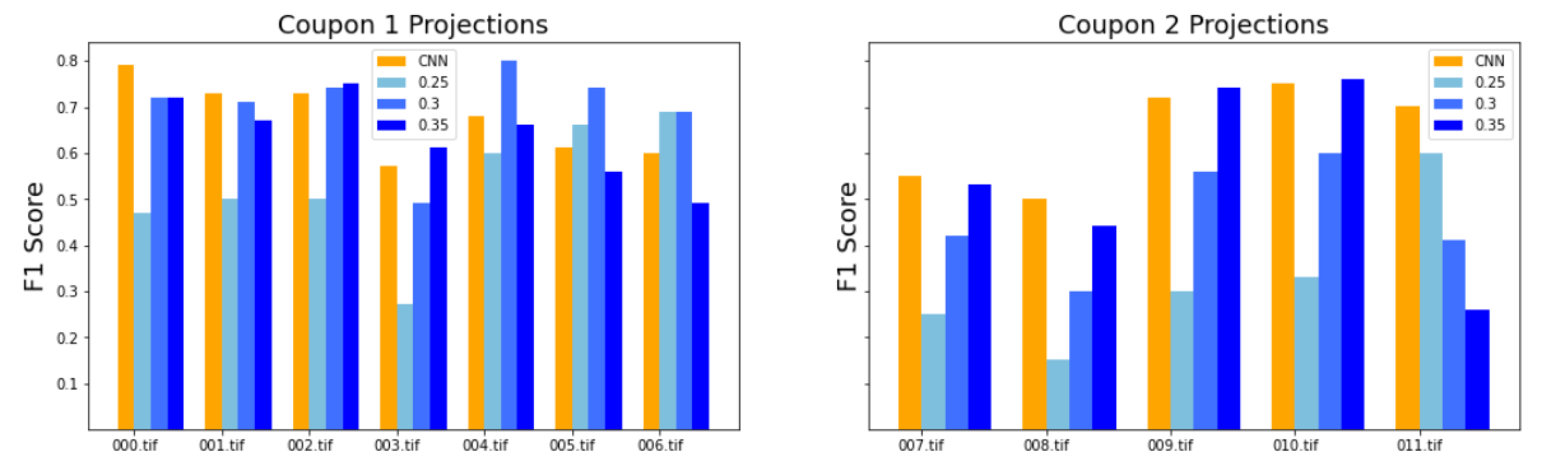
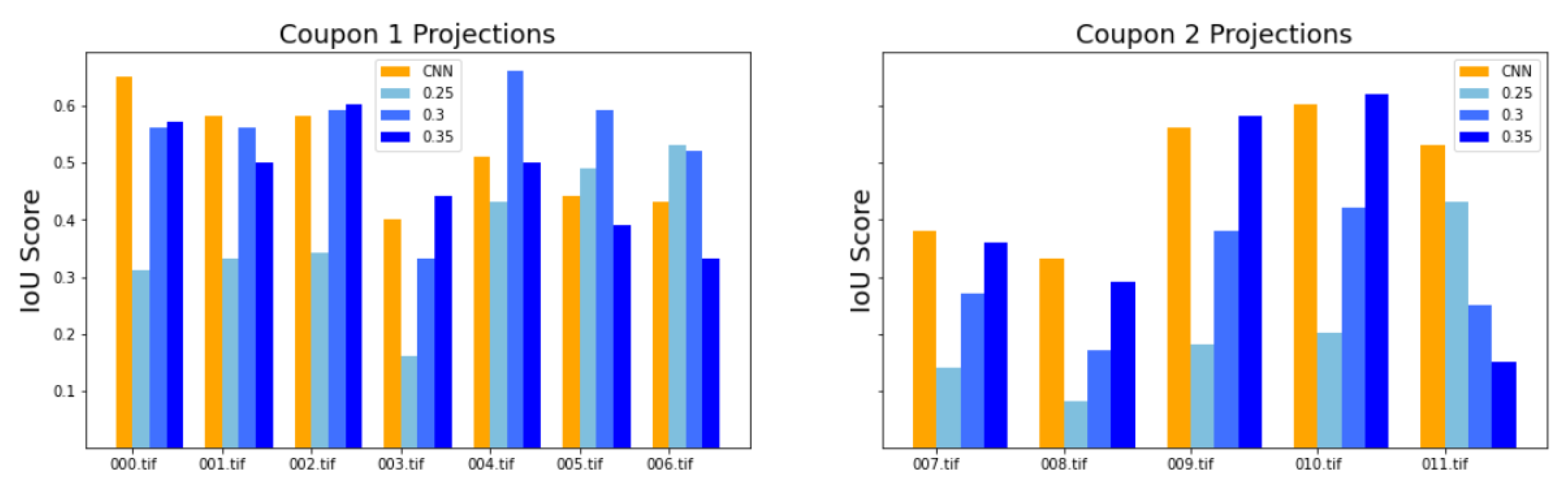
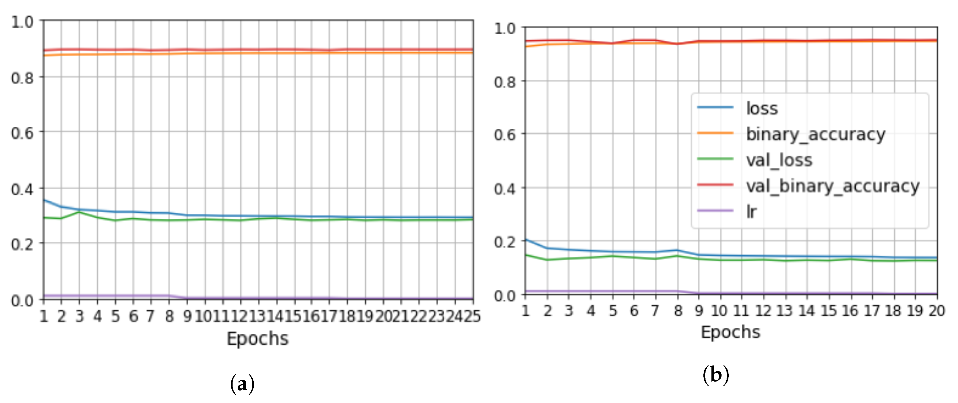
  • the evaluation of model performance depending on which data were used for training or testing, equal to an F1 of 0.6–0.7 and a IoU of 0.4–0.5 for the test data. Furthermore, the results proved to be robust, since the segmentation was equivalent for data that were part of the training and the test datasets in different training processes.

2. Materials and Methods

2.1. Materials

A thermoset carbon fiber panel was manufactured by stacking 16 layers in different directions 0 / 90 / ± 45 in out-of-autoclave modality at nonstandard temperature and pressure to produce porosity. It was then inspected using ultrasound, and two 150 × 40 × 5 mm 3 coupons were cropped from the panel in areas of the C-scan with variable attenuation values.

2.2. Methodology

Our approach to ultrasonic image segmentation was to apply supervised machine learning. To do this, we propose the use of a CNN, whose performance is compared to thresholds at different gray-levels. The aim is to develop a pipeline where 2D images from the PA are the neural network input, whose output is a 2D segmentation of any voids that they contain. Therefore, 3D volumes are treated as a collection of 2D images. Figure 1 shows an overview of the methodology. Figure 1 illustrates an overview of the methodology.
The proposed solution is to train a CNN with pairs of 2D ultrasound-XCT registered projections. Since we only have access to the data of two coupons, the data on one coupon are used for training, and the data on the other one are used for testing, and vice versa. Two different labels are explored as the ground truth: XCT data and manually defined labels based on the combination of the XCT and ultrasonic projections. The model performance metrics are calculated on the 2D test data set to measure the similarity of the neural network prediction to each of the ground truth sources. Once the model has been trained, it can be used on a 3D volume to predict porosity slice by slice. Because there were no labelled data, an evaluation based on error metrics was not feasible. Therefore, a visual comparison was performed to explore the differences in porosity prediction in the 3D volume.

2.2.1. NDT Inspections: XCT and Ultrasonic Phased Array

The two coupons were inspected by X-ray computed tomography with a voxel resolution equal to approximately 20 μ m. Local image thresholding using Sauvola processing methods in ImageJ was accurate enough to segment the voids, resulting in a binary volume with values of 1 for the voids and 0 for the material. Compared to the UT, the XCT was accurate enough for the segmented volume to be considered as the ground truth.
UT was performed using a 10 MHz linear array with a lens passively focusing the ultrasonic beam to improve its resolution. The tests were performed in immersion with Sitau ultrasonic equipment (Dasel, Spain). The passive direction of the array ran parallel to the major axis of the coupons, and mechanical scanning was performed in this direction with an optical encoder to measure displacement. The imaging mode was pulse-echo linear scan using a 32-element aperture, the pitch between elements was equal to 0.3 mm. Two parallel scans were required to inspect the width of each coupon (40 mm), which were then manually concatenated. This resulted in a 3D volume with an approximate size of 241 × 120 × 1352 voxels. The ultrasonic volume was rescaled to approximately 470 × 120 × 1352 to account for the influence of pitch.

2.2.2. Data Preprocessing

Obtention of Projection Images

The approach to UT-XCT volume registration was a 2D image registration of projections. During a pre-processing step, both volumes were manually aligned in the 3D space. The XCT projections were the result of the summation of several consecutive images (parallel to the composite surface) at different depths in the volume, whereas the maximum operator was used to obtain the projections at different depths in the US volume (Equation (1) defines the determination of a projection). The number of images to be included in each projection (k parameter) was manually selected to identify sufficient similar structures in the XCT and US projections. The process is defined below.
  • Let I = {1,...,l} denote the indices of the rows of a matrix A.
  • Let J = {1,...,m} denote the indices of the columns of matrix A
  • Let K = {1,...,n} denote the indices of the slices of matrix A
  • I, J, K are oriented to the height, width and thickness of the coupon, respectively
  • Let a i , j , k denote the value of the element A[i, j, k]
  • Let F be the summation operation in the case of XCT. The maximum operation in the case of the ultrasonic data
    p r o j e c t i o n = U i j = F ( a i j ) k = k 1 k 2 , i = 1 , , l j = 1 , , m ; k 1 and k 2 found experimentally .
The summation operation was found to be better suited for XCT because it highlights regions (white areas in Figure 2) and provides more microstructural information. After extracting all the images, histogram matching was applied to ultrasonic projections, and their pixel values were normalized in the interval [0,1]. This was performed to offset the differing intensity across the width due to ultrasound wave attenuation. This methodology output a total of 12 images for two 5 mm-thick coupons. The XCT images were scaled to fit the size of the PA projections, which was equal to 470 × 120 mm.

2D Registration of Projections

The registration was carried out on each pair of images. The XCT projection was used as a reference, and the ultrasonic projection as a moving image. We tested several automatic methods, and, as shown in Figure 2, the use of manually placed landmarks in common structures yielded the best results. The main obstacle to automated registration was that equivalent keypoints in the image pairs could not be identified automatically. The image registration algorithm is detailed in [36].

Labels

The registration was performed on gray-level XCT projections. The XCT-label projections were obtained through the segmentation of the gray-level XCT projections, which was performed using the local segmentation Sauvola filter algorithm (implemented in ImageJ).
A second labeling was performed as a result of the resolution differences between XCT and UT, which is explained in the discussion. To perform manual annotation, the registered projections of XCT and UT were superimposed, and the annotation was performed based on human criteria.

2.2.3. Modeling

Segmentation of UT Projections

The results of the convolutional neural network for image segmentation were compared to the performance of more conventional segmentation algorithms.
  • Global thresholds: different values for global segmentation of the projections were applied. The pixel values of the ultrasonic projections were normalized between [0, 1], and the thresholds were in the range [0.25, 0.4] with a 0.05 step. We also explored local segmentation algorithms such as Sauvola, but their results were found to be too noisy.
  • Network architecture: the network is a slightly modified version of the one shown in [37]. The hyperparameters are shown in Table 1. The proposed network has four convolutional layers with two max-pooling layers and three FC layers. The network architecture is illustrated in Figure 3. It was trained from scratch using extracted patches. Convolutional layers have a 3 × 3 kernel, stride 1, and no padding. Max pooling is performed with a 2 × 2 window and stride 2. All the hidden layers, except the output units, are equipped with rectified linear units (ReLU).
We also explored local segmentation algorithms such as Sauvola, but their results were found to be too noisy.

Training and Testing

In a situation where there are multiple labels, the output units are not necessarily exclusive. This means that there can be more than one positive output at the same time. To handle this scenario, the binary cross-entropy is utilized in the loss function. The binary cross-entropy is defined as:
L = 1 N i = 1 N y i log ( y i ^ ) + ( 1 y i ) log ( 1 y i ^ )
where N is the number of samples in the dataset, y i is the true label of the ith sample (either 0 or 1), y i ^ is the predicted probability of the ith sample belonging to the positive class (being a void), and log is the natural logarithm. No regularization was used in the network.
Data augmentation consisting uniquely in rotation of the training dataset was used. The dropout technique is an easy and efficient way to prevent overfitting. While training a neural network, some hidden neurons are randomly assigned a value of zero. This technique is applied to the first two fully connected (FC) layers, and the dropout ratio is set to 0.5. Weights in convolutional layers and FC layers are initialized using the Xavier method. Adam is adopted as the optimizer with a learning rate set to 0.01 and decaying to 0.002 from the ninth epoch onwards. The batch size for each iteration is set to 1256.

Evaluation

As mentioned under the methodology, the evaluation was performed on a set of 2D projections (see Figure 1). Using this approach, it is possible to calculate precision ( P r ) , recall ( R e ) , F1 score ( F 1 ) , and intersection over union (IoU), which are defined as follows.
P r = T P T P + F P R e = T P T P + F N F 1 = T P 2 T P + F N + F P I o U = T P T P + F N + F P
Being
  • False positive (FP): negative class predicted as positive.
  • True positive (TP): positive class predicted as positive.
  • True negative (TN): negative class predicted as negative.
  • False negative (FN): negative class predicted as positive.

2.3. Tools

Different open source software have been used along the project, namely TensorFlow, Fiji, Scikit-image, Jupiter Lab, Matplotlib, NumPy, Python-pillow and Napari [38,39,40,41,42,43,44,45].

3. Results

3.1. Dataset

The dataset (from UT and XCT data) of each coupon is composed of projections containing a widthwise portion (slab) of the material. Due to the natural differences between the coupons, seven pairs of projections were obtained for Coupon 1 and five for Coupon 2. Each of the XCT/UT projections were obtained as explained in the methodology. The XY size of each projection was approximately 470 × 120 pixels (each pixel is about 1 mm 2 ).
The dataset is shown in the Appendix B. The projections for each coupon are ordered from the closest to the front surface to the closest to the back surface. Several variations between projections, such as void orientation and size, sharpness, and location of noisy structures, are appreciable. A vast majority of the voids segmented in the XCT can be related to bright structures in the ultrasonic data. Thus, the preprocessing stage enables the formation of a dataset for defect segmentation.

3.2. CNN Training

Figure 4 and Figure 5 show examples of the results of applying the CNN, Figure 6 contains the validation curves for the networks trained with each label type, and Table 2 and Table 3 show the evaluation metrics using projections of Coupon 1 as training data and projections of Coupon 2 as test data. The Appendix A reports the results of training on projections of Coupon 2 and testing on Coupon 1. Table 4 shows the mean of the evaluation metrics for all projections of the dataset in the case of manual annotations as ground truth.

Comparison of Segmentation Algorithms along the Dataset

The measured F1 evaluation metric for the segmentation results on manual labels for each threshold and the CNN are shown in Figure 7, the IoU in Figure 8.

4. Discussion

4.1. Preprocessing

The phased array amplitude C-scans enables the detection and measurement of voids down to one hundred μ m thin. The human eye can establish clear correlations between void defects in XCT and C-scans. The obtention of projections was motivated as a way to deal with the mismatch in the depth dimension between the ultrasonic and XCT volumes. In this sense, the similarity in the porosity between both sources is clear. The way projections are obtained highlights the void structures, but it also strengthens echoes caused by resin areas or other structures. Although the equalization process of the ultrasonic projections compensates for the attenuation along the thickness, probably other techniques, such as an adaptive time gain (TGC) during inspection, may improve the results.

4.2. Registration

We found that 3D registration was not accurate enough to train the CNN, mostly due to the mentioned mismatch in the depth dimension. The automation of registration is primarily limited by the difficulty in automatically detecting common salient structures, structural descriptors, or any metric of statistical dependency for both data sources. However, once the algorithm developed in [36] counts with enough common keypoints between the 2D images, registration is successful. A possible future line of research would be to explore whether deep learning models are able to find similar keypoints, for which purpose our annotated data could be used.

4.3. Evaluation and Labels

Two different image labels were used as ground truths in two independent training sessions. The use of XCT projections as labels is the most straightforward training method for a CNN. However, each source has different resolutions, which results in data that are not adequate for the classification task. On this ground, we also used manual labeling. Figure 9 illustrates the differences in labeling porosity between the XCT projections (through automatic local thresholding) and the manual labels in US projections. Bright pixels account for internal echoes, which can be caused by defects caused by porosity or by the internal microstructure of the composite, for instance, resin pockets. The aim of the network is to segment the defect echoes. If XCT labels are used, there is only a small difference between void and nearby pixels. The different resolutions of the NDT techniques account for this behavior. Manual labeling is performed assuming that all bright pixels within a specified region should be produced by the voids. As a result of the above resolution effect, the precision, recall, and F1 results measured using the manual labels are double that of the XCT labels.
Manual labels are the best option for training the network. However, XCT labels are still needed to perform manual labeling. In other words, the XCT ground truth is required to single out echoes produced by defects from those produced by other factors such as microstructure or noise.

4.4. Segmentation Results

The evaluation metrics in Table 4 shows that the CNN performs better than any threshold in average for the entire dataset. The values of F1 and IoU around 0.66 and 0.50 are not enough to be used in a production environment. Despite this, the distance to production-level results is not far. Strategies such as the ones mentioned in the state-of-the-art, combining A-scan signal data with C-scans and a bigger dataset may raise the performance level to the requirements. In addition, the evaluation of the models in object detection metrics remains a future work.
As Figure 7 and Figure 8 show, the performance varies in a range up to 0.2 in F1 and IoU across the different projections. The CNN fails with respect to challenging segmentation cases, such as projections near to the front surface, e.g., the two first projections in the Coupon 2 dataset and the last one in Coupon 1 (see dataset in the appendix), which are noisier, or in resin-rich pocket regions. The orientation of the voids played a role as well, in projections such as 3 and 4 with more presence of horizontal and diagonal aligned voids the metrics decreased. The visual evaluation after the 3D prediction confirmed these challenging cases: resin structures, slices near the front or back surfaces, showed echoes that were indistinguishable from the defects. This is a future line of research, where possible solutions include improving the signal-to-noise ratio, deconvolution of the A-scan signals, further optimization of the ultrasonic imaging, and the integration of additional features of the ultrasonic signal.
A key result is the robustness of the training, irrespective of whether the CNN is trained on the data of Coupon 1 or Coupon 2, the training and test results are equivalent. In other words, the evaluation metrics are equivalent when the projections of Coupon 1 are used for training to when they are used in testing. The network appears to be able to interpret where segmentation must be performed and is consistent even if the training and test data roles are inverted.

5. Conclusions and Future Work

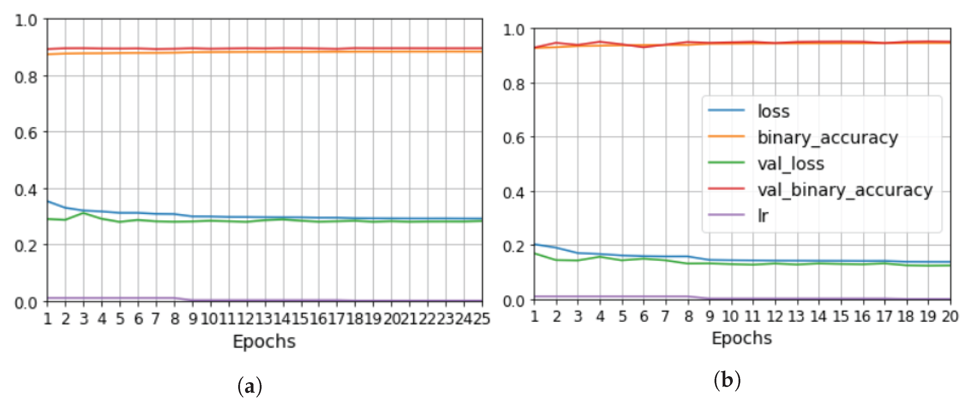
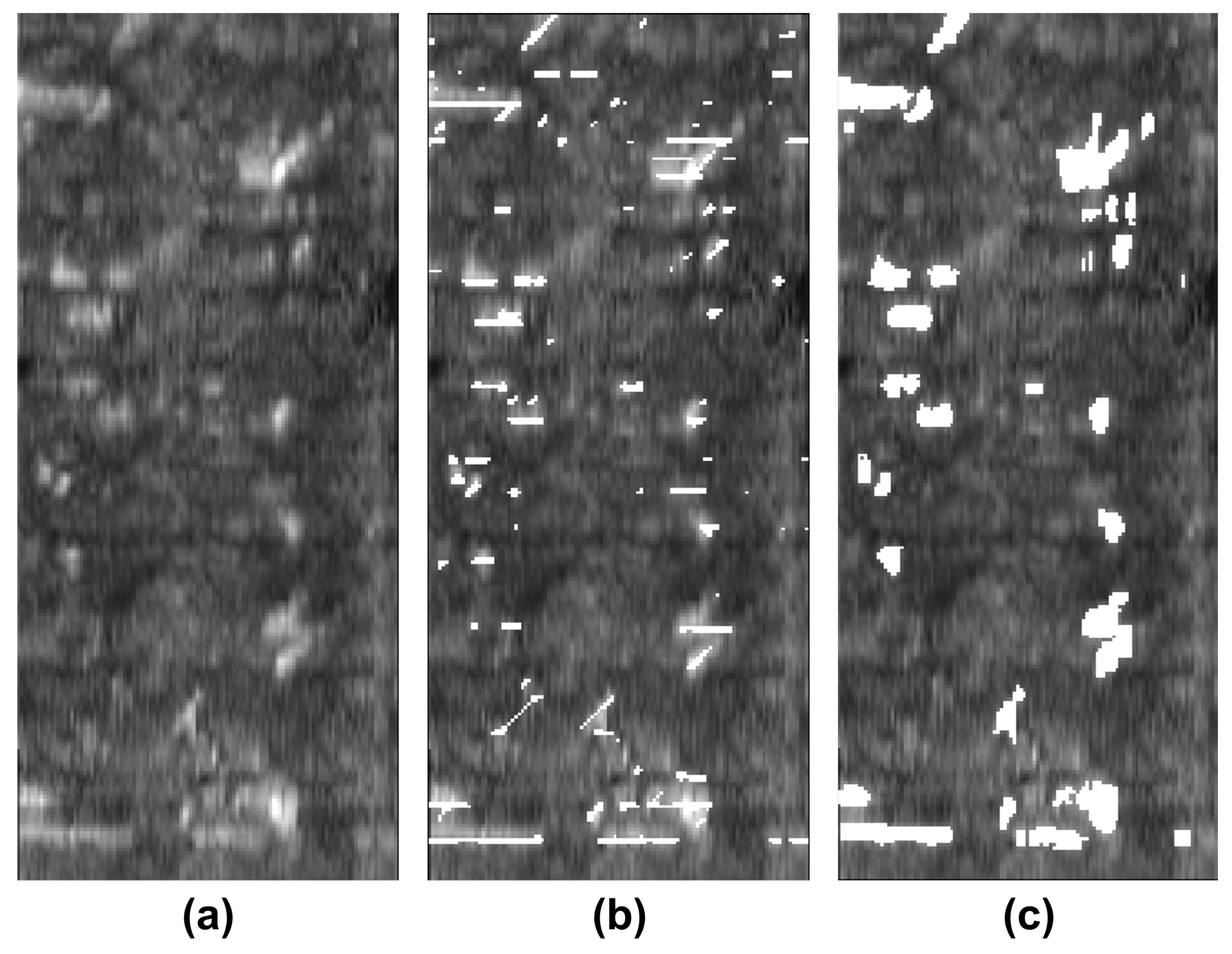
We developed a methodology to semi-automatically segment defects in 3D ultrasonic data using a convolutional neural network (CNN). The methodology consists of X-ray computed tomography and phased-array ultrasonic testing data fusion. Supervised classification was then used to train the CNN with 2D images. The use of this approach makes it possible to measure evaluation metrics such as precision, recall, F1 and IoU. The CNN results were compared to the outcomes of applying global thresholds to the phased array. According to the metrics implemented, CNN clearly outperformed the global threshold.
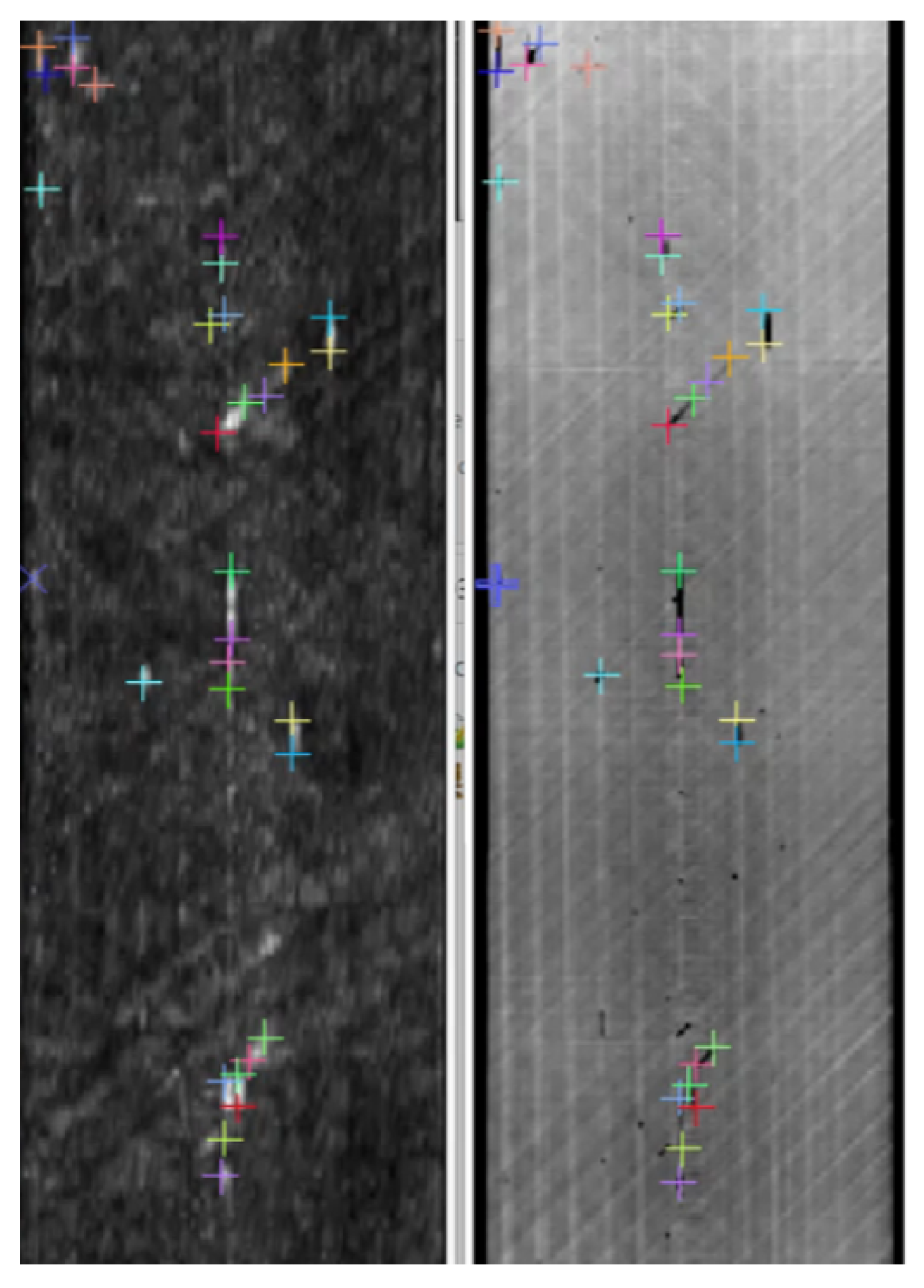
One of the most challenging tasks is data fusion. The proposed solution is an image registration process for 2D images output by each technique, as 3D registration was found not to be accurate enough to train the CNN. In the absence of an algorithm to find common keypoints or any similarity measure between the two data sources, however, registration is not fully automated. This is a future line of work, where the application of deep learning based on the manually annotated data reported here could prove to be useful.
We explored the use of two ground truths: XCT segmented voids and manual labels. The use of the XCT labels was found to output data that were too noisy for CNN training, and manual labels provided more robust training. The evaluation metrics for manual labels were twice as good. The network results—an F1 for test data equal to 0.63 and IoU equal to 0.5—were better than outcomes for the global thresholds. However, CNN is not able to distinguish between echoes produced by defects such as porosity and echoes produced by microstructural elements such as resin-rich areas. Future works should improve the signal-to-noise ratio, increase the dataset, and integrate more information from ultrasonic signals and C-scan representations.

Author Contributions

Conceptualization, J.-I.C. and F.S.; methodology, J.-I.C., G.C., J.C., E.M. and C.G.-M.; software, J.-I.C.; validation, E.M. and G.C.; formal analysis, J.-I.C.; investigation, J.-I.C.; resources, E.M. and J.C.; data curation, J.-I.C.; writing—review and editing, J.-I.C., F.S., G.C. and E.M.; visualization, J.-I.C.; supervision, E.M. and F.S.; project administration, E.M. and F.S.; funding acquisition, E.M. All authors have read and agreed to the published version of the manuscript.

Funding

The research leading to these results has received funding from Madrid region under programme S2018/NMT-4381-MAT4.0-CM project.

Institutional Review Board Statement

Not applicable.

Informed Consent Statement

Not applicable.

Data Availability Statement

Two dataset from this reasearch are available: the unregistered set of 2D UT/XCT images with its associated manually annotated keypoints, and the set of ultrasonic, XCT, and manual labels images used in the training of the CNN. Everything will be provided openly. They can be shared upon request as well with explanations.

Acknowledgments

Special thanks to Julen Barriga Valles, his work during his bachelor final project helped in the development of the CNN network.

Conflicts of Interest

The authors declare no conflict of interest.

Abbreviations

The following abbreviations are used in this manuscript:
MDPIMultidisciplinary Digital Publishing Institute
DOAJDirectory of open access journals
NDTNon-destructive testing
UTUltrasonic testing
XCTX-ray computed tomography
CNNConvolutional neural networks

Appendix A. Results for Training in Data of Coupon 2, and Test in Coupon 1

Table A1. Training evaluation metrics.
XCT LabelsManual Labels
Avg Training Precision:0.320.51
Avg Training Recall:0.450.89
Avg Training F1:0.250.62
Avg Training IoU:0.140.62
Table A2. Test evaluation metrics.
XCT LabelsManual Labels
Avg Test Precision:0.290.72
Avg Test Recall:0.360.78
Avg Test F1:0.290.73
Avg Training IoU:0.170.62
Figure A1. Training and validation curves for the networks trained on each type of labels. (a) Network trained with XCT labels. (b) Network trained with manual labels.
Applsci 13 05933 g0a1

Appendix B. Dataset of Projections

Figure A2. Dataset of projections and their imageID. From left to right: Ultrasonic, XCT labels, and manual labels images. (a) Projections obtained from coupon 1. From left to right: Ultrasonic, XCT labels, and manual labels images. (b) Projections obtained from coupon 2.
Applsci 13 05933 g0a2

References

  1. Szegedy, C.; Liu, W.; Jia, Y.; Sermanet, P.; Reed, S.; Anguelov, D.; Erhan, D.; Vanhoucke, V.; Rabinovich, A. Going Deeper with Convolutions. arXiv 2014, arXiv:1409.4842. [Google Scholar]
  2. Simonyan, K.; Zisserman, A. Very Deep Convolutional Networks for Large-Scale Image Recognition. arXiv 2015, arXiv:1409.1556. [Google Scholar]
  3. He, K.; Zhang, X.; Ren, S.; Sun, J. Deep Residual Learning for Image Recognition. arXiv 2015, arXiv:1512.03385. [Google Scholar]
  4. Krizhevsky, A.; Sutskever, I.; Hinton, G.E. ImageNet Classification with Deep Convolutional Neural Networks. Commun. ACM 2017, 60, 84–90. [Google Scholar] [CrossRef]
  5. Vaswani, A.; Shazeer, N.; Parmar, N.; Uszkoreit, J.; Jones, L.; Gomez, A.N.; Kaiser, L.; Polosukhin, I. Attention Is All You Need. arXiv 2017, arXiv:1706.03762. [Google Scholar]
  6. Ren, S.; He, K.; Girshick, R.; Sun, J. Faster R-CNN: Towards Real-Time Object Detection with Region Proposal Networks. arXiv 2016, arXiv:1506.01497. [Google Scholar] [CrossRef] [PubMed]
  7. Redmon, J.; Divvala, S.; Girshick, R.; Farhadi, A. You Only Look Once: Unified, Real-Time Object Detection. arXiv 2016, arXiv:1506.02640. [Google Scholar]
  8. He, K.; Gkioxari, G.; Dollár, P.; Girshick, R. Mask R-CNN. arXiv 2018, arXiv:1703.06870. [Google Scholar]
  9. Xiao, H.; Chen, D.; Xu, J.; Guo, S. Defects Identification Using the Improved Ultrasonic Measurement Model and Support Vector Machines. NDT E Int. 2020, 111, 102223. [Google Scholar] [CrossRef]
  10. Ye, J.; Toyama, N. Benchmarking Deep Learning Models for Automatic Ultrasonic Imaging Inspection. IEEE Access 2021, 9, 36986–36994. [Google Scholar] [CrossRef]
  11. Latête, T.; Gauthier, B.; Belanger, P. Towards Using Convolutional Neural Network to Locate, Identify and Size Defects in Phased Array Ultrasonic Testing. Ultrasonics 2021, 115, 106436. [Google Scholar] [CrossRef] [PubMed]
  12. Medak, D.; Posilovic, L.; Subasic, M.; Budimir, M.; Loncaric, S. Automated Defect Detection From Ultrasonic Images Using Deep Learning. IEEE Trans. Ultrason. Ferroelectr. Freq. Control 2021, 68, 3126–3134. [Google Scholar] [CrossRef] [PubMed]
  13. Tan, M.; Pang, R.; Le, Q.V. EfficientDet: Scalable and Efficient Object Detection. arXiv 2020, arXiv:1911.09070. [Google Scholar]
  14. Lin, T.Y.; Goyal, P.; Girshick, R.; He, K.; Dollár, P. Focal Loss for Dense Object Detection. arXiv 2018, arXiv:1708.02002. [Google Scholar]
  15. Medak, D.; Posilovic, L.; Subasic, M.; Budimir, M.; Loncaric, S. Deep Learning-Based Defect Detection From Sequences of Ultrasonic B-Scans. IEEE Sens. J. 2022, 22, 2456–2463. [Google Scholar] [CrossRef]
  16. Virkkunen, I.; Koskinen, T.; Jessen-Juhler, O.; Rinta-aho, J. Augmented Ultrasonic Data for Machine Learning. J. Nondestruct. Eval. 2021, 40, 4. [Google Scholar] [CrossRef]
  17. Cantero-Chinchilla, S.; Wilcox, P.D.; Croxford, A.J. A Deep Learning Based Methodology for Artefact Identification and Suppression with Application to Ultrasonic Images. NDT E Int. 2022, 126, 102575. [Google Scholar] [CrossRef]
  18. Meng, M.; Chua, Y.J.; Wouterson, E.; Ong, C.P.K. Ultrasonic Signal Classification and Imaging System for Composite Materials via Deep Convolutional Neural Networks. Neurocomputing 2017, 257, 128–135. [Google Scholar] [CrossRef]
  19. Li, C.; He, W.; Nie, X.; Wei, X.; Guo, H.; Wu, X.; Xu, H.; Zhang, T.; Liu, X. Intelligent Damage Recognition of Composite Materials Based on Deep Learning and Ultrasonic Testing. AIP Adv. 2021, 11, 125227. [Google Scholar] [CrossRef]
  20. Qiao, S.; Chen, L.C.; Yuille, A. DetectoRS: Detecting Objects with Recursive Feature Pyramid and Switchable Atrous Convolution. arXiv 2020, arXiv:2006.02334. [Google Scholar]
  21. Girshick, R.; Donahue, J.; Darrell, T.; Malik, J. Rich Feature Hierarchies for Accurate Object Detection and Semantic Segmentation. arXiv 2014, arXiv:1311.2524. [Google Scholar]
  22. Smith, R.A. President, BINDT. Workshop on NDT and SHM Requirements for Aerospace, Composites. Available online: https://www.bindt.org/admin/Downloads/2016 (accessed on 10 January 2022).
  23. Sket, F.; Seltzer, R.; Molina-Aldareguía, J.; Gonzalez, C.; LLorca, J. Determination of Damage Micromechanisms and Fracture Resistance of Glass Fiber/Epoxy Cross-Ply Laminate by Means of X-ray Computed Microtomography. Compos. Sci. Technol. 2012, 72, 350–359. [Google Scholar] [CrossRef]
  24. Mutiargo, B. Evaluation of X-Ray Computed Tomography (CT) Images of Additively Manufactured Components Using Deep Learning. In Proceedings of the 3rd Singapore International Non-Destructive Testing Conference and Exhibition (SINCE2019), Singapore, 12 May 2019; p. 9. [Google Scholar]
  25. Hernández, S.; Sket, F.; Molina-Aldareguı´a, J.; González, C.; LLorca, J. Effect of Curing Cycle on Void Distribution and Interlaminar Shear Strength in Polymer-Matrix Composites. Compos. Sci. Technol. 2011, 71, 1331–1341. [Google Scholar] [CrossRef]
  26. Smith, R.A.; Nelson, L.J.; Mienczakowski, M.J.; Wilcox, P.D. Ultrasonic Tracking of Ply Drops in Composite Laminates. In Proceedings of the 42nd Annual Review of Progress in Quantitative Nondestructive Evaluation: Incorporating the 6th European-American Workshop on Reliability of NDE, Minneapolis, MN, USA, 26–31 July 2016; p. 050006. [Google Scholar] [CrossRef]
  27. Ma, L.; Ma, T.; Liu, R.; Fan, X.; Luo, Z. Toward Fast, Flexible, and Robust Low-Light Image Enhancement. In Proceedings of the 2022 IEEE/CVF Conference on Computer Vision and Pattern Recognition (CVPR), New Orleans, LA, USA, 18–24 June 2022; pp. 5627–5636. [Google Scholar] [CrossRef]
  28. Liu, Y.; Yan, Z.; Tan, J.; Li, Y. Multi-Purpose Oriented Single Nighttime Image Haze Removal Based on Unified Variational Retinex Model. IEEE Trans. Circuits Syst. Video Technol. 2023, 33, 1643–1657. [Google Scholar] [CrossRef]
  29. Sparkman, D.; Wallentine, S.; Flores, M.; Wertz, J.; Welter, J.; Schehl, N.; Dierken, J.; Zainey, D.; Aldrin, J.; Uchic, M. A Supervised Learning Approach for Prediction of X-Ray Computed Tomography Data from Ultrasonic Testing Data. In Proceedings of the 45th Annual Review of Progress in Quantitative Nondestructive Evaluation, Burlington, VT, USA, 15–19 July 2019; Volume 38, p. 030002. [Google Scholar] [CrossRef]
  30. Birt, E.A.; Smith, R.A. A Review of NDE Methods for Porosity. Insight-Non-Destr. Test. Cond. Monit. 2004, 46, 681–686. [Google Scholar] [CrossRef]
  31. Ding, S.; Jin, S.; Luo, Z.; Liu, H.; Chen, J.; Lin, L.; Laboratory, E. Investigations on Relationship between Porosity and Ultrasonic Attenuation Coefficient in CFRP Laminates Based on RMVM. In Proceedings of the 7th International Symposium on NDT in Aerospace, Bremen, Germany, 16–18 November 2015. [Google Scholar]
  32. Lin, L.; Luo, M.; Tian, H. Experimental Investigation on Porosity of Carbon Fiber-Reinforced Composite Using Ultrasonic Attenuation Coefficient. In Proceedings of the 17th World Conference on Nondestructive Testing, Shanghai, China, 25–28 October 2008; p. 9. [Google Scholar]
  33. Mehdikhani, M.; Gorbatikh, L.; Verpoest, I.; Lomov, S.V. Voids in Fiber-Reinforced Polymer Composites: A Review on Their Formation, Characteristics, and Effects on Mechanical Performance. J. Compos. Mater. 2018, 53, 1579–1669. [Google Scholar] [CrossRef]
  34. Bhat, S.S.; Zhang, J.; Larrosa, N. Sizing Limitations of Ultrasonic Array Images for Non-Sharp Defects and Their Impact on Structural Integrity Assessments. Theor. Appl. Fract. Mech. 2022, 122, 103625. [Google Scholar] [CrossRef]
  35. Chapon, A.; Pereira, D.; Toews, M.; Belanger, P. Deconvolution of Ultrasonic Signals Using a Convolutional Neural Network. Ultrasonics 2021, 111, 106312. [Google Scholar] [CrossRef]
  36. Arganda-Carreras, I.; Sorzano, C.O.S.; Marabini, R.; Carazo, J.M.; Ortiz-de-Solorzano, C.; Kybic, J. Consistent and Elastic Registration of Histological Sections Using Vector-Spline Regularization. In Computer Vision Approaches to Medical Image Analysis; Hutchison, D., Kanade, T., Kittler, J., Kleinberg, J.M., Mattern, F., Mitchell, J.C., Naor, M., Nierstrasz, O., Pandu Rangan, C., Steffen, B., et al., Eds.; Springer: Berlin/Heidelberg, Germany, 2006; Volume 4241, pp. 85–95. [Google Scholar] [CrossRef]
  37. Fan, Z.; Wu, Y.; Lu, J.; Li, W. Automatic Pavement Crack Detection Based on Structured Prediction with the Convolutional Neural Network. arXiv 2018, arXiv:1802.02208. [Google Scholar]
  38. Abadi, M.; Agarwal, A.; Barham, P.; Brevdo, E.; Chen, Z.; Citro, C.; Corrado, G.S.; Davis, A.; Dean, J.; Devin, M.; et al. TensorFlow: Large-Scale Machine Learning on Heterogeneous Distributed Systems. arXiv 2015, arXiv:1603.04467. [Google Scholar]
  39. Schindelin, J.; Arganda-Carreras, I.; Frise, E.; Kaynig, V.; Longair, M.; Pietzsch, T.; Preibisch, S.; Rueden, C.; Saalfeld, S.; Schmid, B.; et al. Fiji: An Open-Source Platform for Biological-Image Analysis. Nat. Methods 2012, 9, 676–682. [Google Scholar] [CrossRef] [PubMed]
  40. van der Walt, S.; Schönberger, J.L.; Nunez-Iglesias, J.; Boulogne, F.; Warner, J.D.; Yager, N.; Gouillart, E.; Yu, T. Scikit-Image: Image Processing in Python. PeerJ 2014, 2, e453. [Google Scholar] [CrossRef] [PubMed]
  41. Hunt, M.; Jupyter Lab. nanoHUB. 2018. Available online: https://nanohub.org/resources/jupyterlab60/about (accessed on 5 May 2020).
  42. Caswell, T.A.; Droettboom, M.; Lee, A.; Hunter, J.; Firing, E.; Stansby, D.; Klymak, J.; Hoffmann, T.; Andrade, E.S.D.; Varoquaux, N.; et al. Matplotlib/Matplotlib: REL: V3.2.1. Zenodo. 2020. Available online: https://matplotlib.org/stable/users/project/citing.html (accessed on 4 June 2019).
  43. Oliphant, T.E. A Guide to NumPy. Available online: https://web.mit.edu/dvp/Public/numpybook.pdf (accessed on 25 January 2022).
  44. Kemenade, H.V.; Wiredfool; Murray, A.; Clark, A.; Karpinsky, A.; Gohlke, C.; Dufresne, J.; Nulano; Crowell, B.; Schmidt, D.; et al. Python-Pillow/Pillow 7.1.2. Zenodo. 2020. Available online: https://buildmedia.readthedocs.org/media/pdf/pillow/latest/pillow.pdf (accessed on 4 February 2019).
  45. Sofroniew, N.; Lambert, T.; Evans, K.; Nunez-Iglesias, J.; Solak, A.C.; Yamauchi, K.; Buckley, G.; Bokota, G.; Tung, T.; Freeman, J.; et al. Napari/Napari: 0.3.3. Zenodo. 2020. Available online: https://napari.org/stable/citing-napari (accessed on 12 May 2021).
Figure 1. Flow diagram of the methodology.
Applsci 13 05933 g001
Figure 2. Detail of a pair of projections illustrating the keypoints identifiying common voids.
Applsci 13 05933 g002
Figure 3. Diagram of the CNN structure. The leftmost image is the input patch with one channel. Other cubes indicate the feature maps obtained from convolution (Conv) or max pooling. All convolutional layers have a kernel of 3 × 3, stride 1 and zeros padding. Max pooling is performed with stride 2 over a 2 × 2 window.
Applsci 13 05933 g003
Figure 4. Results for projection 1 of test data (Coupon 2). (a) Ultrasonic projection, XCT ground truth, and predicted image. (b) Ultrasonic input, manual labels, and predicted image.
Applsci 13 05933 g004
Figure 5. Results for the projection 3 of test data. (a) Ultrasonic input, XCT ground truth, and predicted image. (b) Ultrasonic input, manual labels, and predicted image.
Applsci 13 05933 g005
Figure 6. Training and validation curves for the networks trained on each type of labels. (a) Network trained with XCT labels. (b) Network trained with manual labels.
Applsci 13 05933 g006
Figure 7. Comparison of F1 for the 0.25,0.3 and 0.35 global threshold segmentations applied to the US projection on a [0, 1] gray scale, and the CNN. In the case of the network, the value of F1 was obtained when the image formed part of the test dataset.
Applsci 13 05933 g007
Figure 8. Comparison of IoU for the 0.25,0.3 and 0.35 global threshold segmentations applied to the US projection on a [0, 1] gray scale, and the CNN. In the case of the network, the value of IoU was obtained when the image formed part of the test dataset.
Applsci 13 05933 g008
Figure 9. Detail of a projection illustrating the differences between the two labels used. (a) Ultrasonic input. (b) XCT labels superimposed. (c) Manual labels superimposed.
Applsci 13 05933 g009
Table 1. Table of hyperparatemers for each type of label.
LabelsRatioEpochhs
Manual112051
XCT62551
Table 2. Training evaluation metrics.
XCT LabelsManual Labels
Avg Training Precision:0.290.90
Avg Training Recall:0.420.53
Avg Training F1:0.310.66
Avg IoU:0.190.50
Table 3. Test evaluation metrics.
XCT LabelsManual Labels
Avg Test Precision:0.270.67
Avg Test Recall:0.490.72
Avg Test F1:0.270.67
Avg IoU:0.160.51
Table 4. Average evaluation metrics for the manually annotated labels and projections from the two coupons. In the case of the CNN, the metrics were obtained when the projections belong to the test dataset.
Avg. PrecisionAvg. RecallAvg. F1Avg. IoU
CNN0.740.650.660.50
Thr: 0.250.350.920.440.30
Thr: 0.30.580.790.600.44
Thr: 0.350.770.590.600.44
Thr: 0.40.860.390.490.34
Thr: 0.450.920.240.350.22
Disclaimer/Publisher’s Note: The statements, opinions and data contained in all publications are solely those of the individual author(s) and contributor(s) and not of MDPI and/or the editor(s). MDPI and/or the editor(s) disclaim responsibility for any injury to people or property resulting from any ideas, methods, instructions or products referred to in the content.

