Abstract
Sampled points on a measured surface are not evenly spaced on rectangular grids but, rather, have a more general quadrilateral geometry due to the perspective effect of the off-axis configuration, which is extensively utilized in phase measuring deflectometry (PMD). The current procedures for slope-to-wavefront integration results in reconstruction errors, which impact PMD to achieve a higher measurement accuracy. Due to the advantageous properties of the radial basis function (RBF) for irregular sampling and incomplete data, the quadrilateral geometry acquired by a CCD is first realized in this paper using the ray tracing method, which is used to obtain the actual measurement area and sampling interval in off-axis PMD instead of the area defined by the mathematical formula in the past when RBF was used. The RBF integration method is researched in this paper. The simulation and experiment show that RBF is a robust and higher accuracy algorithm for off-axis PMD. We further implement the RBF integration method to measure a crystal transparent element where an off-axis configuration is required.
1. Introduction
Phase measuring deflectometry (PMD) is a surface measurement technique for specular or transmitted objects that are commonly used in the processing and manufacturing of optical components, such as wafers, automobile window glass, and other products. PMD has shown the advantages of incoherence, large dynamic range, simple device, low cost, and comparable accuracy to interferometer [1,2,3,4], etc. Currently, it is attracting extensive interest in the field of surface measurement [5,6,7] of optics. In PMD, the phase-shifted sinusoidal fringe patterns are projected and reflected off the specular surface to obtain the slope of the surface under test. Although co-axis PMD can reduce the influence of systematic errors, the complexity of the measuring device is increased, and more importantly, there are scenarios where off-axis configuration is required, such as transparent element measurement with a binary pattern [8]. Generally, the off-axis configuration is widely adopted [9] when the sampling points on the measured surface are spaced on distorted quadrilateral grids instead of regular rectangular grids. This leads to a decrease in the accuracy of some slope-based reconstruction algorithms [10]. Modal methods [11,12], as a member of the broad family of slope-based surface reconstruction algorithms, can integrate the shape with the points as a whole using standard orthogonal polynomial fit. While zonal methods [13,14] integrate the positions of the points one by one at the location of the sampling points, they still cannot handle a case with irregular sampling points. In 2017, Mengyang Li et al. [15] proposed an improved zonal algorithm to address the issue of the aperture of the test optics that are not rectangular due to keystone distortion and occlusion, and even with an arbitrary sampling point distribution, the measurement accuracy still needs to be improved to meet higher requirements. In 2008, S. Ettl et al. [16] introduced the radial basis function, which combines Hermite interpolation for discrete data and allows irregularly shaped sampling ranges or sampling points to be taken at irregular intervals. After that, in 2015, Huang et al. [17] compared the RBF with other slope-based surface reconstruction algorithms in dealing with quadrilateral geometry. During their simulation, a rectangular mesh was mathematically deformed to generate a quadrilateral grid, and the comparison results showed the advantages of RBF in handling quadrilateral geometry. Meanwhile, Ren et al. [18,19] also simulated the quadrilateral geometry by setting distortion coefficients for the camera, and Huang et al. [20] combined three distorted meshes (random error, distortion, and trapezoid) to generate a new quadrilateral grid. However, both the actual position of the camera or the components and the surface shape of the optics to be measured can change the shape of the area of the CCD acquisition. The interval of points in the actual optical layout was not considered; however, they can cause the distribution of sampling points to be more complex and cannot be described using a mathematical formula, so these approaches are unable to accurately represent the perspective effect in the off-axis PMD. Instead, a method that can reflect the case of the off-axis PMD needs to be investigated, and experiments about RBF in wavefront reconstruction also should be carried out except for their simulation calculation mentioned above. Since the ray tracing can properly describe the actual sampling points distribution, and based on the reconstruction of the RBF interpolation algorithm is more applicable and accurate, a strategy to address the shortages of them is proposed.
In this paper, the quadrilateral geometry is generated by a camera simulating multiple poses (the camera’s optical axis is at a different angle from the normal of the surface to be measured) using ray tracing, and the surface is reconstructed using the improved Southwell algorithm and RBF interpolation algorithm for comparison. Then, multi-angle experiments of the camera are conducted to verify wavefront reconstruction under this quadrilateral geometry, and the reconstruction results of the two algorithms are compared with the interferometer’s results. Our simulation and experimental results show that the RBF interpolation algorithm has higher reconstruction accuracy for quadrilateral geometry. Finally, we used the RBF algorithm and the improved Southwell algorithm to reconstruct the front surface shape of the KDP (potassium dihydrogen phosphate) crystal, and the experimental results show that the RBF algorithm has higher reconstruction accuracy.
2. Principle
2.1. The Principle of PMD
As shown in Figure 1, the PMD system consists of sinusoidal fringe patterns displayed on the screen, a camera with an external diaphragm, and the surface under test. Based on the reverse Hartman theory, the light from the pinhole camera reaches the test surface through the entrance pupil center of the camera lens and is reflected off the measured surface to the LCD screen, where the corresponding pixel on the screen is illuminated. Due to the shape of the surface, the phase-shifted sinusoidal fringe patterns that are captured by the pinhole camera will be deformed, and the slope of the surface under test can be obtained by decoupling the deformed fringe. The slope and at the measured surface can be calculated using the coordinates of the ‘mirror pixel’ M, the screen pixel S, and the camera aperture C.
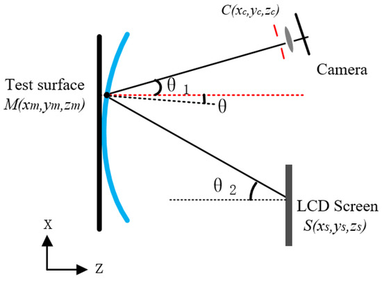
Figure 1.
Schematic of PMD test system.
The surface slope equations are shown in Equation (1) by Su et al. [5] in 2010.
where are the coordinates of the pinhole camera. are the coordinates of the sampling point on the test surface. are the coordinates of the illuminated pixel on the LCD screen that can be calculated by the phase shifting method.
is the distance between the test surface and the screen and is the distance between the test surface and the camera. Then, substituting these coordinates into Equation (1) can obtain the slope data, and the surface is reconstructed with slope-based integration algorithms.
2.2. The Principle of RBF Integration Method
The weighted combination of analytical derivatives of the RBF integration method is used to represent the test surface in Equation (2), where is the Wendland [21] radial basis function and can be written as Equation (3).
In Equation (3), is a scaling factor that can be adjusted to make the reconstruction have high quality [22]. The relation between the analytical derivatives of and the measured slope values and based on PMD can be established in Equation (4).
After expressing Equation (4) as a matrix form and using the least squares method to obtain and , the surface W can be obtained by taking the resulting coefficients and back into Equation (2). The Wendland radial basis function has a high-order continuity property to meet the integrability condition, and Hermite interpolation is applicable to discrete data [23], which makes it feasible to deal with the quadrilateral geometry issue.
2.3. Ray Tracing Model
In the process of the light from the LCD screen entering the camera through the pinhole after being reflected from the test surface, the coordinates of the reflected points on the unit under test (UUT) in the PMD system can be obtained by using the iterative method in a ray tracing model [24,25,26], as shown in Figure 2. Firstly, we use the coordinate of a certain screen pixel and the direction cosine of the light emitted from this pixel as the initial data, where are defined as directional cosines of this ray around the , respectively. Then, the coordinate of intersection point of the light on the tangent plane of the component coordinate system is calculated in Equation (5):
where is the distance in the -direction between the tangent plane and , denotes the distance from the starting point of the ray to , and take the point as the first approximate solution of the intersection point to be solved. Consequently, a line starting from the point of which is parallel to the optical axis is intersected with the surface of the component at the point of , and the tangent plane of the element formed through point is expressed as Equation (6). The coordinates of are the same as those of , and the z coordinate is calculated by .
where, , and are the normal components at point in the x, y, and z directions, respectively.
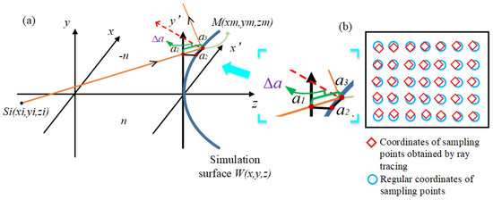
Figure 2.
(a) Ray tracing; (b) The difference between the sampling point coordinates of regular rectangular grids and the coordinates of sampling points obtained by ray tracing.
Next, the tangent plane passing through the point of intersects with the ray at the point of , which is used as a new approximate solution. Let which is the distance between them, so we can obtain the following relationship.
Equation (8) is substituted into Equation (6) to obtain the following Equation (9), then we can obtain the at last.
The above steps are repeated until is smaller than a pre-setting threshold, and will be very close to the coordinate of the reflected point of the surface. Therefore, can be treated as the coordinate of reflection point on UUT.
From the previous derivation, we can obtain the actual coordinates of the sampled points exactly by ray tracing, and there is a difference between the sampling point coordinates of regular rectangular grids and the coordinates of sampling points obtained by ray tracing, as shown in Figure 2b. The ray-traced sampling points are used in the integration process as in Equation (4) in both simulation and experiment.
3. Numerical Simulations and Experiments
3.1. Numerical Simulations
In off-axis PMD configuration, the measured surface is not perpendicular to the optical axis of the camera lens, as shown in Figure 1. The experimental deformed patterns of three typical surfaces under test, including the convex, the concave, and the flat, are separately recorded by the camera as shown in Figure 3a–c when a straight fringe pattern is displayed on the screen. In order to verify the method in Section 2 mentioned above, the three cases are simulated, where the normal of the measured surface is not parallel to the optical axis of the camera lens, a convex sphere, and a concave sphere, the radius of curvature and diameter of which are 300 mm and 120 mm, respectively; additionally a free-form surface with the area of 120 mm × 120 mm and sampling points of 120 × 120. Their fringe patterns acquired by the camera and coordinate points obtained by using the iterative method in the tracing model are shown in Figure 3a–f, respectively.
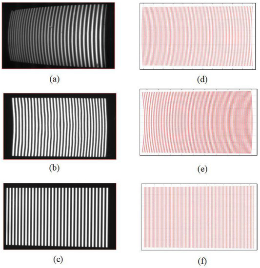
Figure 3.
Experiment patterns and ray tracing patterns. (a–c) Fringe patterns experimentally acquired by the configuration in Figure 1 for a convex, a concave, and a free-form surface, respectively; (d–f) coordinate points obtained by ray tracing with the configuration in Figure 1 for a convex, a concave, and a free-form surface, respectively.
The simulation demonstrates that these quadrilateral geometries in Figure 3a–c acquired by the CCD camera are similar to the results of ray tracing in Figure 3d–f. The keystone distortion and the shape of patterns agree with the experiments. For the three elements, their coordinates and the slope of each sampling point are obtained by ray tracing at the angle of 8°, 11°, 14°, 17°, and 20°, respectively. The simulated surface is then reconstructed using the improved Southwell algorithm and the RBF interpolation algorithm, respectively. Random noise with a mean value of 0.017 mm [27] is added to the screen coordinates. The reconstructed residual errors are differences between the reconstructed surface and the ground truth, the RMS and PV (Peak Value) values of the residual errors for the two algorithms at different angles are shown in the Appendix of Table A1 and Table A2, and the RMS values of the residual error of the two methods are multiplied by 106 and taken logarithmically and plotted as Figure 4 and Figure 5.
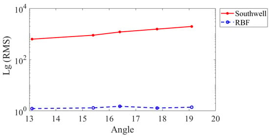
Figure 4.
RMS of residual error a convex sphere using Southwell and RBF with different angles.
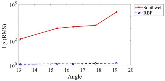
Figure 5.
RMS of residual error of a concave sphere using Southwell and RBF with different angles.
For both convex and concave spheres, the RMS value of the reconstruction residual error of the RBF interpolation algorithm is approximately 10−6 mm, while the PV value is approximately 10−5 mm. In contrast, the RMS value of the reconstruction residual error of the improved Southwell algorithm is approximately 10−4 mm, while the PV value is approximately 10−3 mm. The simulation results indicate that the RBF interpolation algorithm offers nearly one order of magnitude better reconstruction accuracy for this quadrilateral geometry, and the keystone distortion hardly impacts the accuracy of reconstruction. A surface function defined as Equation (11) which is more frequently used [10,17], is combined with a plane to represent a common free-form surface to verify the advantages of RBF, and the height distribution of a simulated free-form surface seen in Figure 6.
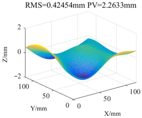
Figure 6.
Height distribution of a simulated free-form surface.
The RMS values of the residual error of the two methods are multiplied by 104 and taken logarithmically and plotted, as shown in Figure 7. The reconstruction results of the RBF interpolation algorithm are better than those of the improved Southwell algorithm for the free-form surface at different angles, and the RMS values and PV values can be seen in the Appendix of Table A3. Therefore, the simulations above using ray tracing verify that the RBF interpolation algorithm is more practical for an off-axis PMD system.
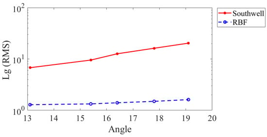
Figure 7.
RMS of residual error of a free-form surface using Southwell and RBF with different angles.
3.2. Experimental Results
An investigation of off-axis PMD is carried out as well, and Figure 8 shows the experimental setup, which includes a CCD camera with an external diaphragm, a flat surface to be measured, and a screen to display sinusoidal fringe patterns with a period of 21 pixels. The optical axis of the camera lens is approximately 13.1°, 15.4°, 16.4°, 17.8°, and 19.1° away from the normal of the surface being measured. The size of the test flat glass element in diameter is 200 mm, and the measured area of it is a square with side lengths of roughly 142 mm. Based on the setup in Figure 8, the distorted fringe pattern captured by the CCD camera at different angles, as shown in Figure 9, and the calculated area, which is boxed by the dotted red lines, includes 355 × 355 pixels.
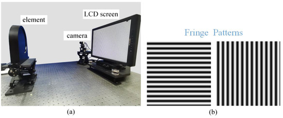
Figure 8.
Experimental setup. (a) Experimental components and general placement; (b) The sinusoidal fringe patterns to be displayed on a screen.
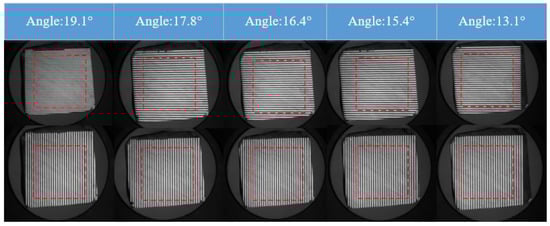
Figure 9.
Distorted fringe pattern captured by the camera at different angles in the x and y direction, respectively.
Decreasing the sample points can reduce computation time and save computer memory because the flat primarily contains a large amount of low-frequency information, as shown in Figure 9. As a consequence, the data points are sampled to create a 121 × 121-pixel matrix. The camera records the phase-shifted sinusoidal fringe patterns in two directions. Their deformation depends on the surface figure, the posture of the camera, and the surface shape of the element inducing. Next, a sixteen-step phase shifting method is used to determine the correspondence between the camera pixel and the screen pixel, Starting with a surface assumption, are determined with ray tracing as described in Section 2.3. Then, the slope calculated from Equation (1) is integrated. The integrated surface is put back to update the sampling point by ray tracing to iteratively calculate the slope. Finally, the improved Southwell method and RBF interpolation algorithm are applied to reconstruct the surface with the slopes in the x and y directions. Then, the tilt of the acquired surface shape is removed using the Chebyshev polynomial fitting algorithm. The experimental result is given in Figure 10 for the maximum angle of 19.1°, and experimental results for other angles are given in the Appendix from Figure A1, Figure A2, Figure A3 and Figure A4. Meanwhile, the RMS values of the residual error of the two methods are plotted as Figure 11.
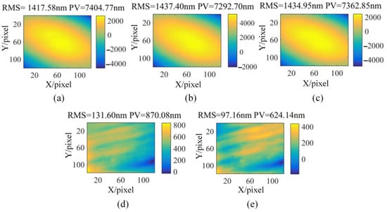
Figure 10.
The experimental results at the angle of 19.1°. (a) The result of interferometer without the Chebyshev’s first three terms; (b) Reconstruct wavefront without the Chebyshev’s first three terms using Southwell; (c) Reconstruct wavefront without the Chebyshev’s first three terms using RBF; (d) is the difference between (a,b); (e) is the difference between (a,c).
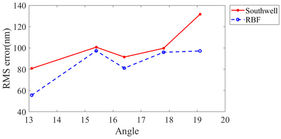
Figure 11.
The RMS of two methods at five different angles.
Taking Figure 10 as an example, the first three terms of the Chebyshev polynomial are removed from the result of the interferometer, as shown in Figure 10a. Figure 10b,c are the reconstructed surface shape without the first three terms using the Southwell and RBF, respectively. Figure 10d is the surface shape difference between the interferometer result and the reconstruction result of Southwell, and Figure 10e is the surface shape difference between the interferometer result and the reconstruction result of RBF. For the five different angles, by comparing with the result of the interferometer, it shows that all of the RMS obtained by the RBF interpolation algorithm are smaller than those of the improved Southwell algorithm. Noticeably, the RMS of the improved Southwell algorithm reconstruction residual error is 131.6 nm, while the RMS of RBF is 97.16 nm when the angle is the maximum of 19.1° in our experiment.
In addition, we conducted repeatability experiments for a flat element, and the results of our repeatability experiments are depicted in Figure 12; the numbers 1, 2, and 3 in the label in the figure’s upper right corner indicate that there are three experiments at five angles. The results verify that the reconstruction results of the RBF interpolation algorithm have higher accuracy.
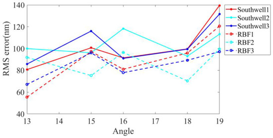
Figure 12.
The RMS of repeatability experiments with two methods at different angles.
3.3. KDP Crystal Pre-Surface Testing Based on Off-Axis PMD
Due to the parasitic reflection in the detection of transparent optical elements, the structured light coding pattern projected by the screen is reflected by both the front and rear surfaces of the transparent optical elements. The CCD camera captures the fringe pattern on the front and rear surfaces superimposed on each other, and the fringe pattern no longer satisfies the sinusoidal distribution, so the traditional phase shifting method will fail to solve for the correct screen pixel coordinates. In order to better separate the front and rear surface information of KDP crystals, this paper adopts a binary pattern method based on off-axis PMD [8]. After obtaining the coordinates of the screen reflected through the front surface using the binary pattern method, the slope can be calculated using Equation (1). The measurement size is a 72 mm × 72 mm square containing 400 × 400 pixels, which are sampled and transformed into a 100 × 100 matrix.
The measurement results are shown in Figure 13. Figure 13d shows the RMS value of 84.21 nm for the difference between the first four terms removed after reconstructing the front surface of the KDP crystal using Southwell and the first four terms removed by the interferometer, while Figure 3e shows only the RMS value of 47.76 nm for the difference between the first four terms removed after reconstructing the front surface of the KDP crystal using RBF and the first four terms removed by the interferometer.
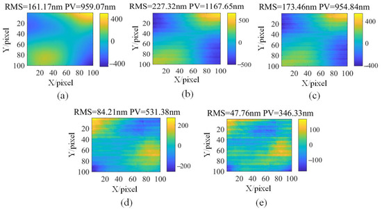
Figure 13.
The results of KDP crystal front surface reconstruction. (a) The result of interferometer without the Chebyshev’s first four terms; (b) reconstruct wavefront without the Chebyshev’s first four terms using Southwell; (c) reconstruct wavefront without the Chebyshev’s first four terms using RBF; (d) is the difference between (a,b); (e) is the difference between (a,c).
4. Discussion and Conclusions
In the off-axis PMD, the sampling points are no longer equally spaced on a regular rectangular grid due to the tilted camera, and a distorted quadrilateral geometry is generated, making it difficult to reconstruct a wavefront with higher accuracy. In this paper, the quadrilateral geometry under this perspective effect is simulated at different angles by performing ray tracing for different surfaces to acquire the reflection point coordinates. Numerical simulation demonstrates that for the reconstruction of all three different surfaces, the RBF interpolation algorithm works better than the improved Southwell algorithm, which can reach a higher accuracy than the traditional Southwell. To further verify the reconstruction capability of the RBF interpolation algorithm for this quadrilateral geometry, experimentally, the camera is tilted at different angles, and the repeatability experiments also are implemented three times at five different angles. All the experimental results show that RBF is able to reconstruct the surface shape even the camera is tilted at a large angle and with about tens of nm RMS higher reconstruction accuracy than the Southwell algorithm. Finally, the front surface shape of the KDP crystal is reconstructed using the RBF interpolation algorithm, and the reconstruction accuracy is higher compared with the reconstruction result of the improved Southwell algorithm. However, some issues, such as lens distortion, system configuration and alignments, etc., need to be considered if a significant improvement in accuracy for the RBF is experimentally pursued.
Author Contributions
Conceptualization, H.W. and D.L.; methodology, H.W. and D.L.; software, H.W., D.L., X.Z., R.G. and W.Z.; data curation, H.W., D.L. and X.Z.; writing—original draft preparation, H.W.; writing—review and editing, D.L., X.Z., R.G. and W.Z. All authors have read and agreed to the published version of the manuscript.
Funding
This research is funded by the National Natural Science Foundation of China (grant numbers: U20A20215 and 61875142) and Sichuan University (grant number: 2020SCUNG205).
Institutional Review Board Statement
Not applicable.
Informed Consent Statement
Not applicable.
Data Availability Statement
Not applicable.
Acknowledgments
We would like to thank Lei Huang, who kindly helped us with the RBF algorithm.
Conflicts of Interest
The authors declare no conflict of interest.
Appendix A

Table A1.
Simulation results of a convex sphere at different angles for two methods. Unit: mm.
Table A1.
Simulation results of a convex sphere at different angles for two methods. Unit: mm.
| Methods/Angles | 8° | 11° | 14° | 17° | 20° |
|---|---|---|---|---|---|
| RMS | RMS | RMS | RMS | RMS | |
| Southwell | 6.2796 × 10⁻⁴ | 8.9421 × 10⁻⁴ | 1.1956 × 10⁻³ | 1.5453 × 10⁻³ | 1.9634 × 10⁻³ |
| RBF | 1.2303 × 10⁻⁶ | 1.3114 × 10⁻⁶ | 1.5102 × 10⁻⁶ | 1.2916 × 10⁻⁶ | 1.392 × 10⁻⁶ |
| PV | PV | PV | PV | PV | |
| Southwell | 2.751 × 10⁻³ | 3.8075 × 10⁻³ | 5.0341 × 10⁻³ | 6.4804 × 10⁻³ | 8.2391 × 10⁻³ |
| RBF | 2.1682 × 10⁻⁵ | 2.3822 × 10⁻⁵ | 2.3886 × 10⁻⁵ | 2.3638 × 10⁻⁵ | 2.9017 × 10⁻⁵ |
Table A2.
Simulation results of a convex sphere at different angles for two methods. Unit: mm.
Table A2.
Simulation results of a convex sphere at different angles for two methods. Unit: mm.
| Methods/Angles | 8° | 11° | 14° | 17° | 20° |
|---|---|---|---|---|---|
| RMS | RMS | RMS | RMS | RMS | |
| Southwell | 1.3774 × 10⁻⁴ | 1.0486 × 10⁻³ | 1.3991 × 10⁻³ | 1.8042 × 10⁻³ | 2.2842 × 10⁻³ |
| RBF | 1.1581 × 10⁻⁶ | 1.3097 × 10⁻⁶ | 1.2639 × 10⁻⁶ | 1.4003 × 10⁻⁶ | 1.4558 × 10⁻⁶ |
| PV | PV | PV | PV | PV | |
| Southwell | 5.9239 × 10⁻³ | 8.4416 × 10⁻³ | 1.1278 × 10⁻² | 1.4551 × 10⁻² | 1.8427 × 10⁻² |
| RBF | 1.8636 × 10⁻⁵ | 2.4124 × 10⁻⁵ | 2.5955 × 10⁻⁵ | 2.4068 × 10⁻⁵ | 2.9257 × 10⁻⁵ |
Table A3.
Simulation results of a simulated free-form surface at different angles for two methods. Unit: mm.
Table A3.
Simulation results of a simulated free-form surface at different angles for two methods. Unit: mm.
| Methods/Angles | 8° | 11° | 14° | 17° | 20° |
|---|---|---|---|---|---|
| RMS | RMS | RMS | RMS | RMS | |
| Southwell | 6.7733 × 10⁻⁴ | 9.5299 × 10⁻⁴ | 1.2637 × 10⁻³ | 1.6199 × 10⁻³ | 2.0353 × 10⁻³ |
| RBF | 1.2881 × 10⁻⁴ | 1.3348 × 10⁻⁴ | 1.4040 × 10⁻⁴ | 1.4979 × 10⁻⁴ | 1.6185 × 10⁻⁴ |
| PV | PV | PV | PV | PV | |
| Southwell | 4.8661 × 10⁻³ | 7.0352 × 10⁻³ | 9.4538 × 10⁻³ | 1.2206 × 10⁻² | 1.5405 × 10⁻² |
| RBF | 8.8785 × 10⁻⁴ | 9.0465 × 10⁻⁴ | 9.2675 × 10⁻⁴ | 9.4235 × 10⁻⁴ | 9.4867 × 10⁻⁴ |

Figure A1.
The experimental results at the angle of 13.1°. (a) The result of interferometer without the Chebyshev’s first three terms; (b) reconstruct wavefront without the Chebyshev’s first three terms using Southwell; (c) reconstruct wavefront without the Chebyshev’s first three terms using RBF; (d) is the difference between (a,b); (e) is the difference between (a,c).


Figure A2.
The experimental results at the angle of 15.4°. (a) The result of interferometer without the Chebyshev’s first three terms; (b) reconstruct wavefront without the Chebyshev’s first three terms using Southwell; (c) reconstruct wavefront without the Chebyshev’s first three terms using RBF; (d) is the difference between (a,b); (e) is the difference between (a,c).


Figure A3.
The experimental results at the angle of 16.4°. (a) The result of interferometer without the Chebyshev’s first three terms; (b) reconstruct wavefront without the Chebyshev’s first three terms using Southwell; (c) reconstruct wavefront without the Chebyshev’s first three terms using RBF; (d) is the difference between (a,b); (e) is the difference between (a,c).


Figure A4.
The experimental results at the angle of 17.8°. (a) The result of interferometer without the Chebyshev’s first three terms; (b) reconstruct wavefront without the Chebyshev’s first three terms using Southwell; (c) reconstruct wavefront without the Chebyshev’s first three terms using RBF; (d) is the difference between (a,b); (e) is the difference between (a,c).

References
- Knauer, M.C.; Kaminski, J.; Häusler, G. Phase measuring deflectometry: A new approach to measure specular free-form surfaces. In Optical Metrology in Production Engineering; SPIE: Bellingham, DC, USA, 2004; pp. 366–376. [Google Scholar]
- Jin, C.; Li, D.; Kewei, E.; Li, M.; Chen, P.; Wang, R.; Xiong, Z. Phase extraction based on iterative algorithm using five-frame crossed fringes in phase measuring deflectometry. Opt. Lasers Eng. 2018, 105, 93–100. [Google Scholar] [CrossRef]
- Huang, L.; Idir, M.; Zuo, C.; Asundi, A. Review of phase measuring deflectometry. Opt. Lasers Eng. 2018, 107, 247–257. [Google Scholar] [CrossRef]
- Burke, J.; Pak, A.; Hfer, S.; Ziebarth, M.; Roschani, M.; Beyerer, J. Deflectometry for specular surfaces: An overview. arXiv 2022, arXiv:2204.11592. [Google Scholar]
- Su, P.; Parks, R.E.; Wang, L.R.; Angel, R.P.; Burge, J.H. Software configurable optical test system: A computerized reverse Hartmann test. Appl. Opt. 2010, 49, 4404–4412. [Google Scholar] [CrossRef]
- Su, P.; Khreishi, M.; Su, T.Q. Aspheric and freeform surfaces metrology with software configurable optical test system: Acomputerized reverse Hartmann test. Opt. Eng. 2014, 53, 031305. [Google Scholar] [CrossRef]
- Xu, Y.; Gao, F.; Jiang, X. A brief review of the technological advancements of phase measuring deflectometry. PhotoniX 2020, 1, 1–10. [Google Scholar] [CrossRef]
- Wang, R.; Li, D.; Xu, K.; Zhang, X.; Luo, P. Parasitic reflection elimination using binary pattern in phase measuring deflectometry. Opt. Commun. 2019, 451, 67–73. [Google Scholar] [CrossRef]
- Huang, R.; Su, P.; Horne, T.; Brusa, G.; Burge, J.H. Optical metrology of large deformable aspherical mirror using software configurable optical test system. Opt. Eng. 2014, 50, 085106. [Google Scholar] [CrossRef]
- Huang, L.; Asundi, A.K. Framework for gradient integration by combining radial basis functions method and least-squares method. Appl. Opt. 2013, 52, 6016–6021. [Google Scholar] [CrossRef]
- Freischlad, K.R.; Koliopoulos, C.L. Modal estimation of a wave front from difference measurements using the discrete Fourier transform. J. Opt. Soc. Am. A 1986, 3, 1852–1861. [Google Scholar] [CrossRef]
- Dai, G.M. Modal wave-front reconstruction with Zernike polynomials and Karhunen–Loève functions. J. Opt. Soc. Am. A 1996, 13, 1218–1225. [Google Scholar] [CrossRef]
- Fried, D.L. Least-square fitting a wave-front distortion estimate to an array of phase-difference measurements. Opt. Soc. Am. 1977, 67, 370–375. [Google Scholar] [CrossRef]
- Southwell, W.H. Wave-front estimation from wave-front slope measurements. J. Opt. Soc. Am. 1980, 70, 998–1006. [Google Scholar] [CrossRef]
- Li, M.; Li, D.; Jin, C.; Kewei, E.; Yuan, X.; Xiong, Z.; Wang, Q. Improved zonal integration method for high accurate surface reconstruction in quantitative deflectometry. Appl. Opt. 2017, 56, F144–F151. [Google Scholar]
- Ettl, S.; Kaminski, J.; Knauer, M.C.; Häusler, G. Shape reconstruction from gradient data. Appl. Opt. 2008, 47, 2091–2097. [Google Scholar] [CrossRef]
- Huang, L.; Idir, M.C.; Chao, Z.; Kaznatcheev, K.; Zhou, L.; Asundi, A. Comparison of two-dimensional integration methods for shape reconstruction from gradient data. Opt. Laser Eng. 2015, 64, 1–11. [Google Scholar] [CrossRef]
- Ren, H.; Gao, F.; Jiang, X. Improvement of high-order least-squares integration method for stereo deflectometry. Appl. Opt. 2015, 54, 10249–10255. [Google Scholar] [CrossRef]
- Ren, H.; Gao, F.; Jiang, X. Least-squares method for data reconstruction from gradient data in deflectometry. Appl. Opt. 2016, 55, 6052–6059. [Google Scholar] [CrossRef]
- Huang, L.; Xue, J.; Gao, B.; Zuo, C.; Idir, M. Zonal wavefront reconstruction in quadrilateral geometry for phase measuring deflectometry. Appl. Opt. 2017, 56, 5139. [Google Scholar] [CrossRef]
- Wendland, H. Piecewise polynomial, positive definite and compactly supported radial functions of minimal degree. Adv. Comput. Math. 1995, 4, 389–396. [Google Scholar] [CrossRef]
- Lowitzsch, S. Matrix-valued radial basis functions: Stability estimates and applications. Adv. Comput. Math. 2005, 23, 299–315. [Google Scholar] [CrossRef]
- Lowitzsch, S.; Kaminski, J.; Knauer, M.C.; Häusler, G.; Knauer, M.C. Vision and modeling of specular surfaces. Vis. Model. Vis. 2005, 479–486. [Google Scholar]
- Li, L.; An, L.S. Theory and Application of Computer Aided Optical Design; National Defence Industry Press: Beijing, China, 2002; pp. 40–43. [Google Scholar]
- Díaz-Uribe, R.; Campos-García, M. Null-screen testing of fast convex aspheric surfaces. Appl. Opt. 2000, 39, 2670–2677. [Google Scholar] [CrossRef] [PubMed]
- Campos-García, M.; Bolado-Gómez, R.; Díaz-Uribe, R. Testing fast aspheric concave surfaces with a cylindrical null screen. Appl. Opt. 2008, 47, 849–859. [Google Scholar] [CrossRef] [PubMed]
- Huang, L.; Xue, J.; Gao, B.; McPherson, C.; Beverage, J.; Idir, M. Modal phase measuring deflectometry. Opt. Express 2016, 24, 24649–24664. [Google Scholar] [CrossRef] [PubMed]


Disclaimer/Publisher’s Note: The statements, opinions and data contained in all publications are solely those of the individual author(s) and contributor(s) and not of MDPI and/or the editor(s). MDPI and/or the editor(s) disclaim responsibility for any injury to people or property resulting from any ideas, methods, instructions or products referred to in the content. |
© 2023 by the authors. Licensee MDPI, Basel, Switzerland. This article is an open access article distributed under the terms and conditions of the Creative Commons Attribution (CC BY) license (https://creativecommons.org/licenses/by/4.0/).