Crowd Density Level Estimation and Anomaly Detection Using Multicolumn Multistage Bilinear Convolution Attention Network (MCMS-BCNN-Attention)

Abstract

The detection of crowd density levels and anomalies is a hot topic in video surveillance. Especially in human-centric action and activity-based movements. In some respects, the density level variation is considered an anomaly in the event. Crowd behaviour identification relies on a computer-vision-based approach and basically deals with spatial information of foreground video information. In this work, we focused on a deep-learning-based attention-oriented classification system for identifying several basic movements in public places, especially, human flock movement, sudden motion changes and panic events in several indoor and outdoor places. The important spatial features were extracted from a bilinear CNN and a multicolumn multistage CNN with preprocessed morphological video frames from videos. Finally, the abnormal and crowd density estimation was distinguished by using an attention feature combined with a multilayer CNN feature by modifying the fully connected layer for several categories (binary and multiclass). We validate the proposed method on several video surveillance datasets including PETS2009, UMN and UCSD. The proposed method achieved an accuracy of 98.62, 98.95, 96.97, 99.10 and 98.38 on the UCSD Ped1, UCSD Ped2, PETS2009, UMN Plaza1 and UMN Plaza2 datasets, respectively, with the different pretrained models. We compared the performance between recent modern approaches and the proposed method (MCMS-BCNN-Attention) and achieved the highest accuracy. The anomaly detection performance on the UMN and PETS2009 datasets was compared with that of a state-of-the-art method and achieved the best AUC results as 0.9953 and 1.00 for both scenarios, respectively, with a binary classification.

1. Introduction

One of the key security issues during public events is how to accurately determine activity when people are moving and congregating. The congestion levels and anomaly detection are also extremely difficult tasks in video surveillance. With the expansion of human society activities, surveillance in recent years has become a very important and difficult task. In this work, we mainly focused on several events in indoor and outdoor environments while some events occurred in low light conditions and had shadows with large occlusions. An efficient crowd behaviour analysis is required to identify the abnormality of a crowd gathering and understand its behaviour by analysing video information in public surveillance videos. The analysed information is very useful to use for crowd management in public spaces based on predefined behaviours.

However, in recent years, the technology of surveillance equipment has been significantly advanced in order to improve the quality of the obtained spatial information. Event spot analysis is still a difficult task due to the long viewing distance and the low-resolution quality of surveillance videos. The current approach to testing videos with a resolution of almost 299 × 299 pixels with high occlusion allows a relatively low-quality video. In principle, there are surveillance methods available in real time, leaving the analysis for later in case of a special investigation. However, both methods require a special interaction with a person to analyse the video, which can lead to visual fatigue and psychological weakness. Thus, the interaction with instances and a quick attention to unexpected situations, such as an abnormal event or a cluster of abnormal people, have a great impact on the task of video surveillance.

Technically, an anomaly can be described as an unusual movement of a person, a cluster or a sudden convergence/divergence in a certain area of interest. In addition, crowd density level analysis measures the anomaly of traffic forecasting in surveillance video. The crowd analysis is mainly divided into several subsessions such as density, abnormal activity, crime scene, crowd counting, event understanding and many more. The group activity detection and event understanding need highly improved spatial–temporal model information to understand behaviours. The basic methods of all the crowd behaviour understanding are based on conventional spatial–temporal features such as handcrafted and convolution kernel features. Figure 1 shows the basic workflow of our proposed approach to understanding crowd behaviour in the public environment. The main contribution of the model provides an efficient deep learning feature extraction by modifying the existing conventional model to understand crowd congestion levels in public areas. The manually annotated congestion levels of information are described in Table 1 briefly. The congestion level in the scene is highly involved in understanding abnormal activity in the crowd.

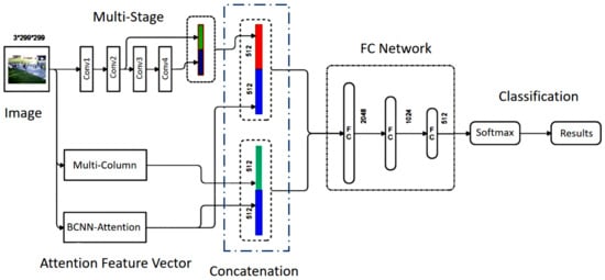
Figure 1. The network architecture of the proposed model.

Table 1. Bilinear attention network’s parameter information (densenet121).

Input	3 × 299 × 299
Layer	Output	Filter Size	Neurons
Convolution	112 × 112	7 × 7	3 × 64
Pooling	56 × 56	3 × 3	64
Dense Block	56 × 56	(1 × 1, 3 × 3) 6	64 × 256
Transition	(56 × 56, 28 × 28)	(1 × 1, 2 × 2)	256 × 128
Dense Block	28 × 28	(1 × 1, 3 × 3) 12	128 × 512
Transition	(28 × 28, 14 × 14)	(1 × 1, 2 × 2)	512 × 256
Dense Block	14 × 14	(1 × 1, 3 × 3) 24	256 × 1024
Transition	(14 × 14, 7 × 7)	(1 × 1, 2 × 2)	1024 × 512
Dense Block	7 × 7	(1 × 1, 3 × 3) 16	512 × 1024
Dropout (0.5)
Attention	1024
FC	512

In this paper, we introduce a model to extract spatial information to detect basic activity and crowd density from attention-based feature classification with a multiclass CNN. There are several ways to understand the crowd density in a video sequence. In our approach, a sequence was divided into five congestion levels and tested with publicly available datasets described in the experiments and results section. The congestion levels were categorized from low to high as very low (VL), low (L), medium (M), high (H) and very high (VH). The proposed model was developed by fine-tuning of a densenet121 [1] and Efficientnetv2 [2] network and a multicolumn [3] CNN architecture to extract multichannel features from a single image instance.

The bilinear CNN was based on the simultaneous extraction of different object features (different kernel size) from the same instance and at the same time, a multicolumn CNN was utilized to extract different filters to extract dense features from the same image. The parallel features were gathered before the fully connected layer by combining with the outer products of matrices. Dense object features were extracted simultaneously by using various image convolution filters to create a density map by combining each channel. The final outcome was trained with a fusion network followed by a fully connected layer to classify the final categories. The total training loss parameters were calculated during the training by summing each network’s partial loss. The loss function could be optimized with the same gradient descent optimization as backpropagation in training neural networks. The different-kernel-size filters could effectively extract multiple features with a bilinear attention network to improve the foreground and background information of the scene features at the same time. The conventional multistage- and multicolumn-generated features missed more imported features in a given image than the combined attention features (proposed model). Therefore, a significant classification improvement was achieved, as discussed in the results analysis section. Early stopping was used in the model training strategy to achieve better outcomes, and the fused features experienced faster training convergence than traditional techniques.

Contribution of the Work

The multistage, multicolumn layers improved spatial information along the attention features. In this approach, we introduced several modifications to improve the deep features from spatial information. The main contribution process of building the novel bilinear attention feature vector and fusion network process is explained as follows: The proposed model introduced three main parallel feature extraction methods to improve features at different levels. Mainly, bilinear CNN pooling networks extract different features at different depth levels. Therefore, bilinear feature extraction models extract richer features (deep features) than normal convolution networks. Our approach used a dual-channel feature extraction model (transfer learning) based on densenet121 and Efficientnetv2 for generating the bilinear pooling matrix in a given image. The generate bilinear feature matrix was used to calculate the attention score matrix of each point by multiplying it with the activation weight vector. Finally, we obtained the attention feature vector by aggregating all column elements together to generate a bilinear attention feature vector. Second, the single-image multicolumn network was modified with a convolution layer and a fully connected layer to generate a feature vector instead of a feature map. The generated density feature vector and subsampled multistage convolution feature vector were parallelly concatenated with the bilinear attention feature vector. Finally, the two streams flattened the feature vectors, which were fed into a fully connected fusion network with a softmax classification.

Experiments were conducted at different density levels using benchmarks, including PETS 2009, UMN and UCSD. The training and validation outcomes performed best, as mentioned in the results section, and were also compared with state-of-the-art algorithms.

2. Related Works

Crowd anomaly or density level detection plays a key role in monitoring and surveillance of crowded places. It prevents mishaps and crime in a congested environment. The main problem for anomaly classification in crowded areas is using feature sets and techniques that can be replicated in every crowded scenario [4]. Anomaly detection in a crowded environment is classified as trajectory-based or feature-based [5]. In a trajectory-based detection system, the trajectories of moving crowds are obtained using target-tracking models. After acquisition, these trajectories are compared with normal trajectories gained by applying machine learning to normal situations to gain potential knowledge. After this process, anomalies are detected [6]. Ref. [7] presented a real-time anomaly recognition in average-density crowd videos using trajectory-level behaviour training. The proposed algorithm combined a particle filter online-tracking model and RVO (reciprocal velocity obstacle), a nonlinear pedestrian motion model, to estimate the dense crowd environment’s motion trajectory. The proposed model used a Bayesian learning technique to estimate the trajectory of each person in videos. The PETS2016 ARENA dataset was used for the experimental results evaluation. Ref. [8] proposed an online tool to detect the trajectory points in real time and detect the outliers as normal or abnormal. The proposed method used the video frame’s temporal window and the threshold value of a trajectory to classify it as normal or abnormal. Ref. [9] used the short local trajectory (SLT) for the detection of abnormal objects in a video. The proposed scheme used HMM (hidden Markov model) for acquiring the normal trajectory patterns. Ref. [10] used the histogram method of optical flow known as PT-HOF to detect an abnormality. Moreover, the scheme used spatial features and temporal information to form PT-HOF. However, the trajectory-based anomaly detection methods were only appropriate for small-level, low-density scenes. The increase in crowd size forces the trajectory to overlap, which decreases the accuracy and preciseness of anomaly detection algorithms. On the other hand, the feature-based approaches split the video into different regions of interest (ROI). Then, the features are extracted from different ROIs to learn activity patterns [11]. Ref. [12] proposed a spatial–temporal texture method also known as STT for feature extraction from video scenes. First, spatiotemporal volumes (STV) were constructed from a raw video. For further processing, a slice of STV or STT was extracted to find hidden patterns. Then, the Shannon entropy of each STT was calculated to estimate information available in each frame. The STT with a higher entropy was chosen as the objective STT for people behaviour evaluation. Then, a grey-level co-occurrence matrix (GLCM) was used to extract features from the targeted STT. These extracted features were applied to different machine learning algorithms, including SVM, KNN, naïve Bayes and random forest, for abnormality detection. Ref. [13] proposed a novel approach for anomaly detection built on a DNN. The model used optical flow maps and 3D gradient for anomaly recognition. The MGFC-AAE network involved two DNNs: an encoder network and a discriminator. During the training phase, the gradient value and optical flow patches of usual scenes were separated. For testing a given region, MGFC-AAE was used for the latent representations of the patch gradient and optical flow. Then, an energy-based technique was used to calculate the motion anomaly score and its appearance. Ref. [14] proposed a dynamic-based and deep dynamic-based network for object detection and the histogram variance of optical flow angle (HVO) with motion energy to discover unusual motion patterns. It used spatial and temporal information for tracking strange objects. Ref. [15] proposed an attention-enhanced graph convolutional LSTM network (AGC-LSTM) to detect individual action using skeleton data. The suggested scheme was able to capture the discriminative spatiotemporal features effectively. Ref. [16] proposed a descriptor that analyse the crowd dynamics in real time by observing the crowd texture changes. GLCM features were used for temporal summaries. The authors also proposed the interframe uniformity (IFU), which explained the change in violent behaviour compared to normal crowd behaviour changes. The proposed method used the Haralick texture features obtained from each frame of the sequences and described the involvement of these features in crowd dynamics. It also emphasized that violent behaviour usually had a less uniform rate of changes over time than normal crowd behaviour. Ref. [17] used an autoencoder to detect anomalies in crowded videos. After a training process, the autoencoder identified the complicated distribution of the normal dynamics of behaviour change. It used state-of-the-art hand-crafted HOG and HOF motion features models with enhanced trajectory features as an autoencoder input. The autoencoder learned the regular motion signatures by using a fully connected neural network. As these motion features could not be ideal for anomaly detection, the model learned the motion features and trained the encoder using an end-to-end learning version of a fully connected CNN during training. The learned model was analysed by visualizing the consistency in frames also predicting a normal past and future frame utilizing a single image. Ref. [18] proposed a convolutional LSTM built on an autoencoder-based approach for anomaly detection in videos. With the help of a CNN, the authors characterized each frame’s content in the video, and ConvLSTM was used to characterize the motion information. Moreover, ConvLSTM preserved the spatial information, which helped the reconstruction of frames. Ref. [19] proposed MemAE, a memory-augmented autoencoder for anomaly detection. The model consisted of three units: an encoder, a decoder and a memory unit. Ref. [20] used a CNN model for feature extraction and context analysis from surveillance videos. Then, it used a denoising autoencoder to deliver precise surveillance anomaly detection. To construct the background segmentation features, it used a panoptic feature pyramid network (PFPN). The PFPN model was also used to solve unified tasks on amorphous background regions such as rivers, walls, etc. The proposed model used the joint detection and embedding (JDE) model for pedestrian detection and tracking features. Ref. [21] suggested an unsupervised deep learning framework to analyse the anomalies in crowded videos. The handcrafted features included energy features, low-level visual features and a motion map, and these features were used for anomaly detection in a video. The proposed scheme consisted of three stages. Firstly, three CDBNs were used to learn the midlevel features from crowd data. Secondly, these midlevel features were merged using a fusion scheme to form a deep high-level representation. Finally, a one-class support vector machine (SVM) was used to learn from the deep representation. Based on this learning, the SVM detected any abnormal data existing in crowd videos. Ref. [22] used a deep cascade autoencoder (CDA) to detect any abnormal event in surveillance videos. The moment information was captured by a motion descriptor, namely a multiframe descriptor (MHOFO). Then, these features extracted by a descriptor were fed to the CDA network for the training process. After training, the abnormal events were distinguished from the normal ones using the error rate of the CDA. Ref. [23] proposed a novel approach named aggregation of ensembles for abnormality recognition in surveillance videos. The scheme used pretrained networks, including AlexNet, GoogleNet and VGGNet, based on the theory that these networks learn different semantic representation levels from crowd videos. The proposed AOE used various pretrained networks for feature extraction and trained an SVM classifier on these features to predict anomalies in crowd scenes. Ref. [24] presented a multiple instance learning (MIL) method for anomaly detection from surveillance videos. The proposed scheme considered both normal and abnormal video frames as an instance in MIL. The model automatically learned anomaly ranking by using high anomaly scores from anomalous video frames. The proposed scheme also introduced sparsity and temporal smoothness constraints to localize anomalies during the training process. Ref. [25] proposed ResnetCrowd, a residual network for crowd numbering, violent behaviour evaluation and crowd density categorization. The architecture of ResnetCrowd was similar to that of ResNet18 with an AdaGrad optimizer for the training process. For behaviour recognition, a sigmoid function was applied to the output of the behaviour evaluation via a fully connected layer. For density-level classification, a classification approach was adopted. A softmax activation function was used for the density layer output. Ref. [26] proposed an anomaly detection scheme that consisted of a tracing model and an optimization classifier for crowd behaviour analysis. The proposed model used two tracking models for tracking purposes by combining a Taylor series based predictive (TSP) and CT (tracking and compressive tracking) approach. The feature vector was formed by using the features extracted by the tracking models. The model used a firefly-based support vector neural network for classification purposes. Ref. [27] proposed a deep Gaussian mixture model called as GMM to analyse a video event as normal or abnormal. The model used PCANet and 3D gradients for appearance and motion feature extraction. Then, the constructed GMM model was applied to identify the event pattern. The deep GMM used multiple GMM layers on top of each other, which allowed the GMM model to perform well with more minor motion features.

3. Proposed Work

The proposed model consisted of three main parallel feature extraction stages to improve the spatial feature information of a given image. We used the existing crowd density estimation model available in state-of-art methods, namely, a multicolumn convolution neural network (MCNN) [3] and multistage convolution neural network (MSCNN) [28]. Both MSCNN and MSCNN’s internal parameters and convolution layers were modified to achieve optimum performance, in order to train the model. The densenet121 [1] architecture was used as the bilinear convolution for attention feature extraction as a transfer model’s feature extraction. The transfer learning [29] method is widely used for classification tasks as a reusable existing pretrained model, by freezing or changing some parameters in the model, as well as for tuning up the final fully connected layer to classify data in different categories. For our purpose, we used a frozen densenet121 architecture as a feature extracting model, then later fed it to the attention model to build an attention feature vector with a bilinear CNN (BCNN) [30] feature matrix.

The BCNN models have efficiently being used in various fine-grained image classification tasks in recent years. Basically, the bilinear model operates with a parallel convolution operation for different features at different levels with simultaneous convolution streams to gather deep spatial information from an image to generate a pooled bilinear matrix for visual recognition.

For this work, we used the same model (densenet121) for both streams’ linear models to build the outer product and the bilinear matrix and we flattened the feature vectors and passed them to the attention network to generate an attention vector. Two streams extracted features represented as Fa and Fa;

$$\mathbf{F}\mathbf{a}->W\ast H\ast M$$

(1)

$$\mathbf{Fb}->W\ast H\ast N$$

(2)

(where M and N represent vector length, W and H represent the width and height of the feature matrix.) Let us reshape extracted feature vectors Fa and Fa; the resultant bilinear feature vector is represented as X:

$$\mathbf{X}={\mathbf{F}\mathbf{a}}^T\ast \mathbf{Fb}$$

(3)

where X $ϵR^{M\ast N}$ is the outer product of the two streams’ feature vector consisting of a pairwise interaction of two feature vectors. Then, the extracted feature vectors were flattened and fed to the attention function to generate a softmax-generated statistical feature vector. Before the attention operation, the bilinear matrix was passed through a signed square root to improve backpropagation [30].

$${\mathbf{X}}^{\prime }=Sign\left(\mathbf{X}\right).\sqrt{\left|\mathbf{X}\right|}$$

(4)

$${\mathbf{X}}^{″}=\frac{{\mathbf{X}}^{\prime }}{{\left|\right|\mathbf{X}\left|\right|}^2}\left(l_{2}Normalization\right)$$

(5)

3.1. Dense Block

When performing a conditional CNN convolution operation, there is a problem with a vanishing gradient due to the dense architecture of local networks. To overcome the disappearing gradient descent, a summarized map of objects of the previous layer with the current operation was introduced to increase the weight matrix; this significantly reduced the number of network parameters. This scenario was explained in the densenet121 architecture [1]. EfficientNetV2 [2] is a new model of convolutional networks that has a higher learning rate and better parameter efficiency than modern models. The search for models was carried out in the search space, enriched with new options, such as Fused-MBConv.

3.2. Bilinear Attention Feature Vector (Attention over BCNN Vector)

Wih an activation weight vector $\left(F_r\right)$, the attention score was:

$$AttentionScore\left(\mathbf{a}\mathbf{t}{\mathbf{t}}_{\mathbf{s}}\right)=softmax\left(matmul({\mathbf{X}}^{″}\ast F_r)\right)$$

(6)

After normalizing the attention score, the resultant matrix was summed with the attention score:

$$BilinearAttentionFeatureVector=Sum({\mathbf{X}}^{″}\ast \mathbf{a}\mathbf{t}{\mathbf{t}}_{\mathbf{s}})$$

(7)

The attention feature vector was calculated by multiplying the input BCNN matrix with the calculated attention score over the BCNN matrix. The flow diagram and model parameters are shown in Figure 2 and Table 1, and the main process is explained from the BCNN matrix to the generation of a summed normalized attention vector. Finally, the generated BCNN attention feature vectors are fused with the modified MCNN kernel feature vector and multistage CNN features. The MCNN and MSCNN’s modified architectures are described in Table 2 and Table 3.

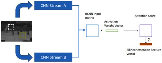
Figure 2. Bilinear attention flow diagram.

Table 2. Multistage network parameter information.

Input Image	3 × 299 × 299 (Channels × Width × Height)
Layer Name	Filter Size	Output Channels	Layer Name	Neurons
Conv1	9 × 9	16	Fusion	(40 × 1 × 1)
Mp1	2 × 2		FC1	1024
Conv2	7 × 7	32	FC	512
Mp2	2 × 2
Conv3	7 × 7	16
Conv4	7 × 7	8

Table 3. Multicolumn network parameter information.

Input Image	3 × 299 × 299 (Channels × Width × Height)
Layer Name	Branch 2			Branch 3					Layer Name	Neurons
Layer Name	Filter Size	Output Channels	Layer Name	Filter Size	Output Channels	Layer Name	Filter Size	Output Channels	Fusion	(30 × 1 × 1)
Conv1	9 × 9	16	Conv1	7 × 7	20	Conv1	5 × 5	24	FC1	1024
Mp1	2 × 2		Mp1	2 × 2		Mp1	2 × 2		FC	512
Conv2	7 × 7	32	Conv2	5 × 5	40	Conv2	3 × 3	48
Mp2	2 × 2		Mp2	2 × 2		Mp2	2 × 2
Conv3	7 × 7	16	Conv3	5 × 5	20	Conv3	3 × 3	24
Conv4	7 × 7	8	Conv4	5 × 5	10	Conv4	3 × 3	12

The MCNN architecture extracted different kernel features from the same image and fed pooled features to fully connected layers to reduce dimensionality. The details of the modified MCNN network architecture is described in Table 1. The resultant feature vector size was limited to 512 before the fusion with the BCNN attention feature vector.

In the MSCNN model architecture, the same input image was simultaneously fed to the feed-forward CNN network with multistage CNN feature aggregation. The proposed model improved MSCNN for efficient feature extraction. The modified multistage network architecture is explained in Figure 3. The MSCNN process’s first-stage convolution consisted of the first and second convolution operations. Then, the resultant output was concatenated with the second-stage convolution outputs (Conv3, Conv4). The MSCNN model improved feature information and reduced vanishing gradient issues in the network.

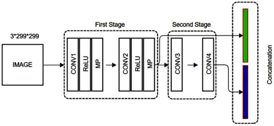
Figure 3. Modified MSCNN architecture.

3.3. Proposed Model Architecture

Both MCNN and MSCNN parallel streams’ feature vectors were concatenated with the BCNN attention vector before reaching the fully connected network. The process of bilinear model feature extraction and the operations of the bilinear attention feature vector generation are explained in Equations (1)–(7). The multicolumn (MC) and multistage (MS) feature vectors were concatenated with the bilinear attention feature vectors as:

$$C_{MC}=[f_{MCNN},f_{BCNN-att}]$$

(8)

$$C_{MS}=[f_{MS},f_{BCNN-att}]$$

(9)

where C and f represent concatenation and generated feature vectors, respectively. Both concatenated feature vectors have the same dimensions, as shown in Figure 1.

3.4. Fully Connected Network (FCN)

The primary feature extraction models were based on the pretrained densenet121/ EfficientNetV2 architectures with the bilinear CNN model (frozen model). Thus, the multistage and multicolumn models were trained with separate optimization functions, and we calculated the loss separately. For the training level, we used the Adam optimization [31] algorithm with a learning rate of 0.001 and a batch size of 40 for both models.

$$L_{Total}=L_{MC}+L_{MS}$$

(10)

(where L denotes the loss of the network). The feature concatenation and optimization loss calculation are shown in Equations (8)–(10).

4. Experiment Results and Discussion

The proposed model was based on the PyTorch [32] deep learning library and implemented with an Nvidia Geforce GTX 1660 GPU (6 GB dedicated memory) and AMD Ryzen 5 series processor with 16 GB of RAM. The publicly available UCSD [33], PETS2009 [34] and UMN [35] datasets were tested with our proposed model and results were compared with several other methods, such as CLBP [36] and MSCNN [28].

4.1. Dataset Preparation

The proposed models were tested with the publicly available crowd datasets UMN, PETS2009 and UCSD. The UMN dataset consists of two indoor crowd-monitoring video images Plaza1 and Plaza2. The PETS2009 provides different anomaly events and crowd density estimation videos with several viewpoints. In this experiment, we used data from one viewpoint with the different difficulty levels explained in the dataset. Finally, the UCSD ped1 and ped2 datasets were tested with the proposed model. The UCSD consist of several anomaly activities with different congestion levels. All frame-level annotation work was manually done and the segmentation of the congestion levels (VL—very Low, L—low, M—medium, H—high, VH—very high) was inspired from the TIS-MCMS work in [37]. The density levels for UCSD Ped1, UCSD Ped2 and PETS2009 and UMN Plaza1 and UMN Plaza2 are represented as $(VL<9,8<L<17,16<M<25,24<H<33,VH>32)$ and $(VL=0,0<L<4,$$4<M<7,6<H<11,VH>10)$, respectively.

The final training and the testing split were kept as a sixty-to-forty ratio for this work. The difficult level summarization and training and testing splits are mentioned in Table 4.

Table 4. Details of datasets’ splits for training and testing.

Dataset	Training Samples						Testing Samples
	VL	L	M	H	VH	Total	VL	L	M	H	VH	Total
UCSD-Ped1	2093	4171	1043	614	119	8040	1394	2715	690	480	82	5360
UCSD-Ped2	2113	4137	1016	785	107	8158	1374	2749	717	502	98	5440
PETS2009	49	128	156	114	290	737	46	86	111	70	179	492
UMN-Plaza1	113	503	123	93	190	1022	79	335	76	66	126	682
UMN-Plaza2	197	570	100	189	143	1199	125	371	75	142	87	800

4.1.1. UCSD Dataset

The UCSD benchmark dataset [33] consists of two different videos streams namely ped1 and ped2 with different viewpoints. The whole dataset consists of 16,000 and 4800 frames with a TIFF image format, respectively, and all images were converted to the JPEG image format. The UCSD dataset comprises sparse, occluded and low-resolution image data.

4.1.2. Pets2009 Dataset

The PETS2009 dataset [34] contains three different levels of complexity, namely L1, L2 and L3. Each difficulty level has four different viewpoints with two time segments. In this proposed experiment, we selected the time step data of each level for testing. Several samples of the complexity levels of each data set are shown in Figure 4.

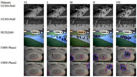
Figure 4. Examples of crowd scene of different density levels.

4.1.3. Umn Dataset

The UMN dataset [35] has a low complexity compared to the PETS2009 and UCSD datasets due to the stable indoor background scenario. The video recordings from UMN Plaza1 and Plaza2 surveillance cameras were prepared to monitor crowd density.

4.2. Model Training and Initialization of Parameters

The proposed model was fine-tuned on five crowd density levels by setting the parameters and hyperparameters. The training and validation batch sizes were set at 40 samples, the learning rate was kept at 0.001 and we used the Adam optimizer. In this approach, the model training performance was kept at its highest while avoiding overfitting when stopping the model training by adopting early stopping. The model training accuracy/loss and validation accuracy/loss performance are as shown in Figure 5, Figure 6, Figure 7 and Figure 8, respectively. The model with densenet121/EfficientNetV2 converged quickly with a high accuracy rate, as shown in Figure 5, Figure 6, Figure 7 and Figure 8.

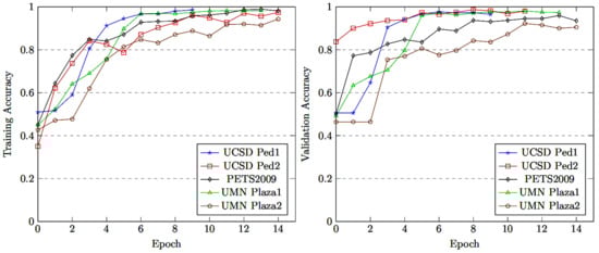
Figure 5. Training and validation accuracy of MCMS-BCNN-Attention + densenet121.

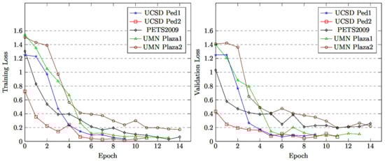
Figure 6. Training and validation loss of MCMS-BCNN-Attention + densenet121.

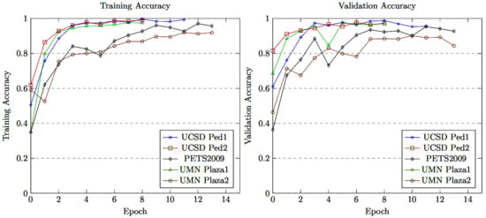
Figure 7. Training and validation accuracy of MCMS-BCNN-Attention + Efficientnetv2.

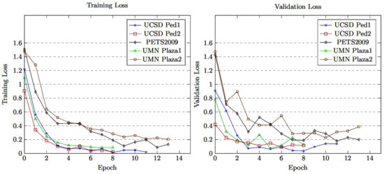
Figure 8. Training and validation loss of MCMS-BCNN-Attention + Efficientnetv2.

4.3. Evaluation Metrics

The performance of the model was evaluated as a multiclass classification scenario. Consequently, there were four different prediction states described as true positive (TP), true negative (TN), false positive (FP) and false negative (FN). All of the classes were successfully predicted with positive values, which meant that the true value of the class was positive, and the predicted value of the class was also positive. For example, if the density level for the real value of the class was medium density (M), while the predicted class was the same, this was identified as a true positive (TP). Moreover, a true negative (TN) was defined similarly as all the successfully predicted samples with negative values for which the true value of the class was negative and the predicted value of the class was also negative. For example, if the density level for the real value of the class was not medium density (M), and the predicted class was the same, then a false positive (FP) occurred when the actual class differed from the expected class, or when the expected class was positive and the actual class was negative. When the actual class was positive while the projected class was negatively defined, this was considered a false negative (FN).

4.4. Confusion Matrix

A confusion matrix was used to generalize the results of the classification method. For an unqualified number of observations in each class and more than two classes in the data sets, the correctness of the classification can be deceptive. Calculating the confusion matrix gives a clearer idea of what the classification model is doing right and where it is wrong. The two-class classification confusion matrix is shown in Table 5.

Table 5. Confusion Matrix explanation for binary classification.

	Predicted Class
Actual Class	Positive	Negative
Positive	True positive (TP)	False negative (FN)
Negative	false positive (FP)	True negative (TN)

To measure the performance of the model, we need to define a few measuring parameters, based on the multiclass classification confusion matrix. The performance evaluation was measured with the accuracy, precision, recall, $F_1$ score and kappa statistical measures explained in Equations (11)–(15).

$$Accuracy=\frac{TP+TN}{TP+TN+FP+FN}$$

(11)

$$Precision=\frac{TP}{TP+FP}$$

(12)

$$Recall=\frac{TP}{TP+FN}$$

(13)

$$F_{1}Score=2\times \frac{Precision\times Recall}{Precision+Recall}$$

(14)

Cohen’s kappa coefficient (k) is [38]:

$$k=\frac{P_o-P_e}{1-P_e}$$

(15)

where $P_o$ and $P_e$ represent observed agreement and expected agreement, respectively. This measurement shows how much better the classifier’s performance is compared to a balanced or unbalanced dataset.

5. Results Analysis

5.1. Benchmark Datasets Analysis

The performance comparison with existing approaches (Table 6) showed our model performance and that of other recent state-of-the-art approaches. Our proposed model achieved the best accuracy of 98.62 and 98.95 among the UCSD ped1 and UCSD ped2 datasets, respectively, compared with the existing CLBP, MSCNN, densenet121 and Efficientnetv2 methods. The total number of training frames was 8040 and the total number of testing frames was 5360; among those testing frames, there were 66 and 73 misclassified samples, respectively. The resultant confusion matrix is shown in Figure 9 and Figure 10. The proposed model achieved a good precision and recall rate compared with the other approaches. The proposed model trained with PETS2009 (737 training samples and 492 testing samples) achieved an accuracy of 96.97 with a total of 24 misclassified samples. The confusion matrix of the PETS2009 dataset with the proposed model is shown in Figure 11. The model achieved a better recall and precision than the other methods. This dataset had fewer samples compared with the other tested datasets with a high occlusion rate. Finally, the proposed model was tested on the UMN dataset and achieved an accuracy of 99.10 and 98.38 with a total of 17 and 17 incorrectly classified samples for UMN-Plaza1 and UMN-Plaza2, respectively. The relevant confusion matrix tables are shown in Figure 12 and Figure 13.

Table 6. Performance comparison with existing approaches.

Dataset	Approach	Performance (%)
		Accuracy	Precision	Recall	F1 Score	Kappa
UCSD Ped1	CLBP [39]	60.76	70.35	37.20	48.67	0.2238
	MSCNN [28]	97.48	98.70	96.22	97.45	0.9341
	densenet121 [1]	94.32	97.20	91.27	94.15	0.8673
	Efficientnetv2 [2]	97.03	98.55	95.46	96.98	0.9195
	Our (MCMS-BCNN-Attention+densenet121)	98.28	99.31	97.24	98.26	0.9646
	Our (MCMS-BCNN-Attention+Efficientnetv2)	98.62	99.51	97.21	98.61	0.9576
UCSD Ped2	CLBP [39]	62.19	73.80	37.78	49.98	0.2819
	MSCNN [28]	98.39	99.67	97.10	98.37	0.9834
	densenet121 [1]	92.88	96.96	88.55	92.56	0.8656
	Efficientnetv2 [2]	96.37	98.34	94.33	96.30	0.9231
	Our (MCMS-BCNN-Attention+densenet121)	98.95	99.54	98.36	98.95	0.9794
	Our (MCMS-BCNN-Attention+Efficientnetv2)	98.08	99.23	96.91	98.05	0.9629
PETS2009	CLBP [39]	86.80	95.37	77.33	85.42	0.8091
	MSCNN [28]	95.43	98.47	92.29	95.28	0.9222
	densenet121 [1]	93.17	97.02	89.09	92.88	0.8581
	Efficientnetv2 [2]	96.55	98.71	94.32	96.47	0.9327
	Our (MCMS-BCNN-Attention+densenet121)	96.38	98.64	94.06	96.30	0.9273
	Our (MCMS-BCNN-Attention+Efficientnetv2)	96.97	98.81	95.08	96.91	0.9353
UMN Plaza1	CLBP [39]	81.86	92.18	69.62	79.33	0.6857
	MSCNN [28]	97.79	99.24	96.31	97.76	0.9563
	densenet121 [1]	96.85	98.78	94.86	96.78	0.9404
	Efficientnetv2 [2]	98.50	99.41	97.57	98.48	0.9723
	Our (MCMS-BCNN-Attention + densenet121)	98.50	99.33	97.67	98.49	0.9640
	Our (MCMS-BCNN-Attention+Efficientnetv2)	99.10	99.41	98.78	99.09	0.9642
UMN Plaza2	CLBP [39]	60.36	70.18	36.01	47.60	0.2681
	MSCNN [28]	88.11	94.44	80.98	87.19	0.7841
	densenet121 [1]	94.11	97.34	90.70	93.90	0.8843
	Efficientnetv2 [2]	97.33	98.82	95.79	97.28	0.9402
	Our (MCMS-BCNN-Attention + densenet121)	98.38	99.12	97.63	98.37	0.9560
	Our (MCMS-BCNN-Attention+Efficientnetv2)	91.36	96.20	86.13	90.89	0.8525

Bold colour indicates the highest values.

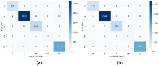
Figure 9. Confusion matrix heat map of UCSD Ped1 for (a) MCMS-BCNN-Attention+densenet121 and (b) MCMS-BCNN-Attention+Efficientnetv2.

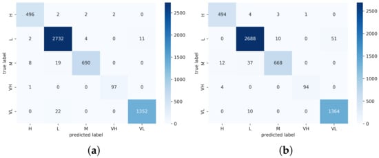
Figure 10. Confusion matrix heat map of UCSD Ped2 for (a) MCMS-BCNN-Attention+densenet121 and (b) MCMS-BCNN-Attention+Efficientnetv2.

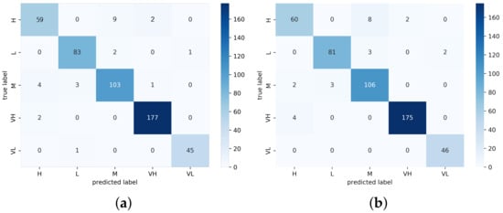
Figure 11. Confusion matrix heat map of PETS2009 for (a) MCMS-BCNN-Attention+densenet121 and (b) MCMS-BCNN-Attention+Efficientnetv2.

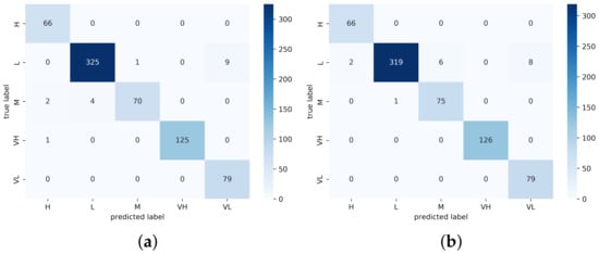
Figure 12. Confusion Matrix Heatmap of UMN Plaza 1 for (a) MCMS-BCNN-Attention+densenet121 and (b) MCMS-BCNN-Attention+Efficientnetv2.

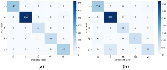
Figure 13. Confusion matrix heat map of UMN Plaza 2 for (a) MCMS-BCNN-Attention+densenet121 and (b) MCMS-BCNN-Attention+Efficientnetv2.

The comparison of the performance of the models in Table 6 clearly shows that the proposed method provided better results compared to the available models from the literature. In this approach, we selected different state-of-art models along with our multicolumn multistage approach. The comparison results clearly show that our work achieved the best performance either with densenet121 or Efficientnetv2 compared to existing methods. The proposed model achieved the best average kappa performance value over the five datasets with 0.9583.

5.2. Abnormal Event Detection and Classification

As mentioned earlier, crowd density level variation is also considered a crowd anomaly in a sequence. In this second approach, the network was transformed into a normal/abnormal classification problem. The same model was tested with the same parameters except for the final FCN layer, which was modified as a two-way classification. The results of testing both proposed feature extraction techniques (densenet121 and Efficientnetv2) are described in the sections below. In this approach, the abnormal activities were measured based on the UMN and PETS2009 dataset for detecting panic moments. The UMN dataset has three anomaly events (lawn, mall and plaza) with 7738 video frames with a 320 × 240 resolution. In this approach, the training and testing ratio was kept as sixty to forty as in previous work. However, final classification network was changed to a binary classification (normal/abnormal).

Experiments were also conducted on samples from the PETS2009 S3 motion flow walking and running video segments shown in Figure 14. The model performance was tested with video sequences 14–16 (walk and run) and 14–33 (gather and evacuate), respectively. The performance was measured by calculating the AUC (area under the curve) [40] using the ROC (receiver operating characteristic) [40] curve. The AUC measures the area under the ROC curve. The TPR (true positive rate) and FPR (false positive rate) calculations are explained in Equations (16) and (17). The ROC curve was plotted by using TPR against FPR values.

$$TPR=\frac{TP}{TP+FN}$$

(16)

$$FPR=\frac{FP}{FP+TN}$$

(17)

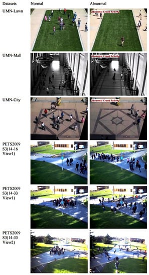
Figure 14. Sample frames for UMN and PETS2009 datasets abnormal activity.

We evaluated UMN’s activities in the lawn, shopping mall and city urban event (indoor/outdoor) segments with existing approaches. The performance results were compared with our model (MCMS-BCNN-Attention), as shown in Table 7, which achieved the best AUC of 1.0. In this approach, the separation of actions is an extremely difficult task when people walk normally and suddenly start running to evacuate. However, our proposed model architecture with Efficientnetv2-based feature extraction achieved perfect results among all the other works. In the PETS2009 dataset, we monitored two activities such as walking/running and gathering/disappearing. We maintained the same sixty-to-forty ratio as when splitting training and testing into all original datasets’ segments for the experiment. The effectiveness of our approach compared to existing recent works is shown in Table 7, and the MCMS-BCNN-Attention model reached an AUC of 1.0, yielding the best performance.

Table 7. Performance comparison of the proposed approach with existing techniques on UMN and PETS2009 datasets.

Dataset	Method	AUC ( Lawn/Mall/City)	AUC Total
UMN	Wang et al. [41]	0.9981/0.9724/0.9888	0.9864
	Cong et al. [42]	0.995/0.975/0.964	0.979
	Wang et al. [43]	0.9779/0.9223/0.9849	0.9617
	Susan et al. [44]	0.997/0.89/0.962	0.945
	Zhang et al. [45]	0.992/0.986/0.979	0.985
	Kaltsa et al. [46]	0.9959/0.9338/0.9808	0.9702
	Xu et al. [47]	0.9861/0.9864/0.975	0.9825
	Mu et al. [48]	0.996/98.3/99.1	0.99
	Ilyas et al. [49]	0.9808/0.9955/0.9935	0.990
	Du Y [50]	0.998/0.992/0.995	0.9950
	Sing et al. [51]	0.9928/0.9885/0.9995	0.9936
	Our (MCMS-BCNN-Attention + densenet121)	0.9615/0.9981/0.9056	0.9505
	Our (MCMS-BCNN-Attention+Efficientnetv2)	1.00/99.25/99.33	0.9953
PETS2009	Method	AUC (14-16 View_1)	AUC (14-33 View_1,
			View_2,View_3)
	Xu et al. [52]		0.94
	Zhu et al. (Optical flow) [53]		0.81
	Zhu et al. (SFM) [53]		0.94
	Ilyas et al. [49]	-	0.94
	Sing et al. [51]	0.9788	-
	Du Y [50]	0.9780	-
	Our (MCMS-BCNN-Attention + densenet121)	0.9895	0.9666
	Our (MCMS-BCNN-Attention+Efficientnetv2)	1.0	1.0

Bold colour indicates the highest values.

6. Conclusions

In this study, we introduced a novel BCNN attention network with a densenet121/ Efficientnetv2 architecture as a transfer learning model to extract feature vectors and achieve the best accuracy rate. Both the modified multistage and multicolumn models were trained to optimize the classification network. The experiments compared our method with recent state-of-art methods and evaluated performance with metrics such as accuracy, precision, recall, F1 score and Cohen’s kappa values. The proposed feature extraction method significantly improved the anomaly congestion detection as shown in the comparison of Table 6. The evaluated datasets contained diverse video quality levels and different viewpoints, and the proposed model achieved a good performance consistency in all scenarios. Moreover, the detection of the abnormal activity (panic moments) also achieved good results. Future dense activity detection models need to be enhanced with an autoencoder-based approach to achieve better video activity detection. The performance measures are shown in Table 7. The clarity of the surveillance video and the distance to the viewpoint with multiview aspects need to be considered for future improvements and better detection results.

References

- Huang, G.; Liu, Z.; Van Der Maaten, L.; Weinberger, K.Q. Densely connected convolutional networks. In Proceedings of the IEEE Conference on Computer Vision and Pattern Recognition 2017, Honolulu, HI, USA, 21–26 July 2017; pp. 4700–4708. [Google Scholar]
- Tan, M.; Le, Q. Efficientnetv2: Smaller models and ster training. In Proceedings of the International Conference on Machine Learning, PMLR, Virtual Event, 18–24 July 2021; pp. 10096–10106. [Google Scholar]
- Zhang, Y.; Zhou, D.; Chen, S.; Gao, S.; Ma, Y. Single-image crowd counting via multi-column convolutional neural network. In Proceedings of the IEEE Conference on Computer Vision and Pattern Recognition, Las Vegas, NV, USA, 27–30 June 2016; pp. 589–597. [Google Scholar]
- Aldayri, A.; Albattah, W. Taxonomy of Anomaly Detection Techniques in Crowd Scenes. Sensors 2022, 22, 6080. [Google Scholar] [CrossRef] [PubMed]
- Wang, T.; Miao, Z.; Chen, Y.; Zhou, Y.; Shan, G.; Snoussi, H. Aed-net: An abnormal event detection network. Engineering 2019, 5, 930–939. [Google Scholar] [CrossRef]
- Biswas, S.; Babu, R.V. Anomaly detection via short local trajectories. Neurocomputing 2017, 242, 63–72. [Google Scholar] [CrossRef]
- Bera, A.; Kim, S.; Manocha, D. Realtime anomaly detection using trajectory-level crowd behavior learning. In Proceedings of the IEEE Conference on Computer Vision and Pattern Recognition Workshops, Las Vegas, NV, USA, 27–30 June 2016; pp. 50–57. [Google Scholar]
- Maiorano, F.; Petrosino, A. Granular trajectory based anomaly detection for surveillance. In Proceedings of the 2016 23rd International Conference on Pattern Recognition (ICPR), Cancun, Mexico, 4–8 December 2016; pp. 2066–2072. [Google Scholar]
- Biswas, S.; Babu, R.V. Short local trajectory based moving anomaly detection. In Proceedings of the 2014 Indian Conference on Computer Vision Graphics and Image Processing, Bangalore, India, 14–18 December 2014; pp. 1–8. [Google Scholar]
- Zhao, K.; Liu, B.; Li, W.; Yu, N.; Liu, Z. Anomaly detection and localization: A novel two-phase framework based on trajectory-level characteristics. In Proceedings of the 2018 IEEE International Conference on Multimedia & Expo Workshops (ICMEW), San Diego, CA, USA, 23–27 July 2018; pp. 1–6. [Google Scholar]
- Zhang, X.; Ma, D.; Yu, H.; Huang, Y.; Howell, P.; Stevens, B. Scene perception guided crowd anomaly detection. Neurocomputing 2020, 414, 291–302. [Google Scholar] [CrossRef]
- Hao, Y.; Xu, Z.J.; Liu, Y.; Wang, J.; Fan, J.L. Effective crowd anomaly detection through spatio-temporal texture analysis. Int. J. Autom. Comput. 2019, 16, 27–39. [Google Scholar] [CrossRef]
- Li, N.; Chang, F. Video anomaly detection and localization via multivariate Gaussian fully convolution adversarial autoencoder. Neurocomputing 2019, 369, 92–105. [Google Scholar] [CrossRef]
- Li, X.; Li, W.; Liu, B.; Liu, Q.; Yu, N. Object-oriented anomaly detection in surveillance videos. In Proceedings of the 2018 IEEE International Conference on Acoustics, Speech and Signal Processing (ICASSP), Calgary, AB, Canada, 15–20 April 2018; pp. 1907–1911. [Google Scholar]
- Si, C.; Chen, W.; Wang, W.; Wang, L.; Tan, T. An attention enhanced graph convolutional lstm network for skeleton-based action recognition. In Proceedings of the IEEE/CVF Conference on Computer Vision and Pattern Recognition 2019, Long Beach, CA, USA, 15–20 June 2019; pp. 1227–1236. [Google Scholar]
- Lloyd, K.; Rosin, P.L.; Marshall, D.; Moore, S.C. Detecting violent and abnormal crowd activity using temporal analysis of grey level co-occurrence matrix (GLCM) -based texture measures. Mach. Vis. Appl. 2017, 28, 361–371. [Google Scholar] [CrossRef]
- Hasan, M.; Choi, J.; Neumann, J.; Roy-Chowdhury, A.K.; Davis, L.S. Learning temporal regularity in video sequences. In Proceedings of the IEEE Conference on Computer Vision and Pattern Recognition 2016, Las Vegas, NV, USA, 27–30 June 2016; pp. 733–742. [Google Scholar]
- Luo, W.; Liu, W.; Gao, S. Remembering history with convolutional lstm for anomaly detection. In Proceedings of the 2017 IEEE International Conference on Multimedia and Expo (ICME) 2017, Hong Kong, China, 10–14 July 2017; pp. 439–444. [Google Scholar]
- Gong, D.; Liu, L.; Le, V.; Saha, B.; Mansour, M.R.; Venkatesh, S.; Hengel, A.V. Memorizing normality to detect anomaly: Memory-augmented deep autoencoder for unsupervised anomaly detection. In Proceedings of the IEEE/CVF International Conference on Computer Vision 2019, Seoul, Republic of Korea, 27 October–2 November 2019; pp. 1705–1714. [Google Scholar]
- Wu, C.; Shao, S.; Tunc, C.; Hariri, S. Video anomaly detection using pre-trained deep convolutional neural nets and context mining. In Proceedings of the 2020 IEEE/ACS 17th International Conference on Computer Systems and Applications (AICCSA), Antalya, Turkey, 2–5 November 2020; pp. 1–8. [Google Scholar]
- Huang, S.; Huang, D.; Zhou, X. Learning multimodal deep representations for crowd anomaly event detection. Math. Probl. Eng. 2018, 2018, 6323942. [Google Scholar] [CrossRef]
- Wang, T.; Qiao, M.; Zhu, A.; Shan, G.; Snoussi, H. Abnormal event detection via the analysis of multi-frame optical flow information. Front. Comput. Sci. 2020, 14, 304–313. [Google Scholar] [CrossRef]
- Singh, K.; Rajora, S.; Vishwakarma, D.K.; Tripathi, G.; Kumar, S.; Walia, G.S. Crowd anomaly detection using aggregation of ensembles of fine-tuned convnets. Neurocomputing 2020, 371, 188–198. [Google Scholar] [CrossRef]
- Sultani, W.; Chen, C.; Shah, M. Real-world anomaly detection in surveillance videos. In Proceedings of the IEEE Conference on Computer Vision and Pattern Recognition 2018, Salt Lake City, UT, USA, 18–22 June 2018; pp. 6479–6488. [Google Scholar]
- Marsden, M.; McGuinness, K.; Little, S.; O’Connor, N.E. Resnetcrowd: A residual deep learning architecture for crowd counting, violent behaviour detection and crowd density level classification. In Proceedings of the 2017 14th IEEE international conference on advanced video and signal based surveillance (AVSS), Lecce, Italy, 29 August 2017–1 September 2017; pp. 1–7. [Google Scholar]
- Ratre, A. Taylor series based compressive approach and Firefly support vector neural network for tracking and anomaly detection in crowded videos. J. Eng. Res. 2019, 7, 115–137. [Google Scholar]
- Feng, Y.; Yuan, Y.; Lu, X. Learning deep event models for crowd anomaly detection. Neurocomputing 2017, 219, 548–556. [Google Scholar] [CrossRef]
- Fu, M.; Xu, P.; Li, X.; Liu, Q.; Ye, M.; Zhu, C. Fast crowd density estimation with convolutional neural networks. Eng. Appl. Artif. Intell. 2015, 43, 81–88. [Google Scholar] [CrossRef]
- A Comprehensive Hands-on Guide to Transfer Learning with Real-World Applications in Deep Learning. Available online: https://towardsdatascience.com/a-comprehensive-hands-on-guide-to-transfer-learning-with-real-world-applications-in-deep-learning-212bf3b2f27a (accessed on 1 November 2022).
- Lin, T.Y.; Roy Chowdhury, A.; Maji, S. Bilinear cnn models for fine-grained visual recognition. In Proceedings of the IEEE International Conference on Computer Vision 2015, Santiago, Chile, 7–13 December 2015; pp. 1449–1457. [Google Scholar]
- Kingma, D.P.; Ba, J. Adam: A method for stochastic optimization. arXiv 2014, arXiv:1412.6980. [Google Scholar]
- Paszke, A.; Gross, S.; Massa, F.; Lerer, A.; Bradbury, J.; Chanan, G.; Killeen, T.; Lin, Z.; Gimelshein, N.; Antiga, L.; et al. Pytorch: An imperative style, high-performance deep learning library. In Proceedings of the Advances in Neural Information Processing Systems 32 (NeurIPS 2019), Vancouver, BC, Canada, 8–14 December 2019; Neural Information Processing Systems Foundation, Inc. (NeurIPS): San Diego, CA, USA, 2019. Available online: https://proceedings.neurips.cc/paper/2019/file/bdbca288fee7f92f2bfa9 f7012727740-Paper.pdf (accessed on 2 December 2022).
- UCSD Anomaly Detection Dataset. Available online: http://www.svcl.ucsd.edu/projects/anomaly/dataset.html (accessed on 7 November 2022).
- PETS 2009 Benchmark Data. Available online: http://cs.binghamton.edu/mrldata/pets2009 (accessed on 7 November 2022).
- Monitoring Human Activity-Action Recognition. Available online: http://mha.cs.umn.edu/projrecognition.shtml (accessed on 7 November 2022).
- Alanazi, A.A.; Bilal, M. Crowd density estimation using novel feature descriptor. arXiv 2019, arXiv:1905.05891. [Google Scholar]
- Tripathy, S.K.; Srivastava, R. A real-time two-input stream multi-column multi-stage convolution neural network (TIS-MCMS-CNN) for efficient crowd congestion-level analysis. Multimed. Syst. 2020, 26, 585–605. [Google Scholar] [CrossRef]
- Shmueli, B.; Multi-Class Metrics Made Simple, Part III: The Kappa Score (Aka Cohen’s Kappa Coefficient). Medium. Towards Data Science. 2020. Available online: https://towardsdatascience.com/multi-class-metrics-made-simple-the-kappa-score-aka-cohens-kappa-coefficient-bdea137af09c (accessed on 2 December 2022).
- Chen, C.; Zhang, B.; Su, H.; Li, W.; Wang, L. Land-use scene classification using multi-scale completed local binary patterns. Signal Image Video Process. 2016, 10, 745–752. [Google Scholar] [CrossRef]
- Bradley, A.P. The use of the area under the ROC curve in the evaluation of machine learning algorithms. Pattern Recognit. 1997, 30, 1145–1159. [Google Scholar] [CrossRef]
- Wang, T.; Qiao, M.; Chen, Y.; Chen, J.; Zhu, A.; Snoussi, H. Video feature descriptor combining motion and appearance cues with length-invariant characteristics. Optik 2018, 157, 1143–1154. [Google Scholar] [CrossRef]
- Cong, Y.; Yuan, J.; Liu, J. Sparse reconstruction cost for abnormal event detection. In Proceedings of the Computer Vision and Pattern Recognition 2011, Colorado Springs, CO, USA, 20–25 June 2011; pp. 3449–3456. [Google Scholar]
- Wang, T.; Qiao, M.; Deng, A.; Zhou, Y.; Wang, H.; Lyu, Q.; Snoussi, H. Abnormal event detection based on analysis of movement information of video sequence. Optik 2018, 152, 50–60. [Google Scholar] [CrossRef]
- Susan, S.; Hanmandlu, M. Unsupervised detection of nonlinearity in motion using weighted average of non-extensive entropies. Signal Image Video Process. 2015, 9, 511–525. [Google Scholar] [CrossRef]
- Zhang, X.; Yang, S.; Tang, Y.Y.; Zhang, W. A thermodynamics-inspired feature for anomaly detection on crowd motions in surveillance videos Multimed. Tools Appl. 2020, 75, 8799–8826. [Google Scholar] [CrossRef]
- Kaltsa, V.; Briassouli, A.; Kompatsiaris, I.; Hadjileontiadis, L.J.; Strintzis, M.G. Swarm intelligence for detecting interesting events in crowded environments. IEEE Trans. Image Process. 2015, 24, 2153–2166. [Google Scholar] [CrossRef] [PubMed]
- Xu, Y.; Lu, L.; Xu, Z.; He, J.; Zhou, J.; Zhang, C. Dual-channel CNN for efficient abnormal behavior identification through crowd feature engineering. Mach. Vis. Appl. 2019, 30, 945–958. [Google Scholar] [CrossRef]
- Mu, H.; Sun, R.; Yuan, G.; Li, J.; Wang, M. Crowd behavior detection in videos using statistical physics. In Proceedings of the 2021 International Conference on Data Mining Workshops (ICDMW), Auckland, New Zealand, 7–10 December 2021; pp. 389–397. [Google Scholar]
- Ilyas, Z.; Aziz, Z.; Qasim, T.; Bhatti, N.; Hayat, M.F. A hybrid deep network based approach for crowd anomaly detection. Multimed. Tools Appl. 2021, 80, 24053–24067. [Google Scholar] [CrossRef]
- Du, Y. An anomaly detection method using deep convolution neural network for vision image of robot. Multimed. Tools Appl. 2020, 79, 9629–9642. [Google Scholar] [CrossRef]
- Singh, G.; Kapoor, R.; Khosla, A. Optical flow-based weighted magnitude and direction histograms for the detection of abnormal visual events using combined classifier. Int. J. Cogn. Inform. Nat. Intell. (IJCINI) 2021, 15, 12–30. [Google Scholar] [CrossRef]
- Xu, J.; Denman, S.; Fookes, C.; Sridharan, S. Unusual scene detection using distributed behaviour model and sparse representation. In Proceedings of the 2012 IEEE Ninth International Conference on Advanced Video and Signal-Based Surveillance, Beijing, China, 18–21 September 2012; pp. 48–53. [Google Scholar]
- Zhu, X.; Liu, J.; Wang, J.; Fu, W.; Lu, H. Weighted interaction force estimation for abnormality detection in crowd scenes. In Asian Conference on Computer Vision; Springer: Berlin/Heidelberg, Germany, 2012; pp. 507–518. [Google Scholar]
Disclaimer/Publisher’s Note: The statements, opinions and data contained in all publications are solely those of the individual author(s) and contributor(s) and not of MDPI and/or the editor(s). MDPI and/or the editor(s) disclaim responsibility for any injury to people or property resulting from any ideas, methods, instructions or products referred to in the content. |
© 2022 by the authors. Licensee MDPI, Basel, Switzerland. This article is an open access article distributed under the terms and conditions of the Creative Commons Attribution (CC BY) license (https://creativecommons.org/licenses/by/4.0/).