Abstract
This paper proposes a structural damage detection method based on one-dimensional convolutional neural network (CNN). The method can automatically extract features from data to detect structural damage. First, a three-layer framework model was designed. Second, the displacement data of each node was collected under the environmental excitation. Then, the data was transformed into the interlayer displacement to form a damage dataset. Third, in order to verify the feasibility of the proposed method, the damage datasets were divided into three categories: single damage dataset, multiple damage dataset, and damage degree dataset. The three types of damage dataset can be classified by the convolutional neural network. The results showed that the recognition accuracy is above 0.9274. Thereafter, a visualization tool called “t-SNE” was employed to visualize the raw data and the output data of the convolutional neural network. The results showed that the feature extraction ability of CNN is excellent. However, there are many hidden layers in a CNN. The outputs of these hidden layers are invisible. In the last section, the outputs of hidden layers are visualized to understand how the convolutional neural networks work.
1. Introduction
Structural reliability is a comprehensive evaluation indicator of structural performance, including reliability, stability, and durability. A structure must be able to withstand natural disasters, such as earthquakes and typhoons. As a result of the material aging and environmental corrosion, the structure will inevitably face a variety of structural damage, such as cracking, spalling, and so on. These damages will affect the reliability of the building structure and even cause collapse. Therefore, health monitoring systems are widely used in various structures such as bridges [1,2], harbors [3], high-rise buildings [4,5,6], large space structures [7], and so on. A health monitoring system includes data acquisition system, transmission system, data processing system, and safety assessment system [8]. A data acquisition system contains many sensors such as accelerometers, displacement meters, inclinometers, strain gauges, and stress gauges. These sensors collect huge amounts of data for health monitoring systems. The transmission systems are mainly divided into wired transmission system and wireless transmission system. With the continuous development of transmission technology, it provides convenience for health monitoring systems. In addition, the data processing system is the core of the health monitoring system. It determines the effect of implementation of the health monitoring system and provides the basis for structural safety assessment.
The purpose of the data processing system is to identify the degree and location of structural damage. According to the theory of structural dynamics, structural damage can change the structural dynamic characteristics, such as the mode shape, frequency, and stiffness of the structure [9]. The degree and location of the damage can be detected by the change of these modal parameters. Therefore, some structural damage detection methods [10,11,12,13,14] based on modal identification have been studied. These methods focus on the changes of the structural modal parameters. They can analyze the signal in both time and frequency domains. However, the frequency domain analysis of these methods mainly relies on the Fourier transform. When the Fourier transform extracts the frequency spectrum from the signal, all the time domain information of the signal is used. It lacks the ability to analyze the local features of the signal [15]. Nevertheless, the wavelet analysis has solved this problem. It uses a variable window to process the signal in both time and frequency domains [16]. The effect of structural damage on the output signal is very weak. The ability of wavelet analysis to extract local features can be used to identify the effect. Therefore, wavelet analysis is also widely used in the field of damage identification, such as damage recognition based on the principle of wavelet singularity detection [17] and damage identification by wavelet packet energy method [18].
Another type of damage identification technology is based on statistical information. At present, the mainstream structure in the building structure is the frame structure. The two most important components in the frame structure are beam and column. Thus, the possible damage locations of structures are limited. Collecting a large amount of information for limited damage is the advantage of statistical learning theory. This type of method collects the output signal of the structure under different conditions. Different damages have different effects on the output signal. Therefore, the damage identification problem can be converted into a classification problem. For example, the support vector machine [19,20,21,22] takes the characteristic parameters of the signal as the input for the network and takes the degree and location of the structural damage as the outputs for the network. Then, the structural damage dataset is established. One part of the dataset is used as a training set and the other is used as a validation set. The training set is used to train the model, and the validation set is used to verify the detection performance of the training model. Then, the model is used to identify the structural damage. Furthermore, support vector machines are friendly to small datasets. However, the dataset needs to be processed by feature engineering [23,24]. The core of feature engineering is the method of feature extraction. It includes data preprocessing, feature selection, and dimensionality reduction. Different types of damage extract different features. So, feature engineering requires a lot of experimental experience. The feature selection of data directly determines the accuracy of this type of damage identification method. Therefore, a damage identification method without having to rely on feature engineering is required.
In recent years, convolutional neural networks have made remarkable achievements in the field of object detection. The convolutional neural network was first proposed in 1985 [25]. It was then applied to the multi-layer neural network, and the first convolutional neural network model was proposed [26]. However, the computational complexity of the model is too large. The development of convolutional neural networks has been stagnant. Until 2006, Hinton pointed out that multiple-hidden-layer neural networks have superior feature learning ability [27]. Since then, convolutional neural networks have developed continuously and have achieved amazing results in various fields [28]. The convolutional neural networks extract features by a series of layers such as convolutional layer and pooling layer. It can realize the end-to-end object detection, and the training model can be used to directly classify the input data. The method requires a large amount of data. The existing health monitoring system generates a large amount of monitoring data. How to use them effectively has become an important issue. The big data and convolutional neural networks can improve the accuracy of structural damage detection [29,30,31]. In 2017, Cha et al. [32] applied the convolutional neural network to crack detection. They can identify and locate cracks in the image. Then, deep learning is widely used in the field of damage detection [33]. Hurricanes as a natural disaster often cause severe damage to infrastructure [34]. Kakareko et al. [35] used CNN to identify trees and their types from satellite images. The tree damage assessment module was used to calculate the vulnerability function and thus estimate the likelihood of road closure. Amit et al. [36] proposed an automatic disaster detection system based on CNN and satellite images that can be used to identify landslides and floods. Experimental results showed that the system has an average identification accuracy of between 80% and 90% for disasters. Zhao et al. [37] proposed a method that combines Mask R-CNN and building boundary regularization to extract and localize building polygons from satellite images. Experimental results showed that the proposed method produces better regularized polygons. Cha et al. [38] proposed a Faster R-CNN and machine vision-based damage identification method for five different types of surface damage. The results showed that the proposed method has an average precision of 87.8% and the detection speed of 0.03 s per image. However, these methods belong to supervised learning, which requires data with labels. In contrast, unsupervised learning does not require data labeling, which greatly improves the engineering application scenario. In the unsupervised mode, structural damage detection is referred to as unsupervised novelty detection. Cha et al. [39] proposed a fast-clustering algorithm based on density peaks for structural damage detection and localization. A Gaussian kernel function with radius was introduced to calculate the local density of data points, and a new damage-sensitive feature was proposed. Wang et al. [40] proposed an unsupervised learning method based on deep auto-encoder with a one-class support vector machine. The experimental results showed that the proposed method could achieve high accuracy in structural damage detection and also complete minor damage identification with an accuracy of over 96.9%.
This paper proposes a frame structure damage detection method based on a one-dimensional convolutional neural network. First, a three-layer framework model was designed. Second, the displacement data of each node was collected under the environmental excitation. Additionally, the data was transformed into the interlayer displacement, which formed a damage dataset. Third, the damage datasets were classified by the convolutional neural network. This research’s content is described as follows: Section 2 introduces the overall framework of the method and the architecture of the proposed CNN; Section 3 implements the single damage location detection; Section 4 implements the multiple damage location detection; Section 5 implements damage degree detection; Section 6 visualizes the convolutional neural network; Section 7 concludes this article.
2. Formulation of Analytical Model
In this paper, a structure damage detection method based on one-dimensional convolutional neural network has been proposed. The overall framework of the method is shown in Figure 1. First, a three-layer framework model was built by ABAQUS. Damage was simulated by decreasing the stiffness of the column. Then, the displacement data of each node was collected under the environmental excitation. The data was transformed into the interlayer displacement, which formed a damage dataset. The dataset was entered into the proposed convolutional neural network to identify the location and degree of structural damage. In order to verify the identification effect of convolutional neural networks, three datasets (single damage dataset, multiple damage dataset, and damage degree dataset) were generated.
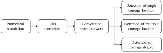
Figure 1.
The overall framework.
2.1. Numerical Simulation
A three-dimensional finite element model was established by ABAQUS. The seismic fortification intensity is 8 degrees, the layer height is 4500 mm, and the span is 7200 mm. The model and the number of beams, columns, and joints are shown in Figure 2. Both columns and beams are made of Q235 steel. Further details of the beams and columns are shown in Table 1.
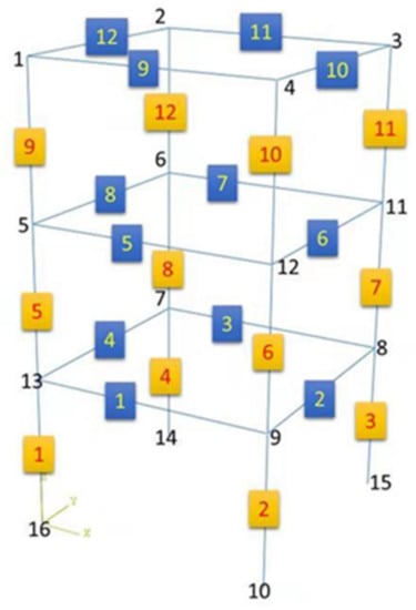
Figure 2.
The model and the number of beams, columns, and joints.

Table 1.
The parameters of beams and columns.
As a result of material aging and environmental corrosion, the structure will inevitably face a variety of structural damage such as cracking, spalling and so on. These damages can change the stiffness of the components and affect the safety of the building structure. In this paper, damage was simulated by decreasing the stiffness of the column. In the detection of damage location, the stiffness of column 1, column 6, and column 11 was reduced by 20%. In the detection of damage degree, the stiffness of column 1 was reduced by 10%, 20%, 30% and 40%, respectively.
2.2. Dataset Generation
The displacement data of each node was collected under environmental excitation. The number of displacement data that each node collects is 19,950, and the acquisition frequency is 100 Hz. The data were transformed into the interlayer displacement. The interlayer displacement data of 12 nodes (1, 2, 3, 4, 5, 6, 7, 8, 9, 11, 12 and 13) were selected as the dataset. The number of interlayer displacement data that each sample contains is 50. There is no overlap between each sample. Thus, the number of each type of sample is 399. The generation process of each type of sample is shown in Figure 3. In this paper, the displacement of each node was used as the input. Therefore, the detection of building displacements is a very important topic. For large infrastructures, it is not practicable to use ordinary laser displacement sensors to monitor the displacement. In order to improve the feasibility and convenience of detection, machine vision methods can be used to obtain the displacement data of each node. For instance, the displacement detection method based on optical flow and unscented Kalman filter can accomplish the displacement of large infrastructures with low noise levels [41].
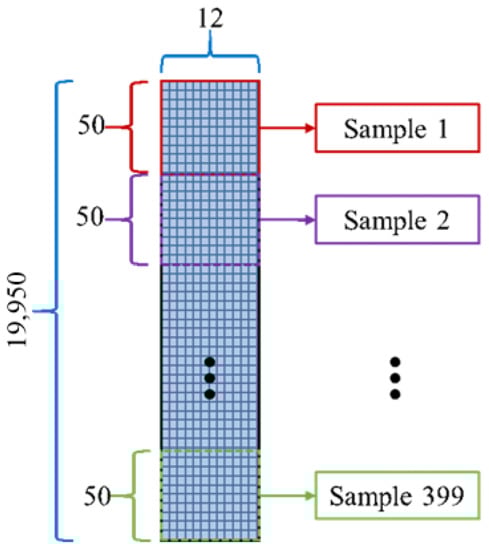
Figure 3.
Sample generation.
2.3. Convolutional Neural Networks
A typical convolutional neural network consists of a convolutional layer, a pooling layer, and a fully connected layer. These layers work together to extract features from the data. Then, the classification is completed by the fully connected layer. Through the series of operations, the convolutional neural network can reduce the dimensionality of data and make it easier to be trained. The details of the proposed convolutional neural network architecture are shown in Table 2.
Table 2.
The details of the proposed CNN architecture.
- (1)
- Convolutional layer
A traditional neural network consists of an input layer, a hidden layer, and an output layer. There are many neurons in each layer. Additionally, the neurons between two adjacent layers are fully connected. Therefore, it produces a large number of parameters. Excessive parameters will cause gradient dispersion. Convolution can reduce parameters in the neural network and improve learning efficiency. Therefore, the convolutional layer is the most important component of the convolutional neural network. Two-dimensional convolution is often used in image processing. However, the input data are interlayer displacement in this paper, and one-dimensional convolution is very suitable for this kind of damage detection. The data is inputted into the convolutional layer, and the convolutional kernel in the convolutional layer and the input data are convoluted. The input shape of the first convolutional layer is 50 × 12, the kernel size is 5 × 12, the kernel number is 32. Each convolution operation only processes a part of the input data. The convolutional kernel starts at the upper left corner of the input data, and the parameters of the convolutional kernel are multiplied by the parameters of the coverage area. Then, the multiplied values are summed. The convolutional kernel moves one element (stride = 1) down for the next convolution. The initial parameters within the convolutional kernel are randomly generated. In this convolutional neural network, each convolutional kernel can generate a 46 × 1 matrix with input data. Thus, the output shape of the first convolutional layer is 46 × 32. The convolution operation diagram is show in Figure 4.
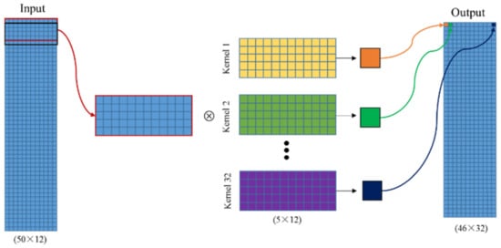
Figure 4.
Convolution operation diagram.
- (2)
- Activation function
In order to simulate the human nervous system, a neural network is proposed. The human nervous system responds only to some neurons. The activation function is also intended to activate some neurons. The activation of neurons is determined by the activation function. The activation function is divided into linear activation function and nonlinear activation function. Linear activation functions can only provide linear mapping capabilities and do not improve the expressive power of the network. Therefore, the nonlinear activation function has been widely used. Common nonlinear activation functions are sigmoid, tanh, and rectified linear unit (ReLU). These nonlinear activation functions are shown in Figure 5.
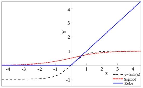
Figure 5.
Activation function.
As can be seen from Figure 5, the derivatives of sigmoid and tanh are zero when x approaches infinity. This situation easily causes the vanishing gradient problem, and the state of network cannot be updated. However, the ReLU activation function has a relatively broad excitatory boundary. It solves the vanishing gradient problem. Additionally, the ReLU activation function is the most used activation function in deep learning.
- (3)
- Pooling layer
The role of the pooling layer is to reduce the size of the feature map. The pooling layer is similar to the convolutional layer, it also has a kernel. However, the pooling kernel does not contain any parameters. The pooling layer is divided into maximum pooling layer and mean pooling layer. The pooling operation starts at the upper left corner of the input data. For the maximum pooling, the maximum value of all the parameters in the coverage area is outputted. For the mean pooling, the mean value of all the parameters in the coverage area is outputted. The movement of the pooling kernel is the same as the movement of the convolutional kernel. The pooling layer is also called the down sampling layer, which can reduce the parameters in the feature map and improve the training efficiency of the model.
- (4)
- Fully connected layer
The fully connected layer can be seen as a “classifier” in the convolutional neural network. The convolutional layer maps the raw data to feature space of the hidden layer, and the fully connected layer maps the learned distributed feature to the sample tag space. Each neuron in the fully connected layer is connected to all neurons in the anterior layer. The output signal of the fully connected layer is passed to the objective function (loss function) for classification. A dense layer is a classic fully connected neural network layer. The output shape of last fully connected layer is 4 in this CNN. This value is consistent with the number of categories.
- (5)
- Loss function
The inconsistency between the predicted value and the actual label of each sample is called loss. The smaller the loss, the better the detection performance of the training model. The function that is used to calculate the loss is called the loss function. The most used loss function in deep learning is softmax, which is used for multi-classification problems. It can map the outputs of multiple neurons into intervals of 0 to 1. These values can be understood as prediction probabilities. The label corresponding to the highest probability is outputted as our prediction result.
3. Single Damage Location Detection
3.1. Single Damage Dataset
In the single damage location detection, the stiffness of column 1, column 6, and column 11 was reduced by 20%. The displacement data of each node was collected and converted into interlayer displacement. The single damage dataset includes four categories: “c0”, “c1”, “c6”, and “c11”. The category “c0” means that there are no damaged columns; “c1” means that the damaged column is column 1; “c6” means that the damaged column is column 6; “c11” means that the damaged column is column 11. The data in the dataset were obtained from the finite element model. The specific parameters in the finite element model were set according to the damage types mentioned above. Displacement of each node in the finite element model under environmental excitation was collected. Meanwhile, the displacement of each node was converted into interlayer displacement, i.e., the interlayer displacement of 12 nodes was obtained. The acquisition frequency was set to 100 Hz. Each sample contains 50 data points, which is 0.5 s of acquisition time. Each sample in the dataset is a matrix of 12 × 50. Among them, 12 represents 12 nodes and 50 represents 50 data points. The number of samples is 399 in each category, and the dataset contains a total of 1596 samples. After these samples are randomly sorted, 1200 samples were used for training and verification, 396 samples were used as test set.
3.2. Detection Result
The training set and the valid set are inputted into the proposed convolutional neural network. The training accuracy and the valid accuracy increase with the increase of the number of iteration steps, and finally reach a stable state. Training accuracy and valid accuracy are shown in Figure 6. When the number of iteration epoch is 100, the training accuracy is 1.0 and the valid accuracy is 0.9953. The detection accuracy has met the requirements of engineering.
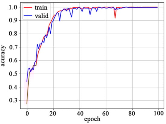
Figure 6.
Training accuracy and valid accuracy.
A detection model can be obtained by training the dataset. Test set is used to test the detection performance of the model, and the test result is shown in Table 3. The number of samples in the test set is 396. The recognition accuracy of “c0” is 100%, which is the highest. The recognition accuracy of “c6” is the lowest, at 92.2%. The average recognition accuracy of the four categories is 96.7%. The result showed that this method can identify single damage location accurately.
Table 3.
The test results.
In order to display the predicted results of the test set more intuitively, a visualization tool called “t-SNE” was employed to visualize the raw data and the output data of the convolutional neural network. “t-SNE” is a nonlinear dimensionality reduction technique, it is particularly well suited for the visualization of high-dimensional datasets. Thus, the raw data and the output data of CNN are displayed in two dimensions, as shown in Figure 7. The two-dimensional display of raw data is terrible. There is no distinction between the categories. However, the two-dimensional display of the output data of CNN is perfect. There is a clear distinction between the categories. The results showed that the proposed convolutional neural network has a powerful ability to extract features automatically.
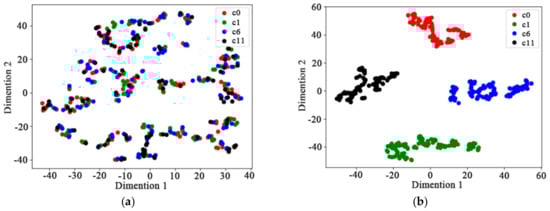
Figure 7.
The two-dimensional display of data. (a) raw data (b) output data of CNN.
4. Multiple Damage Location Detection
4.1. Multiple Damage Dataset
In the multiple damage location detection, stiffness of the damaged column was reduced by 20%. The multiple damage dataset includes five categories: “c0”, “c1c6”, “c1c11”, “c6c11”, and “c1c6c11”. “c0” means that there are no damaged columns; “c1c6” means that the damaged columns are column 1 and column 6; “c1c11” means that the damaged columns are column 1 and column 11; “c6c11” means that the damaged columns are column 6 and column 11; “c1c6c11” means that the damaged columns are column 1, column 6, and column 11. The data in the dataset were obtained from the finite element model. The specific parameters in the finite element model were set according to the damage types mentioned above. Displacement of each node in the finite element model under environmental excitation was collected. Meanwhile, the displacement of each node was converted into interlayer displacement, i.e., the interlayer displacement of 12 nodes was obtained. The acquisition frequency was set to 100 Hz. Each sample contains 50 data points, which is 0.5 s of acquisition time. Each sample in the dataset is a matrix of 12 × 50. Among them, 12 represents 12 nodes and 50 represents 50 data points. The number of samples is 399 in each category, and the dataset contains a total of 1995 samples. After these samples are randomly sorted, 1500 samples were used for training and verification, 495 samples were used as test set.
4.2. Detection Result
The training set and the valid set are inputted into the proposed convolutional neural network. Training accuracy and valid accuracy are shown in Figure 8. When the number of iteration epoch is 100, the training accuracy is 0.9900 and the valid accuracy is 0.9833. The detection accuracy has met the requirements of engineering.
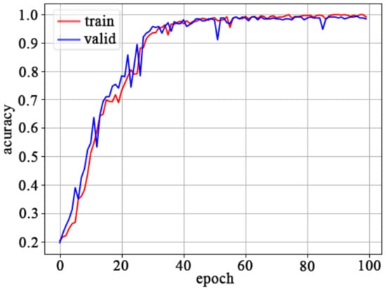
Figure 8.
Training accuracy and valid accuracy.
A detection model can be obtained by training the dataset. Test set is used to test the detection performance of the model, and the test result is shown in Table 4. The number of samples in the test set is 495. The recognition accuracies of “c0” and “c6c11” are 100%. The recognition accuracy of “c1c6c11” is 92.9%, 91 samples can be identified correctly, 4 samples can be misidentified as “c6c11”, and 3 samples can be misidentified as “c1c6”. The average recognition accuracy of the five categories is 97.36%. The result showed that this method can identify multiple damage locations accurately.
Table 4.
The test results.
The raw data and the output data of CNN are displayed in two dimensions, as shown in Figure 9. The two-dimensional display of raw data is also terrible. There is no distinction between the categories. However, the two-dimensional display of the output data of CNN is perfect. There is a clear distinction between the categories. It is not as effective as the two-dimensional display of single damage location detection; a small number of samples were misclassified. There are overlaps between different categories in the multiple damage location detection. For instance, “c1c6c11” means that the damaged columns are column 1, column 6, and column 11. Other categories overlap with “c1c6c11” partially. So, it is more difficult to distinguish. Nevertheless, the recognition accuracy of “c1c6c11” is 92.9%. The results showed that the proposed convolutional neural network has a powerful ability to detect multiple damage location.
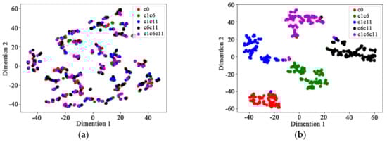
Figure 9.
The two-dimensional display of data. (a) raw data (b) output data of CNN.
5. Damage Degree Detection
5.1. Damage Degree Dataset
Section 3 and Section 4 both verify the effect of the structural damage location detection. This section verifies that the method still has a good recognition effect on the structural damage degree. Only column 1 was selected as the damaged column. In order to simulate different degrees of damage, the stiffness of the column 1 was reduced by 0, 10%, 20%, 30%, and 40%, respectively. The damage degree dataset includes five categories: “0”, “10%”, “20%”, “30%”, and “40%”. The number of samples is 399 in each category, and the dataset contains a total of 1995 samples. After these samples are randomly sorted, 1500 samples were used for training and verification, 495 samples were used as test set.
5.2. Detection Result
The training set and the valid set are inputted into the proposed convolutional neural network. Training accuracy and valid accuracy are shown in Figure 10. When the number of iteration epoch is 100, the training accuracy is 0.9642 and the valid accuracy is 0.9467. The detection accuracy has met the requirements of engineering.
Figure 10.
Training accuracy and valid accuracy.
A detection model can be obtained by training the dataset. The test set is used to test the detection performance of the model, and the test result is shown in Table 5. The number of samples in the test set is 495. The recognition accuracy of “0” is 100%. The recognition accuracy of “30%” is 84.3%, 70 samples can be identified correctly, 1 sample can be misidentified as “40%”, and 12 samples can be misidentified as “20%”. In addition, it can be found that the misidentified samples always are identified as adjacent categories. The difference between adjacent categories is very small, and it is difficult to distinguish them. However, the average recognition accuracy of the five categories is 97.36%. The result showed that this method can identify damage degree accurately.
Table 5.
The test results.
The raw data of the test set and the output data of the convolutional neural network are, respectively, displayed in two dimensions by “t-SNE”, as shown in Figure 11. The two-dimensional display of raw data is also terrible. There is no distinction between the categories. However, the two-dimensional display of the output data of CNN is perfect. There is a clear distinction between the categories. Because the difference between adjacent categories is very small, the misidentified samples always are identified as adjacent categories. In short, the proposed convolutional neural network can complete the damage degree detection.
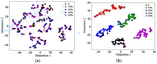
Figure 11.
The two-dimensional display of data. (a) raw data (b) output data of CNN.
6. Visualization of Convolutional Neural Networks
Convolutional neural networks have many hidden layers. The dataset is inputted into the CNN, and it automatically completes feature extraction and classification. However, the process of data processing in convolutional neural networks is confusing. In order to understand more intuitively how the convolutional neural networks work, the convolutional kernel and the outputs of some hidden layers are visualized.
6.1. Visualization of Convolutional Kernel
The convolutional kernel is one of the most important components in a convolutional layer. The initial parameters within the convolution kernel are randomly generated. These parameters are continually updated during the training process until the end of the training. The proposed convolutional neural network consists of two convolutional layers. The first convolutional layer has 32 convolution kernels of size 5 × 12. The second convolutional layer has 64 convolution kernels of size 5 × 32. The first two convolution kernels of the two convolutional layers are visualized. The visualization of the two convolution kernels in the first convolutional layer are shown in Figure 12. Each column of convolutional kernel is called the channel. The convolution kernel in the first convolutional layer has 12 channels. The curves of each channel are shown in Figure 13.
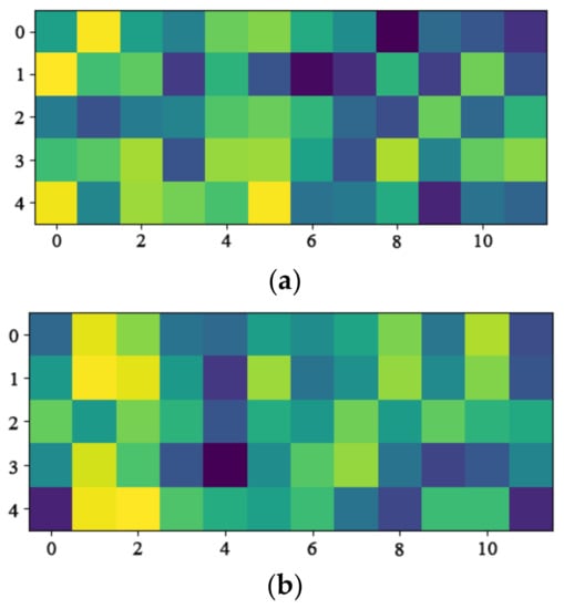
Figure 12.
The visualization of convolution kernels in the first convolutional layer. (a) Kernel 1 (b) Kernel 2.
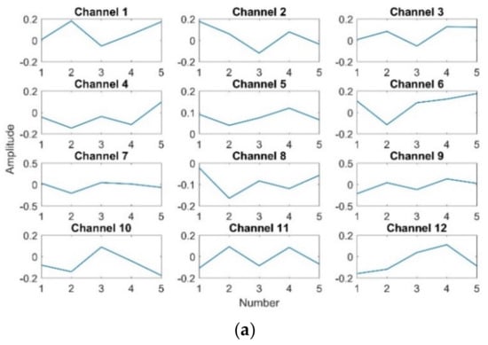
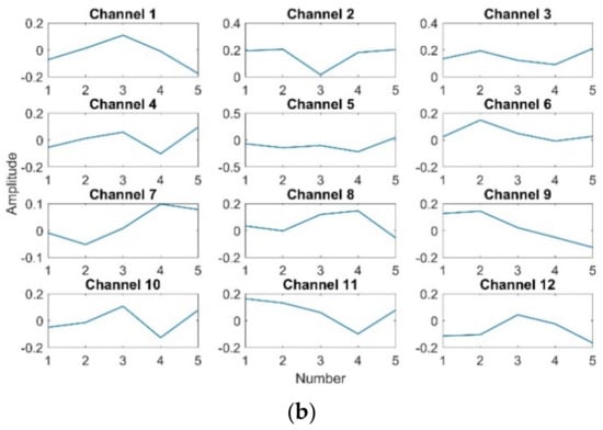
Figure 13.
The curve of each channel. (a) Kernel 1 (b) Kernel 2.
The visualizations of the two convolution kernels in the second convolutional layer are shown in Figure 14. Each column of convolutional kernel is called the channel. The convolution kernel in the second convolutional layer has 32 channels. The curves of the first twelve channels are shown in Figure 15.
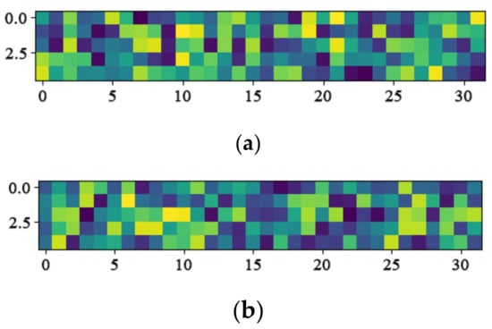
Figure 14.
The visualization of convolution kernels in the second convolutional layer. (a) Kernel 1 (b) Kernel 2.
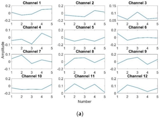
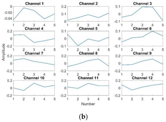
Figure 15.
The curve of the first twelve channels. (a) Kernel 1 (b) Kernel 2.
6.2. Visualization of the Outputs of Hidden Layers
In order to understand the process of CNN processing data, the input data, output of convolutional layer, output of pooling layer, and output of fully connected layer are visualized. In this section, the single damage test dataset is used as the input data. The shape of input data is 50 × 12. The data of each channel represent the interlayer displacement data of each node. The number of the data of each channel is 50, and the acquisition frequency is 100 Hz. The curves of each channel of the input data are shown in Figure 16. These curves are similar, and all have the characteristics of two cycles.
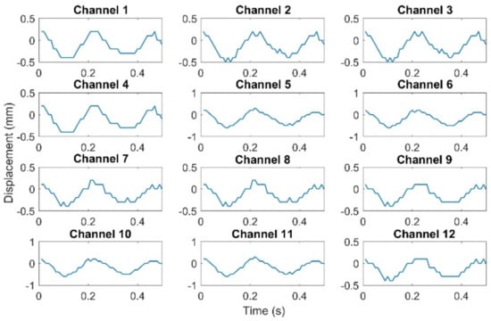
Figure 16.
Input data.
Convolution is the process of feature extraction in CNN, so the convolutional layer is also the most important part of the CNN. Taking the first convolutional layer as an example, the input shape is 50 × 12, the convolution kernel size is 5 × 12, and the number of the convolution kernel is 32. The output shape of the convolutional layer is 45 × 32, and each channel is generated by convolving the 12 channels of input data. The curves of the first twelve channels of output are shown in Figure 17. It can be seen that most of the twelve channels still maintain the characteristics of two cycles.
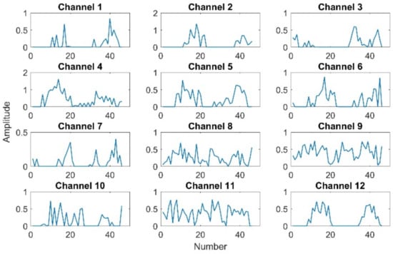
Figure 17.
Output of the first convolutional layer.
The role of the pooling layer is mainly to reduce the size of the feature map. Its input shape is 46 × 32, the pooling kernel size is 2 × 32, and the number of the pooling kernel is 32. Additionally, there are no parameters in the pooling kernel. The output shape of the pooling layer is 23 × 32. The curves of the first twelve channels of output are shown in Figure 18. The pooling layer reduces the size of the input data, but the outputs still maintain the shape and characteristics of the input data. At the same time, the curve becomes smoother. Thus, the pooling layer is similar to a filter.
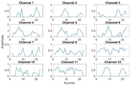
Figure 18.
Output of the first pooling layer.
After the second pooling layer, data are entered into the Flatten layer. The data are converted from a matrix to a vector. Then, the vector is inputted into the fully connected layer. The last fully connected (Dense) layer output the predicted probabilities of all sample. The probabilities of the first ten samples in single damage test dataset are shown in Table 6. As can be seen, each sample can be identified with high probability. The result showed that the model has a strong ability to detect structural damage.
Table 6.
Outputs of the second dense layer.
7. Conclusions
In this paper, a structure damage detection method based on one-dimensional convolutional neural network is proposed. The interlayer displacement of each node is collected under different damage states. The data are directly inputted into the proposed convolutional neural network, the data features are learned autonomously, and the damage detection result of the frame structure is outputted. Section 3 and Section 4 both verify the effect of the structural damage location detection. Section 5 verifies the effect of the damage degree detection. The results showed that the proposed method has high detection accuracy in all three types of damage detection. Furthermore, the method does not require feature extraction. The proposed method allows high-precision identification for various types of damage to building structures. However, it is difficult to build accurate finite element models in practical inspection. Therefore, further validation of the effect of the rough finite element model on damage identification is required. In addition, displacement is used as the input to the network in this paper. For large infrastructures where displacement is not easily detected, acceleration-based damage identification methods can be further considered. In the last section, the convolutional kernel and the outputs of some hidden layers are visualized to understand more intuitively how the convolutional neural networks work. Although the findings gained by studying convolutional neural networks are still unclear, visualization is the first step in understanding convolutional neural networks. In the future, the further research of the hidden layers of convolutional neural networks is required.
Author Contributions
The work presented here was carried out in collaboration between all authors. Z.X. contributed the conception of the proposed structure damage detection method. C.X. designed the three-layer framework model. Z.X. and D.W. analyzed the test data and prepared the manuscript. All authors have read and agreed to the published version of the manuscript.
Funding
This research was funded by the Science and Technology Plan Project of State Administration of Market Supervision (No. 2021MK044), the Basic Science (Natural Science) Project of Colleges and Universities in Jiangsu Province (No. 21KJB470031), and Science and Technology Plan Project of Jiangsu Market Supervision Administration (No. KJ196043).
Conflicts of Interest
The authors declare no conflict of interest.
References
- Chan, T.H.; Yu, L.; Tam, H.Y.; Ni, Y.Q.; Liu, S.Y.; Chung, W.H.; Cheng, L.K. Fiber Bragg grating sensors for structural health monitoring of Tsing Ma bridge: Background and experimental observation. Eng. Struct. 2006, 28, 648–659. [Google Scholar] [CrossRef]
- Jang, S.; Jo, H.; Cho, S.; Mechitov, K.; Rice, J.A.; Sim, S.-H.; Jung, H.-J.; Yun, C.-B.; Spencer, B.F., Jr.; Agha, G. Structural health monitoring of a cable-stayed bridge using smart sensor technology: Deployment and evaluation. Smart Struct. Syst. 2010, 6, 439–459. [Google Scholar] [CrossRef]
- Lee, S.-Y.; Lee, S.-R.; Kim, J.-T. Vibration-based structural health monitoring of harbor caisson structure. In Proceedings of the SPIE Smart Structures and Materials + Nondestructive Evaluation and Health Monitoring, San Diego, CA, USA, 6–10 March 2011; Volume 798154. [Google Scholar] [CrossRef]
- Yi, T.-H.; Li, H.-N.; Gu, M. A new method for optimal selection of sensor location on a high-rise building using simplified finite element model. Struct. Eng. Mech. 2011, 37, 671–684. [Google Scholar] [CrossRef]
- Yi, T.-H.; Li, H.-N.; Gu, M. Recent research and applications of GPS-based monitoring technology for high-rise structures. Struct. Control. Health Monit. 2012, 20, 649–670. [Google Scholar] [CrossRef]
- Park, J.-W.; Lee, J.-J.; Jung, H.-J.; Myung, H. Vision-based displacement measurement method for high-rise building structures using partitioning approach. NDT E Int. 2010, 43, 642–647. [Google Scholar] [CrossRef]
- Kammer, D.C. Sensor placement for on-orbit modal identification and correlation of large space structures. J. Guid. Control Dyn. 1991, 14, 251–259. [Google Scholar] [CrossRef]
- Ou, J.P.; Li, H. Structural Health Monitoring in mainland China: Review and Future Trends. Struct. Health Monit. 2010, 9, 219–231. [Google Scholar] [CrossRef]
- Salawu, O. Detection of structural damage through changes in frequency: A review. Eng. Struct. 1997, 19, 718–723. [Google Scholar] [CrossRef]
- Kim, J.-T.; Stubbs, N. Improved damage identification method based on modal information. J. Sound Vib. 2002, 252, 223–238. [Google Scholar] [CrossRef]
- Farrar, C.R.; Doebling, S.W. An overview of modal-based damage identification methods. In Proceedings of the DAMAS Conference, Sheffield, UK, 30 June–2 July 1997. [Google Scholar]
- Kim, J.-T.; Ryu, Y.-S.; Cho, H.-M.; Stubbs, N. Damage identification in beam-type structures: Frequency-based method vs mode-shape-based method. Eng. Struct. 2003, 25, 57–67. [Google Scholar] [CrossRef]
- Doebling, S.W. Minimum-rank optimal update of elemental stiffness parameters for structural damage identification. AIAA J. 1996, 34, 2615–2621. [Google Scholar] [CrossRef]
- Gao, Y.; Spencer, B.F.; Bernal, D. Experimental Verification of the Flexibility-Based Damage Locating Vector Method. J. Eng. Mech. 2007, 133, 1043–1049. [Google Scholar] [CrossRef]
- Stockwell, R. A basis for efficient representation of the S-transform. Digit. Signal Process. 2007, 17, 371–393. [Google Scholar] [CrossRef]
- Falkowski, M.J.; Smith, A.; Hudak, A.T.; Gessler, P.E.; Vierling, L.A.; Crookston, N.L. Automated estimation of individual conifer tree height and crown diameter via two-dimensional spatial wavelet analysis of lidar data. Can. J. Remote Sens. 2006, 32, 153–161. [Google Scholar] [CrossRef]
- Peng, Z.; Chu, F. Application of the wavelet transform in machine condition monitoring and fault diagnostics: A review with bibliography. Mech. Syst. Signal Process. 2004, 18, 199–221. [Google Scholar] [CrossRef]
- Sun, Z.; Chang, C.-C. Structural Damage Assessment Based on Wavelet Packet Transform. Eng. Struct. 2002, 128, 1354–1361. [Google Scholar] [CrossRef]
- Oh, C.K.; Sohn, H. Damage diagnosis under environmental and operational variations using unsupervised support vector machine. J. Sound Vib. 2009, 325, 224–239. [Google Scholar] [CrossRef]
- Widodo, A.; Kim, E.Y.; Son, J.-D.; Yang, B.-S.; Tan, A.C.; Gu, D.-S.; Choi, B.-K.; Mathew, J. Fault diagnosis of low speed bearing based on relevance vector machine and support vector machine. Expert Syst. Appl. 2009, 36, 7252–7261. [Google Scholar] [CrossRef]
- Tabrizi, A.; Garibaldi, L.; Fasana, A.; Marchesiello, S. Early damage detection of roller bearings using wavelet packet decomposition, ensemble empirical mode decomposition and support vector machine. Meccanica 2015, 50, 865–874. [Google Scholar] [CrossRef]
- Schölkopf, B.; Smola, A.J.; Williamson, R.C.; Bartlett, P.L. New Support Vector Algorithms. Neural Comput. 2000, 12, 1207–1245. [Google Scholar] [CrossRef]
- Zave, P. An experiment in feature engineering. In Programming Methodology; Springer: New York, NY, USA, 2003; pp. 353–377. [Google Scholar] [CrossRef]
- Xu, Y.; Hong, K.; Tsujii, J.; Chang, E.I. Feature engineering combined with machine learning and rule-based methods for structured information extraction from narrative clinical discharge summaries. J. Am. Med. Inform. Assoc. 2012, 19, 824–832. [Google Scholar] [CrossRef]
- Rumelhart, D.E.; Hinton, G.E.; Williams, R.J. Learning Internal Representations by Error Propagation; No. ICS-8506. California Univ San Diego La Jolla Inst for Cognitive Science; MIT Press: Cambridge, MA, USA, 1985. [Google Scholar]
- Lecun, Y.; Bottou, L.; Bengio, Y.; Haffner, P. Gradient-based learning applied to document recognition. Proc. IEEE 1998, 86, 2278–2324. [Google Scholar] [CrossRef]
- Hinton, G.E.; Salakhutdinov, R.R. Reducing the Dimensionality of Data with Neural Networks. Science 2006, 313, 504–507. [Google Scholar] [CrossRef]
- Krizhevsky, A.; Sutskever, I.; Hinton, G.E. Imagenet classification with deep convolutional neural networks. Commun. ACM 2017, 60, 84–90. [Google Scholar] [CrossRef]
- Zhang, Y.; Yuen, K. Crack detection using fusion features-based broad learning system and image processing. Comput. Civ. Infrastruct. Eng. 2021, 36, 1568–1584. [Google Scholar] [CrossRef]
- Zhang, Y.; Yuen, K.-V.; Mousavi, M.; Gandomi, A.H. Timber damage identification using dynamic broad network and ultrasonic signals. Eng. Struct. 2022, 263, 114418. [Google Scholar] [CrossRef]
- Zhang, Y.; Yuen, K.-V. Bolt damage identification based on orientation-aware center point estimation network. Struct. Health Monit. 2021, 21, 438–450. [Google Scholar] [CrossRef]
- Cha, Y.-J.; Choi, W.; Büyüköztürk, O. Deep Learning-Based Crack Damage Detection Using Convolutional Neural Networks. Comput. Civ. Infrastruct. Eng. 2017, 32, 361–378. [Google Scholar] [CrossRef]
- Zhang, Y.; Yuen, K.-V. Review of artificial intelligence-based bridge damage detection. Adv. Mech. Eng. 2022, 14, 16878132221122770. [Google Scholar] [CrossRef]
- Kocatepe, A.; Ulak, M.B.; Kakareko, G.; Ozguven, E.E.; Jung, S.; Arghandeh, R. Measuring the accessibility of critical facilities in the presence of hurricane-related roadway closures and an approach for predicting future roadway disruptions. Nat. Hazards 2018, 95, 615–635. [Google Scholar] [CrossRef]
- Kakareko, G.; Jung, S.; Ozguven, E.E. Estimation of tree failure consequences due to high winds using convolutional neural networks. Int. J. Remote Sens. 2020, 41, 9039–9063. [Google Scholar] [CrossRef]
- Amit, S.N.K.B.; Shiraishi, S.; Inoshita, T.; Aoki, Y. Analysis of satellite images for disaster detection. In Proceedings of the 2016 IEEE International geoscience and remote sensing symposium (IGARSS), Beijing, China, 10–15 July 2016; pp. 5189–5192. [Google Scholar]
- Zhao, K.; Kang, J.; Jung, J.; Sohn, G. Building extraction from satellite images using mask R-CNN with building boundary regularization. In Proceedings of the IEEE Computer Society Conference on Computer Vision and Pattern Recognition Workshops, Salt Lake City, UT, USA, 18–22 June 2018; Volume 2018, pp. 242–246. [Google Scholar]
- Cha, Y.-J.; Choi, W.; Suh, G.; Mahmoudkhani, S.; Büyüköztürk, O. Autonomous Structural Visual Inspection Using Region-Based Deep Learning for Detecting Multiple Damage Types. Comput. Civ. Infrastruct. Eng. 2017, 33, 731–747. [Google Scholar] [CrossRef]
- Cha, Y.-J.; Wang, Z. Unsupervised novelty detection–based structural damage localization using a density peaks-based fast clustering algorithm. Struct. Health Monit. 2017, 17, 313–324. [Google Scholar] [CrossRef]
- Wang, Z.; Cha, Y.-J. Unsupervised deep learning approach using a deep auto-encoder with a one-class support vector machine to detect damage. Struct. Health Monit. 2020, 20, 406–425. [Google Scholar] [CrossRef]
- Cha, Y.-J.; Chen, J.; Büyüköztürk, O. Output-only computer vision based damage detection using phase-based optical flow and unscented Kalman filters. Eng. Struct. 2017, 132, 300–313. [Google Scholar] [CrossRef]


Disclaimer/Publisher’s Note: The statements, opinions and data contained in all publications are solely those of the individual author(s) and contributor(s) and not of MDPI and/or the editor(s). MDPI and/or the editor(s) disclaim responsibility for any injury to people or property resulting from any ideas, methods, instructions or products referred to in the content. |
© 2022 by the authors. Licensee MDPI, Basel, Switzerland. This article is an open access article distributed under the terms and conditions of the Creative Commons Attribution (CC BY) license (https://creativecommons.org/licenses/by/4.0/).