A Machine Learning Approach for the Non-Destructive Estimation of Leaf Area in Medicinal Orchid Dendrobium nobile L.

Abstract

In this study, leaf area prediction models of Dendrobium nobile, were developed through machine learning (ML) techniques including multiple linear regression (MLR), support vector regression (SVR), gradient boosting regression (GBR), and artificial neural networks (ANNs). The best model was tested using the coefficient of determination (R²), mean absolute errors (MAEs), and root mean square errors (RMSEs) and statistically confirmed through average rank (AR). Leaf images were captured through a smartphone and ImageJ was used to calculate the length (L), width (W), and leaf area (LA). Three orders of L, W, and their combinations were taken for model building. Multicollinearity status was checked using Variance Inflation Factor (VIF) and Tolerance (T). A total of 80% of the dataset and the remaining 20% were used for training and validation, respectively. KFold (K = 10) cross-validation checked the model overfit. GBR (R², MAE and RMSE values ranged at 0.96, (0.82–0.91) and (1.10–1.11) cm²) in the testing phase was the best among the ML models. AR statistically confirms the outperformance of GBR, securing first rank and a frequency of 80% among the top ten ML models. Thus, GBR is the best model imparting its future utilization to estimate leaf area in D. nobile.

1. Introduction

Dendrobium nobile (Orchidaceae) is an endangered orchid species listed under Appendix II of CITES [1] and forms the largest vascular epiphytes having features of CAM plants [2]. It serves as an ornamental and medicinal food for humans [3]. Recently HPLC fingerprints showed a strong inhibiting effect on cancer cells, through increased bioactive compounds; signifying D. nobile as a functional herb for the market [4]. Leaf area is a necessary biometrical variable that helps not only in the computation of various physiological indices such as leaf area index (LAI), specific leaf area (SLA), net assimilation rate (NAR), specific leaf weight (SLW), leaf area duration (LAD) and various plant physiological mechanisms viz., photosynthesis, respiration, light interception, transpiration, etc. [5,6,7], but also water-related anatomical traits such as leaf density and vein density, thus, helping in water conservation and transport ultimately resulting in the ability of Dendrobium to cope in water stress situations in the environment [8]. Leaf area, shape, size, and number present per plant affects the source–sink relationship and ultimately the yield of the plant as green leaves act as a primary source of assimilates for petals in Dendrobium orchid [9,10]. Leaf area is also responsible for nutrient spray responsiveness in Dendrobium [11]. The leaf area trait, i.e., specific leaf area (SLA), is strongly influenced by phylogeny (k value > 1) indicating strong conservation in changes in this trait over evolution in Dendrobium [12]. Leaf area further can act as an important component of complex process-based plant growth models for the development of support decision-based systems for management of cultural practices in Dendrobium. Therefore, leaf area (LA) is a fundamental component of estimation of physiological, ecological, evolutionary, and anatomical traits that affect the survival, growth, and distribution of Dendrobium. Leaf area modeling enables an easy way of predicting LA through models which aid in a non-destructive estimation, rather than manual methods.

LA can be measured directly through techniques such as photographing [13], image analysis, blueprinting, use of expensive instruments including digital planimeter [14], scanning planimeter [15], etc. Major disadvantage in these direct methods lies in the removal of leaves, which poses a problem of not only for the experiments which are time-shared, but also leads to a decline in these valuable plant samples, in our case a rare and endangered orchid species. Other problems in these methods can be mentioned as requirements of time and labor, costly instruments, reduction in canopy affecting photosynthesis, growth, etc. The above bottleneck in LA estimation is successfully overcome through the various non-invasive technologies using very few measurements such as leaf length (L) and leaf width (W) or its different combination [16,17,18,19], constant leaf area term KA [20] or a correction factor [21]. These indirect LA estimation methods are performed in situ [22], low in cost, reliable, provide fast results without detachment of the leaves from the plants, and also excludes biological variations in the experiment [23]. In our study, an Orchidaceae family member, D. nobile, was assessed for LA estimation where conservation prioritization is essential and automated conservation assessments were recently performed through deep learning [24]; thus making it inevitable to use the non-destructive ML methods for development of LA prediction models.

Machine learning (ML) techniques have gained a lot of importance due to their non-requirement of explicit instructions, i.e., a data driven nature, and their reliable, non-destructive, fast, accurate, high throughput, user friendly and less laborious approach of solving real life problems. Recently, ML and modeling has become very popular in the field of LA estimation, as it allows the adjustments and improvements of the model for accurate prediction of LA in crops. The regression problem depicts the relationship between one continuous dependent variable and multiple independent variables. LA modeling in the present study underwent regression problem analysis as a continuous dependent variable leaf area (LA) was predicted by a numerical value using two independent variables leaf length (L) and leaf width (W). Multiple linear regression (MLR), the most common form of linear regression analysis, computes a weighted sum of the input features and a bias term, the intercept. Support vector regression (SVR) is a supervised ML algorithm to predict the dependent variable in the model. In principle, SVR is same as support vector machine (SVM) [25] which is capable of computing linear and non-linear regression problems. The gradient boosting regression (GBR) [26] algorithm is a decision tree-based ensemble technique for solving both linear and non-linear regression problems. The high flexibility to construct new base-learners which correlates maximally with the negative gradient of the loss function makes it a highly customizable data driven ML technique. Boosting algorithms are also very easy for various model design implementations, thus imparting gradient boosting machine applications in various fields of both practical and data mining and machine learning studies [27,28,29]. It is faster and has better model performance due to its principle of hypothesis boosting; the requirement of minimum data pre-processing has outperformed Artificial Neural Network (ANN) and SVM in many reports [30,31,32]. ANN techniques have been used in a limited number of crops which are summarized in the paper [33]. These models are self-adaptive, data driven, and non-linear in nature which helps to find the relationship between the predictor and predicted [34].

Performance metrices have been used for evaluation in multiple machine learning algorithms, but a unified and single standard metric is difficult to find. Another drawback of these metrices is since regression problem may have multiple values ranging from zero to infinity, merely a single metric cannot solve the problem of regression with respect to the ground truth elements in the study. Thus, in our study three performance evaluation metrices were used to assess the results of regression viz., coefficient of determination (R-squared or R² [35]) which determines the proportion of variance in the dependent variable which can be predicted from the independent variables; mean absolute error (MAE [36]) depicting the quality of fit in terms of the distance of the regressor to the actual training points; and Root mean Square Error (RMSE) for the detection of outliers [37]. We also used another statistical ranking method Average Rank (AR) that follows Friedman’s M statistic [38] to select the best model for Dendrobium orchid.

LA modeling has been reported for many crops including apple [39], walnut [13], apricot [40], onion [41], jatropha [42], cacao [43], cherry cultivars [14], chestnut [44], grapes [45,46], green and black peppers [33,47,48], ginger [49], medicinal and aromatic plants [50], niagara and grave vines [51], som [52], mango [53], tomato [54], cotton [55,56,57], multiple crops [58], kiwi fruit [59], durian [60], pecan [61], forest tree [62], and hazelnut [63]. Ornamentals received meagre attention; among them LA modeling was performed in zinnia [64], sunflower [65], rose [66], Euphorbia × lomi Thai hybrids [67], bedding plants [68], and bougainvillea [69]. The development of leaf dry weight and leaf area models in the four cultivars of Phalaenopsis orchids [70] was reported by considering the length and width of leaves and linear regression analysis, but a major limitation is the non-utilization of the progressively utilized ML techniques.

Advanced ML techniques to predict leaf area are reported in a very limited number of crops and the existing LA models are mostly based on linear regression analysis. Until now, no other attempts have been reported for non-destructive estimation of LA through ML techniques in the Orchidaceae family, which constitutes the second largest (c. 28,000) flowering family in the world; it is the most widespread and accounts for 8% of angiosperm species diversity [71]. Dendrobium, in this study for LA modeling, constitutes the largest genus of Orchidaceae, over 1800 species [72]. To the best of our knowledge, only a linear regression-based model (LRM) and recently very few works on neural net (NN)-based models have been reported for LA prediction. Our study reports for the first time a non-linear regression-based model, i.e., support vector regression (SVR) and decision tree-based ensemble model gradient boosting regression (GBR) for LA modeling and its robustness was compared with the state-of-the-art ML models and a novel method of statistical ranking of the LA models based on average rank (AR) was proposed. Keeping this in mind, the objectives of this study were set as to (i) determine the individual leaf length (L), width (W) and the leaf area (LA) using the ImageJ software [73], to ultimately develop a leaf area model from the nine input combinations of L and W using different ML techniques viz., MLR, SVR, GBR, and the nine best selected ANN models (ii) to evaluate the model robustness through various statistical performance metrices (R², MAE and RMSE) for selecting the best LA prediction model and (iii) to rank the ML models based on average rank (AR) ranking methodology in the orchid D. nobile.

2. Materials and Methods

2.1. Plant Material

The present study was conducted in the glass house located at ICAR-National Research Centre for Orchids (ICAR-NRCO), Pakyong, Sikkim, India (27.2267° N, 88.5877° E). The individual leaf images were collected from D. nobile orchid from 1.5 to 2 years of age. A mixture of stone or brick pieces, leaf mold, coconut husks, and semi rotten logs in the ratio of 1:1:1:1 in plastic pots of (5 to 6) inches was used as the potting media of D. nobile. The N:P:K composition as 20:10:10 @ 0.5% was sprayed on the 1 to 2 year old plants and potting materials at an interval of 15 days and other nutrients such as calcium nitrate @ 0.05%, iron sulphate @ 50 ppm, magnesium sulphate @ 0.1%, boric acid @ 50 ppm and zinc sulphate @ 50 ppm were sprayed at 60 days interval. Neem @ 3% and copper oxychloride @ 0.3% were sprayed once every fortnight for controlling sucking pests and foliar diseases, respectively. The number of average leaves in the plant was approximately 10 and image was captured by a smartphone (Samsung Galaxy J7 with 13 MP camera, resolution of 4128 × 3096 pixels, autofocus, and LED flash) during 10:30 a.m. to 3:30 p.m. from July to August of 2020. The light intensity was recorded by lux meter (LutronLX-101A, Delhi, India) every day at 12:00 p.m. regardless of the weather or cloud cover over the 4 weeks experimental period. The glass house ambient light intensity varied from 531 lux to 1413 lux. Direct bright sunlight was avoided by providing a green colored shade net of 50% over the glass house (Saveer Biotech Ltd., New Delhi, India). Ambient day and night temperature ranged to about 32 °C and 17 °C during the photoperiod and relative humidity varied from 60 to 80% inside the glass house.

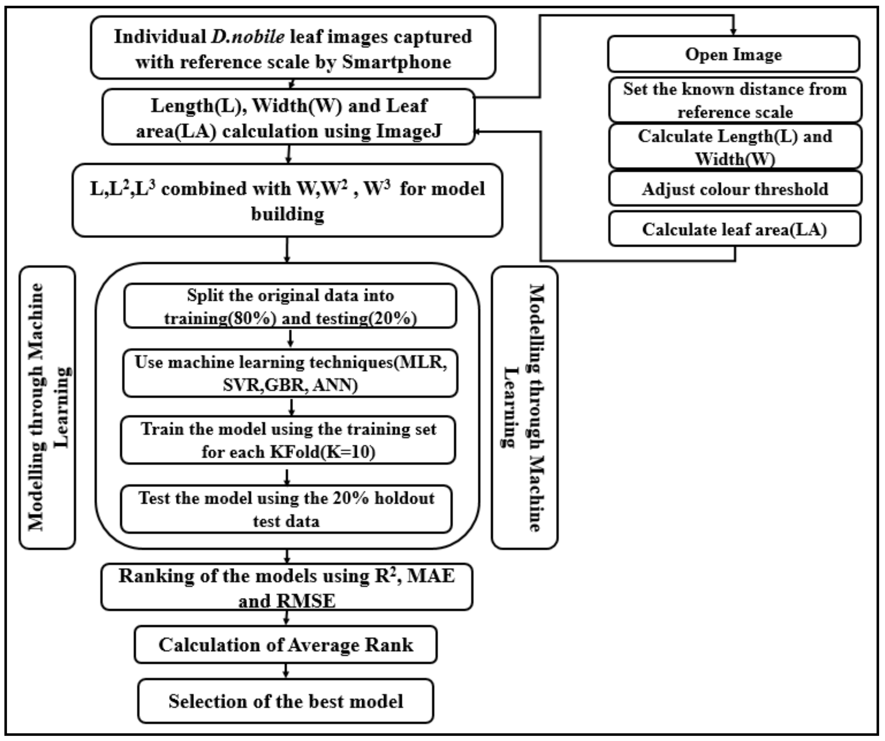
2.2. Process Flow of Selection of Best Leaf Area Model in D. nobile through ML Techniques

Figure 1 depicts the whole workflow of the study conducted for the non-destructive estimation of leaf area using ML. Firstly, the individual leaves of the D. nobile were captured with a reference scale by a smartphone (Figure 2). Then the ImageJ (https://imagej.nih.gov/ij/ (accessed on 27 April 2020)) software was used for determining the individual leaf length (L), width (W), and the leaf area (LA) of D. nobile. Three orders of independent variable viz., first order, second order, and third order polynomial functions of L and W were taken which can be denoted as L, L², and L³ and W, W², and W³, respectively. L, L², and L³ were combined with W, W², and W³, respectively, thus totalling to the number of input combinations as 3 × 3, i.e., 9. These nine combinations of inputs were used for MLR, SVR, and GBR machine learning techniques for model building. For ANN, we used four types of architectures and considered the nine combinations of L and W, the total number of models were 4 × 9 = 36. Finally, the nine best ANN models were selected based on R², MAE, and RMSE values. Thus, the above nine models from each of MLR, SVR, GBR, and ANN were compared together with their respective performance metrices. For the study, the original dataset was split into 80% training and 20% testing dataset for model development and its validation. To avoid the over fitting of the ML model KFold (k = 10) cross-validation [74] was performed using cross_val_score on the training dataset. The rest of the 20% holdout data were used for testing of the model. R², MAE, and RMSE were used for ranking of the models. Selection of the best leaf area model was performed through higher R² values and lower MAE and RMSE values. Lastly, AR was used to statistically confirm the best performing models through ranks.

2.3. Dataset

A total of 1589 D. nobile leaf images were collected by Samsung Galaxy J7 smartphone for the study. The image was captured with a reference scale and the ImageJ software was used for estimation of the length, width, and area of the individual leaf [75]. The color threshold function of ImageJ was used to demarcate the captured leaf area from its background, thus automatically calculating the region of interest, i.e., measured leaf area (LA). The dataset contains one continuous dependent variable, i.e., leaf area (LA) and two independent variables—leaf length (L) and leaf width (W). The measurement of the leaf length (L) was taken from the tip of the lamina to the intersection point between the leaf and petiole. The leaf width (W) measurement was taken from end-to-end point between the broadest part of the lamina exactly perpendicular to the midrib of D. nobile lamina. All the variables were measured in cm scale. The values of three variables, length (L), width (W), and leaf area (LA) were stored in csv format for further model development processing and submitted to the dataset repository Mendeley data [http://doi.org/10.17632/8tk2sc4ytg.1 (published on 28 June 2021)] and KRISHI, ICAR research data repository for knowledge management [http://krishi.icar.gov.in/jspui/handle/123456789/71908 (published on 6 May 2022)] (Supplementary S1).

Table 1. Input combinations of L, W, and their variants with model names of MLR, SVR, and GBR.

Inputs	W	W2	W3
L	L, W (MLR1, SVR1, GBR1)	L, W2 (MLR2, SVR2, GBR2)	L, W3 (MLR3, SVR3, GBR3)
L2	L2, W (MLR4, SVR4, GBR4)	L2, W2 (MLR5, SVR5, GBR5)	L2, W3 (MLR6, SVR6, GBR6)
L3	L3, W (MLR7, SVR7, GBR7)	L3, W2 (MLR8, SVR8, GBR8)	L3, W3 (MLR9, SVR9, GBR9)

depicts the different combination of inputs of L and W along with their ML models. In this experiment three orders of L and W were taken, so L, L², and L³ were combined with W, W², and W³. Each L and its higher order were combined with W and its higher order. The total number of input combination thus can be calculated as 3 × 3, i.e., 9. These nine combinations of inputs were used for MLR, SVR, and GBR techniques. The higher orders of L and W were taken to observe their effect on model building. For ANN, four types of architectures were designed and the total number of models were 4 × 9 = 36. Finally, the nine best ANN models were selected based on R², MAE, and RMSE values (Figure 3 and

Table 2. Combination of different inputs for ANN techniques with different ANN architectures.

Models	Input Variables	Output Variable	Layers (Input-Hidden-Output)
ANN1	L, W	LA	2-3-1
ANN2	L, W	LA	2-5-1
ANN3	L, W	LA	2-10-1
ANN4	L, W	LA	2-3-3-1
ANN5	L, W2	LA	2-3-1
ANN6	L, W2	LA	2-5-1
ANN7	L, W2	LA	2-10-1
ANN8	L, W2	LA	2-3-3-1
ANN9	L, W3	LA	2-3-1
ANN10	L, W3	LA	2-5-1
ANN11	L, W3	LA	2-10-1
ANN12	L, W3	LA	2-3-3-1
ANN13	L2,W	LA	2-3-1
ANN14	L2,W	LA	2-5-1
ANN15	L2,W	LA	2-10-1
ANN16	L2,W	LA	2-3-3-1
ANN17	L2, W2	LA	2-3-1
ANN18	L2, W2	LA	2-5-1
ANN19	L2, W2	LA	2-10-1
ANN20	L2, W2	LA	2-3-3-1
ANN21	L2, W3	LA	2-3-1
ANN22	L2, W3	LA	2-5-1
ANN23	L2, W3	LA	2-10-1
ANN24	L2, W3	LA	2-3-3-1
ANN25	L3, W	LA	2-3-1
ANN26	L3, W	LA	2-5-1
ANN27	L3, W	LA	2-10-1
ANN28	L3, W	LA	2-3-3-1
ANN29	L3, W2	LA	2-3-1
ANN30	L3, W2	LA	2-5-1
ANN31	L3, W2	LA	2-10-1
ANN32	L3, W2	LA	2-3-3-1
ANN33	L3, W3	LA	2-3-1
ANN34	L3, W3	LA	2-5-1
ANN35	L3, W3	LA	2-10-1
ANN36	L3, W3	LA	2-3-3-1

).

2.4. ML Methodologies Used for LA Prediction Modeling

2.4.1. Multiple Linear Regression Analysis (MLR) Models

Multiple linear regression (MLR) is a variant of simple linear regression with more than one explanatory or independent variable. It can capture linear relationships between independent variables and the dependent variable. It performs better in the absence of multicollinearity within the dependent variables and dependent and independent should be linearly correlated with each other [76]. The equation for MLR model estimation is as follows [77]:

$$\mathrm{y}={\mathsf{\beta }}_0+{\mathsf{\beta }}_1{\mathrm{x}}_1+\dots +{\mathsf{\beta }}_2{\mathrm{x}}_2+\dots +{\mathsf{\beta }}_{\mathrm{k}}{\mathrm{x}}_{\mathrm{k}}+ϵ$$

(1)

where y is the dependent variable (LA), x_i is the ith independent variable (L or W), β_i is the polynomial coefficients of x_i, k is the number of independent variables, and ε is the possible variation form.

2.4.2. Support Vector Regression (SVR) Models

SVR is based on the Vapnik–Chervonenkis (VC) theory which in principle is structural risk minimization [78] and is an effective tool for estimating real-valued functions [79]. The advantages of SVR, which was harnessed in this study, is its highly effective performance for both the linear and non-linear regression dataset and not too large dataset which results in the use of Gaussian RBF kernel hyperparameter (for non-linear regression) thus mapping each training instance to an infinite-dimensional space [80]. The other usefulness of SVR can be summarized as its excellent capability of generalization with high accuracy prediction. Default hyperparameters used in sklearn.svm.SVR are kernel = ‘rbf’, degree = 3, gamma = ‘scale’, coef0 = 0.0, tol = 0.001, C = 1.0, epsilon = 0.1, shrinking = True, cache_size = 200, verbose = False, and max_iter = −1.

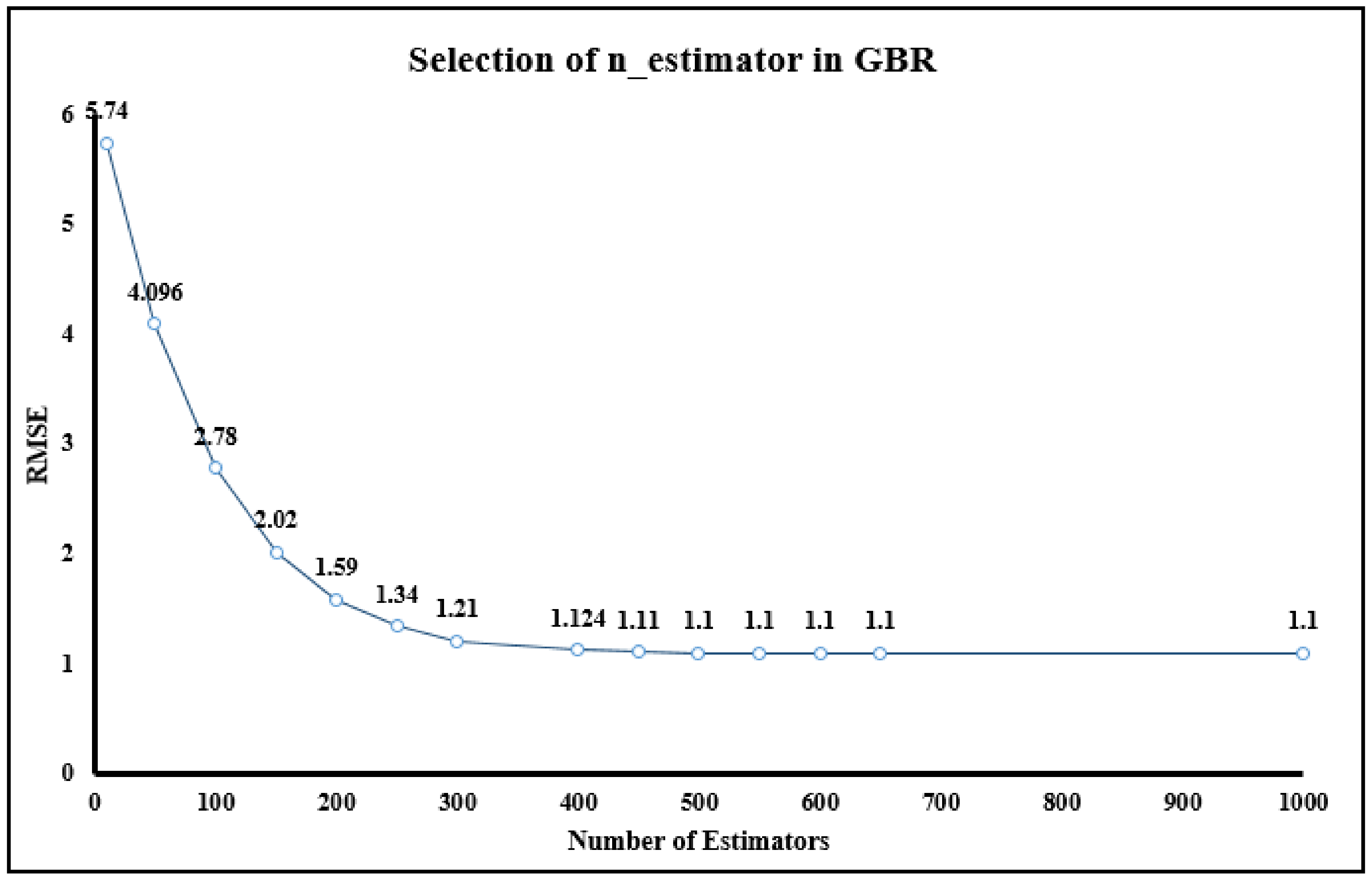
2.4.3. Gradient Boosting Regression (GBR) Models

GBR develops an additive model that serially adds predictors or new base learners to an ensemble and each one corrects its predecessors leading to the minimization of the loss function. In each iterative training process, the residual value in the current model denotes the negative gradient of the loss function, and a new regression tree (predictor) is trained to fit the current residual and added subsequently to the previous model. For developing a GBM model, both the loss function and the function corresponding to the negative gradient must be specified. In our study, loss function for continuous response viz., least-square was used which usually neglects smaller deviations but refits larger ones. One of the advantages of GB models is that it provides the flexibility to use a variety of base learning models at the same time for designing a complex model for a particular solution. A model’s regularization capability is of the utmost importance for model building from data because it prevents the overfit of the data [81]. Our study used shrinkage as a regularization technique which reduces unstable regression coefficients by shrinking it to zero which is normally used in ridge regression problems. The hyperparameters used in our study were n_estimators to control the ensemble training through the number of boosted trees to fit the training data; min_samples and max_depth to control the growth of decision trees; and learning rate to scale the contribution of each tree via a regularization technique known as shrinkage, the lower the value the better the generalization of the predictions will be. The value of the learning rate and n_estimator were adjusted in our experiment to 0.01 and 500, respectively, which performed better than the other combinations tried. The loss hyperparameter controls the cost function of GBR.

Table 3. Descriptions of hyperparameters tuned in GBR and ANN models.

GBR			ANN
Hyper Parameters	Values	Descriptions	Hyper Parameters	Values	Descriptions
n_estimators	500	No of decision tree in the ensemble	alpha	0.001	Regularization parameter
max_depth	4	Maximum depth of the decision tree	hidden_layer_sizes	(3,); (5,); (10,); (3,3)	Four architecture 2-3-1, 2-5-1, 2-10-1, 2-3-3-1
min_samples_split	5	Minimum number if sample required to split an internal node	max_iter	1000	No. of iteration
learning_rate	0.01	Determine the impact of each tree on final outcome.	activation	‘logistic’	Logistic sigmoid function $\frac{1}{\left(1+ex{p}^{-x}\right)}$
loss	‘ls’	Least square loss function	learning_rate	‘adaptive’	Keep learning rate constant as the initial learning rate

depicts the hyperparameters, their values and descriptions which were adjusted to improve the learning performances in GBR and ANN.

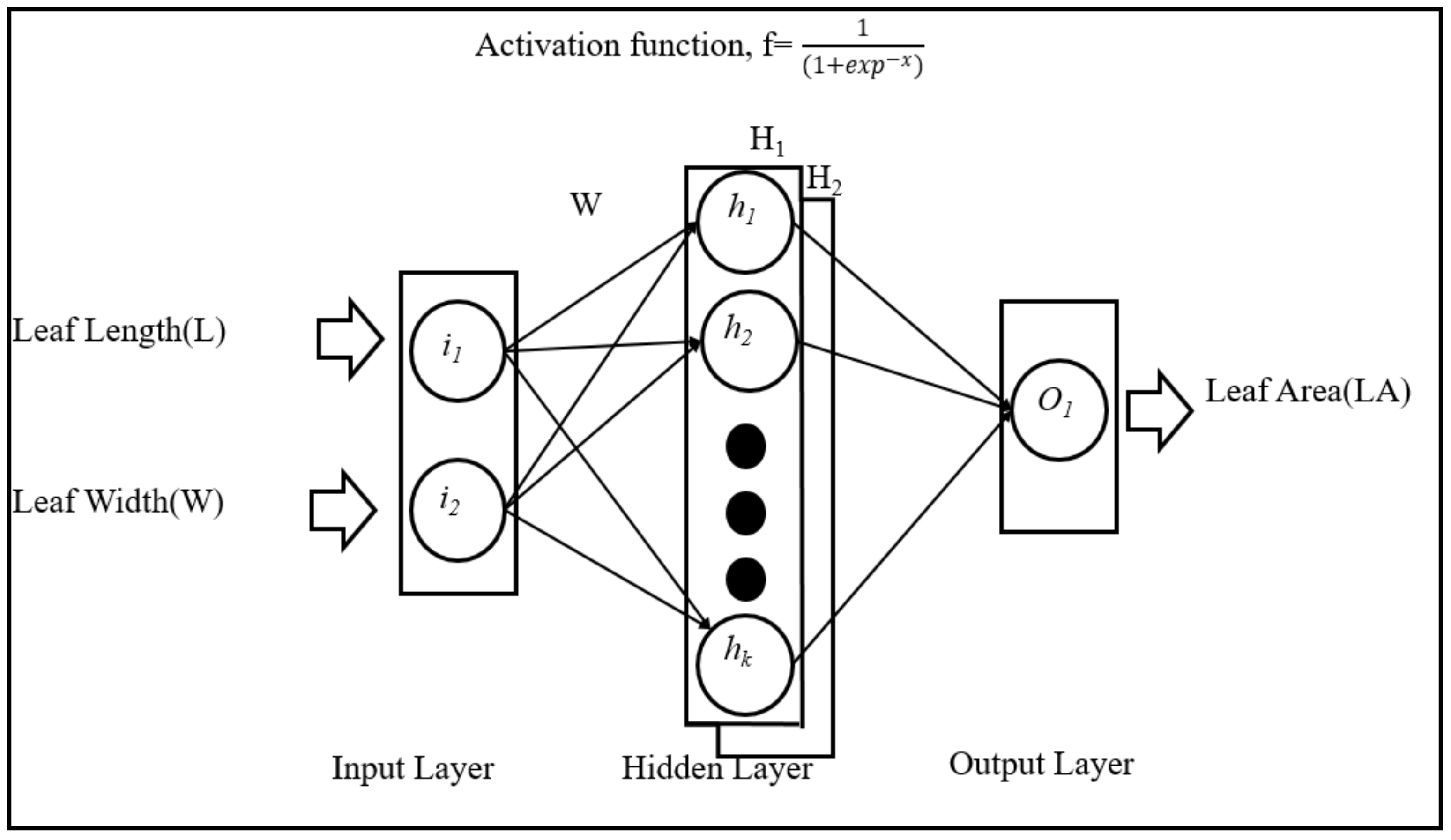
2.4.4. Artificial Neural Networks (ANNs) Models

ANNs are data-driven, non-linear, and self-adaptive techniques capable of establishing a relationship between the input data and target output data even when they have an unknown relationship [82]. The mathematical structures of ANN models have a resemblance with the neural system of the human brain [78]. They process data collectively through interconnected neurons depending on factors including thresholds, adjustable weights, and mathematical transformation functions of the images [83]. The ANN architecture used in our study comprised of three layers, where the input and output layers depict the independent and dependent variables, and the hidden layer (inter layer) deals with the computation of data and establishes interconnection between the input and output layers through the hidden neurons. The optimum neurons in the hidden layer were determined through the trial and error approach [84]. In our study, a single hidden layer was found to provide better accuracy than the double hidden layers which is in accordance with the literature [61]. Figure 3 and Table 2 depict the different ANN models where nine types of inputs (as described in Table 1) were combined with four types of ANN architectures, i.e., input layer-hidden layer-output layer (2-3-1, 2-5-1, 2-10-1, 2-3-3-1) in total calculating to 4 × 9 = 36 models of ANN. This was performed to observe the effects of different hidden layers on ANN models leading to the selection of the nine best models based on the coefficient of determination (R²), mean absolute errors (MAEs), and root mean square errors (RMSEs) values of the testing phase.

The learning rate was adaptive in nature, i.e., constant as the initial learning rate (0.001) as long as the training loss decreased and number of iterations were determined as 1000 epochs for convergence. To capture the non-linearity of the data an activation function, sigmoid, was used. The hyperparameters, their values and descriptions used for ANN model building are described in Table 3.

2.5. Feature Correlation Heatmap and Multicollinearity of the Independent Variables

A feature correlation heatmap of L, W, and its variants (L², L³, W², and W³) and LA was generated through the matplotlib package of Python library. Pairwise Pearson’s correlation coefficient, r [85] in the seaborn heatmap functions from seaborn module of Python was applied among the different combination of variables. The Variance Inflation Factor (VIF) and Tolerance values (T) were calculated to check the multicollinearity status of the two independent variables (L and W) and their variants (L², L³, W², and W³). VIF values >10 or T value <0.10 denote the effect of multicollinearity on the estimation of the parameters of the model that lead to its non-reliability and for that problem at least one of the independent variables must be excluded from the prediction model [86].

The equations of Pairwise Pearson’s correlation coefficient (r) and Variance Inflation Factor (VIF) [87] and Tolerance (T) [88] are shown below:

$$\mathrm{r}=\frac{{{\displaystyle \sum }}_{\mathrm{i}}^{\mathrm{n}}\left({\mathrm{x}}_{\mathrm{i}}-\overline{\mathrm{x}}\right)\left({\mathrm{y}}_{\mathrm{i}}-\overline{\mathrm{y}}\right)}{{{\displaystyle \sum }}_{\mathrm{i}}^{\mathrm{n}}{({\mathrm{x}}_{\mathrm{i}}-\overline{\mathrm{x}})}^2{\left({\mathrm{y}}_{\mathrm{i}}-\overline{\mathrm{y}}\right)}^2}$$

(2)

where n = number of data points; i varies from 1 to n; x and y are two independent variables; $\overline{\mathrm{x}}$ and $\overline{\mathrm{y}}$ are means of x and y, respectively.

$$\mathrm{VIF}=\frac{1}{\left(1-{\mathrm{r}}^2\right)}$$

(3)

r is the correlation coefficient.

$$\mathrm{T}=\frac{1}{\mathrm{VIF}}$$

(4)

2.6. Programming Set-Up

The experiment was conducted on an HP Omen laptop computer with i7 9th generation processor (8 GB RAM, 4 GB GEFORCE GTX nVIDIA GPU, 1 TB HDD, 250 GB SSD Windows 10 operating system). The experiments were conducted in Pycharm Community Edition 2020.2 IDE using Python 3.7 version. For our study, we used many python packages including numpy, pandas, sklearn, matplotlib, etc.

Linear regression of sklearn.linear_model, SVR of sklearn.svm, gradient boosting regressor of ensemble, and MLP regressor of sklearn.neural_network modules available in sklearn were used for implementation of MLR, SVR, GBR, and ANN ML techniques respectively. Training and testing was performed using train_test_split methods of sklearn.model_selection, mean_squared_error, mean_absolute_error, and r2_score of sklearn.metrics were used for calculation of the performance of the machine learning algorithm [89].

The equations are defined as under [77]:

$${\mathrm{R}}^2=\frac{{{\displaystyle \sum }}_{\mathrm{i}=1}^{\mathrm{n}}\left({\mathrm{LA}}_{\mathrm{mea}}-{\overline{\mathrm{LA}}}_{\mathrm{mea}}\right)\left({\mathrm{LA}}_{\mathrm{mea}}-{\overline{\mathrm{LA}}}_{\mathrm{est}}\right)}{{{\displaystyle \sum }}_{\mathrm{i}=1}^{\mathrm{n}}{\left({\mathrm{LA}}_{\mathrm{mea}}-{\overline{\mathrm{LA}}}_{\mathrm{mea}}\right)}^2{{\displaystyle \sum }}_{\mathrm{i}=1}^{\mathrm{n}}{\left({\mathrm{LA}}_{\mathrm{mea}}-{\overline{\mathrm{LA}}}_{\mathrm{est}}\right)}^2}$$

(5)

$$\mathrm{MAE}=\frac{{{\displaystyle \sum }}_{\mathrm{i}=1}^{\mathrm{n}}\left|\left.{\mathrm{LA}}_{\mathrm{mea}}-{\overline{\mathrm{LA}}}_{\mathrm{est}}\right|\right.}{\mathrm{n}}$$

(6)

$$\mathrm{RMSE}=\sqrt{\frac{{{\displaystyle \sum }}_{\mathrm{i}=1}^{\mathrm{n}}{\left({\mathrm{LA}}_{\mathrm{mea}}-{\overline{\mathrm{LA}}}_{\mathrm{est}}\right)}^2}{\mathrm{n}}}$$

(7)

where LA_mea = measured LA value; LA_est = estimated LA value; (${\overline{\mathrm{LA}}}_{\mathrm{mea}}$) = average values of measured LA value; (${\overline{\mathrm{LA}}}_{\mathrm{est}}$) = average values of estimated LA value; n = number of leaves used for training or testing phase.

2.7. Model Performance Evaluation

A model evaluation is an essential step in machine learning problems. Several methods are available in literature to evaluate machine learning methods. The statistical model performance criteria used in this study were: coefficient of determination (R²), mean absolute errors (MAEs), and root mean square errors (RMSEs).

In general, R², MAE, or RMSE cannot predict the departure patterns of observed values in the study against the predicted values. In the scatter plot an overlap of the reference line (y = x) and regression line of observed vs. predicted values were visualized. Departures of the regression line of observed vs. predicted values from the reference line suggests an over or underestimation [90].

2.8. Model Ranking Based on Average Rank (AR) Ranking Methodology

For each 36 ML models which includes the four ML techniques viz., MLR, SVR, GBR, and ANN, based on the performance metrices R², MAE, and RMSE, ranks were assigned. The best algorithm was ranked as first (1st) and second best as second (2nd) and so on, both for the testing as well as training phase, so each model obtains six ranks, three from training (R², MAE and RMSE) and three from testing (R², MAE and RMSE). The average ranks were obtained by averaging the ranks for each model. The final rank was derived by arranging the average ranks in an ascending order.

The formula for the calculation of average rank (AR) is as follows [38]:

$${\mathrm{AR}}_{{\mathrm{model}}_{\mathrm{j}}}=\frac{{{\displaystyle \sum }}_{\mathrm{i}=1}^6{\mathrm{r}}_{\mathrm{i}}}{6}$$

(8)

where j varies from 1 to 36 for 36 ML models, r_i represents the ith rank of a model, i varies from 1 to 6

3. Results and Discussion

The LA prediction modeling study presented here is of importance to the physiologists, horticulturalist, and environmentalist as D. nobile is a rare and endangered epiphytic medicinal orchid listed officially in the Pharmacopoeia of the People’s Republic of China (Chinese Pharmacopoeia Commission, 2015) for the Dendrobine content as an active ingredient category [91]. The low reproduction rate in the wild, slow growth, and poor regeneration ability may prove D. nobile to be vulnerable under the predicted scenario of climate change as suggested by MaxEnt ML models that their habitat will shrink from (1–10)% in the future [92]. Leaf area (LA) estimation is of the utmost importance for performing any physiological experiments investigating the growth characteristics for studying the impact of predicted climate change.

First, the descriptive statistics of D. nobile leaves was calculated, next feature correlation heatmap and multicollinearity status of the variables was assessed. A selection of nine best performing ANN models based on R², MAE, and RMSE was tested. Finally, a comparison of state-of-the-art ML models for estimating leaf area of D. nobile leaves based on R², MAE, and RMSE was addressed and ranking of the models was performed statistically based on Average Rank (AR) ranking methodology.

3.1. Descriptive Statistics of D. nobile Leaves Used for LA Model Building

The descriptive statistics was studied and summarized in

Table 4. Descriptive statistics of D. nobile leaves.

Parameters	Maximum	Minimum	Mean and Standard Deviation
Leaf Length (L) cm	16.30	5.24	10.68 and 1.57
Leaf Width (W) cm	4.34	1.30	2.39 and 0.51
Leaf Area (LA) cm2	43.90	6.39	20.04 and 6.26

where maximum length, minimum length, width, and leaf area as well as mean and standard deviation of those parameters of D. nobile leaves were described. Sampling of leaves for image capture was performed to cover a wide range of leaf sizes. Leaf length (L) ranged from 5.24 cm to 16.30 cm with the mean of 10.68 and standard deviation of 1.57. Width (W) ranged from 1.30 cm to 4.34 cm with the mean of 2.39 and standard deviation of 0.51. Leaf area (LA) ranged from 6.39 cm² to 43.902 cm² with the mean of 20.042 cm and standard deviation of 6.26.

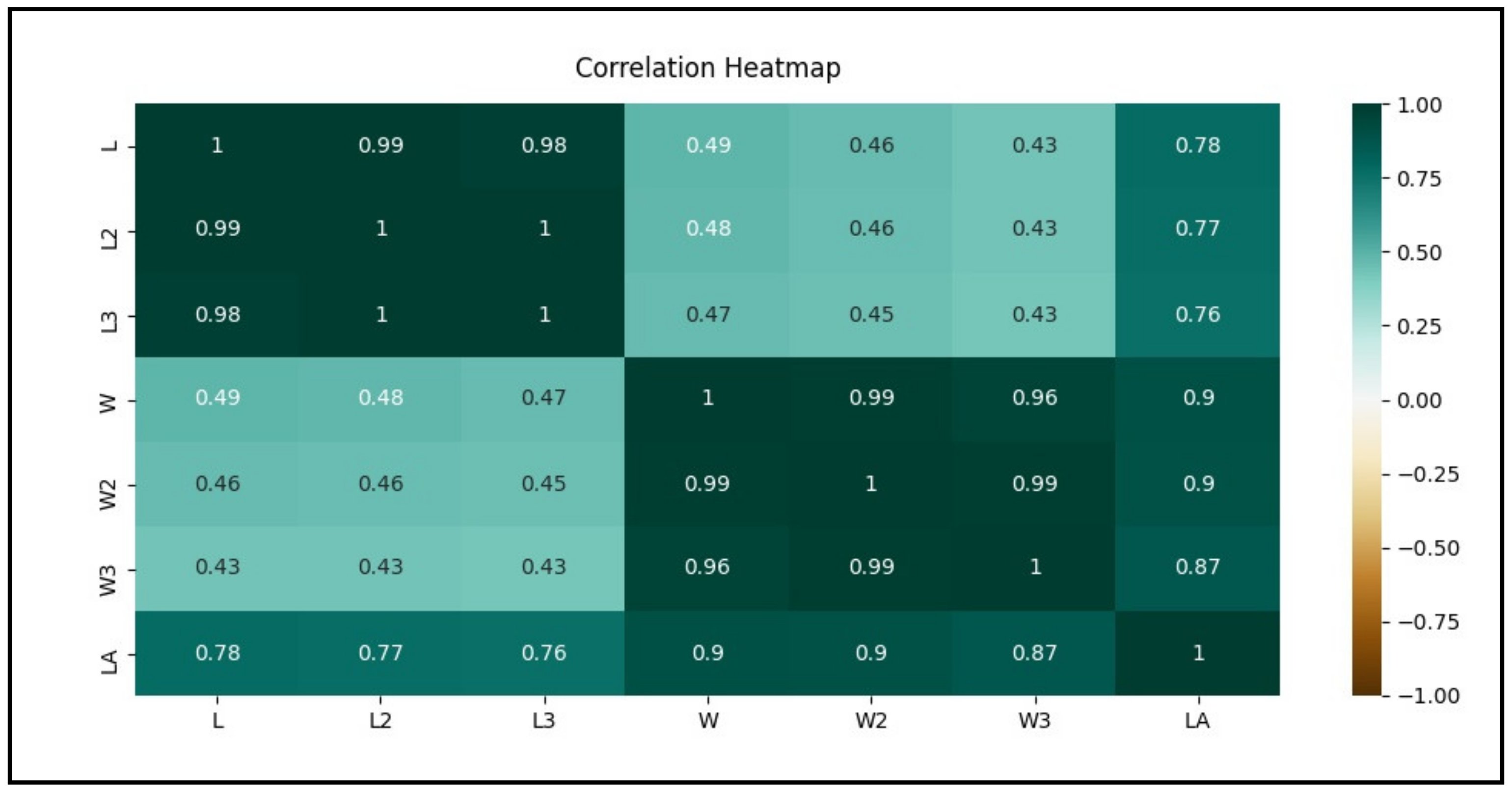
3.2. Feature Correlation Heatmap between the Variables through Correlation Coefficient

The correlation heatmap illustrating the relationship between each variable and compared with every other variable is depicted in Figure 4. The following observations can be made from the heatmap generated for the two independent variables (L, L², L³, W, W², W³) and LA in our study:

• Leaf length (L) and width (W) are linearly least correlated (r = 0.43–0.49) to each other as depicted from the light green color;
• L, L², L³, and LA are nearly equally correlated (r = 0.76–0.78) to each other as depicted from the medium green color;
• Leaf width (W) shows more correlated to leaf area (LA) with correlation coefficient (r) values ranging between 0.87 and 0.9 than leaf length (L) 0.76–0.78 as depicted from the darker green color in the heatmap;
• Among the variants of leaf width, the best to worst correlation with the leaf area (LA) can be shown in the order of W (r = 0.9) = W² (r = 0.9) > W³(r = 0.87);
• L, W, and their variants are strongly linearly correlated with leaf area (LA) where r ranges from 0.76 to 0.90 as depicted from dark green color in the heatmap.

3.3. Multicollinearity Status of the Two Independent Variables (L and W)

In our study, the VIF ranged from (1.22 to 1.31) and T ranged from (0.76 to 0.82) for independent variables L, W, and their variants (

Table 5. The values of VIF and T of L, W, and their input combinations.

Methods	Input Combinations
	L, W	L, W2	L, W3	L2, W	L2, W2	L2, W3	L3, W	L3, W2	L3, W3
Variance Inflation Factor (VIF)	1.31	1.27	1.23	1.30	1.27	1.23	1.28	1.25	1.22
Tolerance (T)	0.76	0.78	0.81	0.77	0.79	0.81	0.78	0.80	0.82

) which are less than the non-acceptable VIF values, i.e., >10 and higher than T value < 0.10 to state the effect of multicollinearity on the estimation of the parameters of the model. Thus, the independent variables and the variants can provide accurate and reliable model building results overcoming the effects of multicollinearity.

3.4. Selection of Nine Best Performing ANN Models Based on R², MAE and RMSE

From 36 models of ANN, nine models were selected based on nine different input combinations as mentioned in Table 2. One best model was selected from every input combination. ANN1–ANN4 came under the LW combination of inputs. ANN2 showed the highest R² value (0.96) and lowest MAE (0.86) and RMSE (1.13 cm²) in the testing phase. ANN5–ANN8 came under the LW² combination of inputs. ANN6 showed highest R² value (0.96) and lowest MAE (0.84) and RMSE (1.18 cm²) in the testing phase. ANN9–ANN12 came under LW³ combination of inputs. ANN10 showed highest R² value (0.97) and lowest MAE (0.87) and RMSE (1.18 cm²) in the testing phase. ANN13-ANN16 came under L²W combination of inputs. ANN15 showed highest R² value (0.97) and lowest MAE (0.86) and RMSE (1.11 cm²) in the testing phase. ANN17–ANN20 came under the L²W² combination of inputs. ANN18 shows the highest R² value (0.96) and lowest MAE (0.77) and RMSE (1.11 cm²) in the testing phase. ANN21–ANN24 came under the L²W³ combination of inputs. ANN22 showed the highest R² value (0.97) and lowest MAE (0.86) and RMSE (1.19 cm²) in the testing phase. ANN25–ANN28 came under the L³W combination of inputs. ANN26 showed the highest R² value (0.88) and lowest MAE (1.35) and RMSE (2.06 cm²) in the testing phase. ANN29–ANN32 came under the L³W² combination of inputs. ANN31 showed the highest R² value (0.94) and lowest MAE (1.01) and RMSE (1.47 cm²) in the testing phase. ANN33–ANN36 came under the L³W² combination of inputs. ANN35 showed the highest R² value (0.96) and lowest MAE (0.97) and RMSE (1.31 cm²) in the testing phase. Finally, the selected nine best performing ANN models which were to be compared with the other three models viz., MLR, SVR, and GBR includes ANN2, ANN6, ANN10, ANN15, ANN18, ANN22, ANN26, ANN31, and ANN35.

Table 6. Comparative analysis of 36 ANN models with different inputs, i.e., LW, LW², LW³, L²W, L²W², L²W³, L³W, L³W², L³W³ for selection of 9 best models for each input combinations based on the statistical performance metrices (R², MAE and RMSE) of models.

Inputs	Model	Training			Testing
		R2	MAE	RMSE (cm2)	R2	MAE	RMSE (cm2)
LW	ANN1	0.96	0.93	1.29	0.96	0.89	1.21
LW	ANN2	0.96	0.87	1.27	0.96	0.86	1.13
LW	ANN3	0.96	0.86	1.26	0.96	0.93	1.32
LW	ANN4	0.85	1.03	2.51	0.96	0.98	1.32
LW2	ANN5	0.96	0.96	1.30	0.96	0.88	1.23
LW2	ANN6	0.96	0.90	1.25	0.96	0.84	1.18
LW2	ANN7	0.96	0.91	1.28	0.96	0.84	1.21
LW2	ANN8	0.93	1.13	1.50	0.94	1.18	1.62
LW3	ANN9	0.96	0.92	1.28	0.95	0.91	1.35
LW3	ANN10	0.96	0.90	1.27	0.97	0.87	1.18
LW3	ANN11	0.96	0.90	1.23	0.96	0.91	1.29
LW3	ANN12	0.95	1.12	1.63	0.96	0.88	1.20
L2W	ANN13	0.94	1.00	1.55	0.94	1.12	1.60
L2W	ANN14	0.95	0.96	1.48	0.96	0.92	1.40
L2W	ANN15	0.95	0.94	1.41	0.97	0.86	1.11
L2W	ANN16	0.92	2.28	5.17	0.95	1.07	1.45
L2W2	ANN17	0.95	1.00	1.44	0.96	0.91	1.34
L2W2	ANN18	0.94	0.93	1.36	0.97	0.77	1.11
L2W2	ANN19	0.95	0.94	1.39	0.96	0.89	1.24
L2W2	ANN20	0.74	1.60	4.05	0.00	4.62	5.84
L2W3	ANN21	0.94	1.03	1.47	0.95	0.88	1.32
L2W3	ANN22	0.95	0.97	1.39	0.97	0.86	1.19
L2W3	ANN23	0.95	0.90	1.32	0.96	0.92	1.34
L2W3	ANN24	0.83	1.67	3.19	0.95	0.93	1.26
L3W	ANN25	0.47	2.73	3.74	0.88	1.42	2.06
L3W	ANN26	0.73	2.77	3.78	0.88	1.35	2.06
L3W	ANN27	0.70	2.46	4.32	0.88	1.38	2.17
L3W	ANN28	0.39	3.19	4.41	0.83	1.61	2.68
L3W2	ANN29	0.86	1.63	3.46	0.93	1.07	1.61
L3W2	ANN30	0.81	1.36	2.15	0.89	1.13	1.97
L3W2	ANN31	0.88	1.41	2.22	0.94	1.01	1.47
L3W2	ANN32	0.75	1.90	3.02	0.88	1.54	2.06
L3W3	ANN33	0.87	2.04	2.32	0.85	1.58	2.45
L3W3	ANN34	0.77	1.57	2.54	0.86	1.41	2.38
L3W3	ANN35	0.88	1.29	2.34	0.96	0.97	1.31
L3W3	ANN36	0.85	1.92	3.58	0.89	1.38	1.99

enumerates the performance metrices (R², MAE, and RMSE) of 36 ANN models.

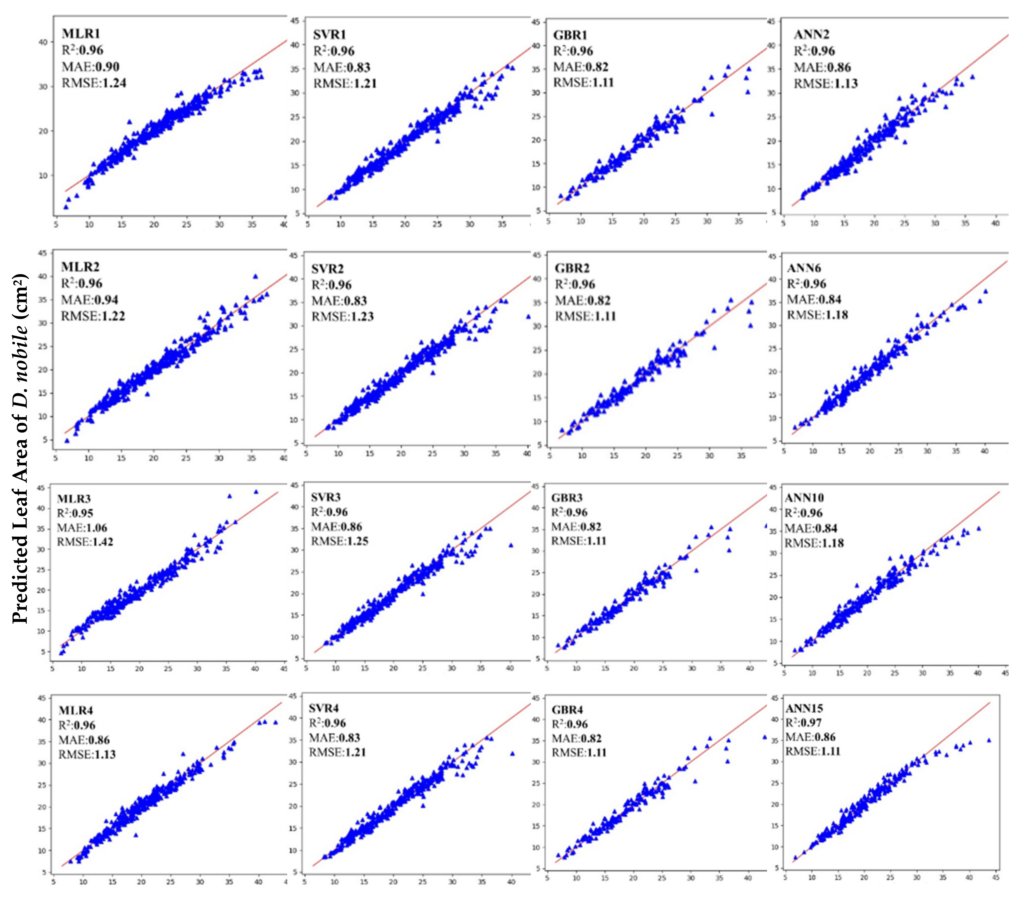
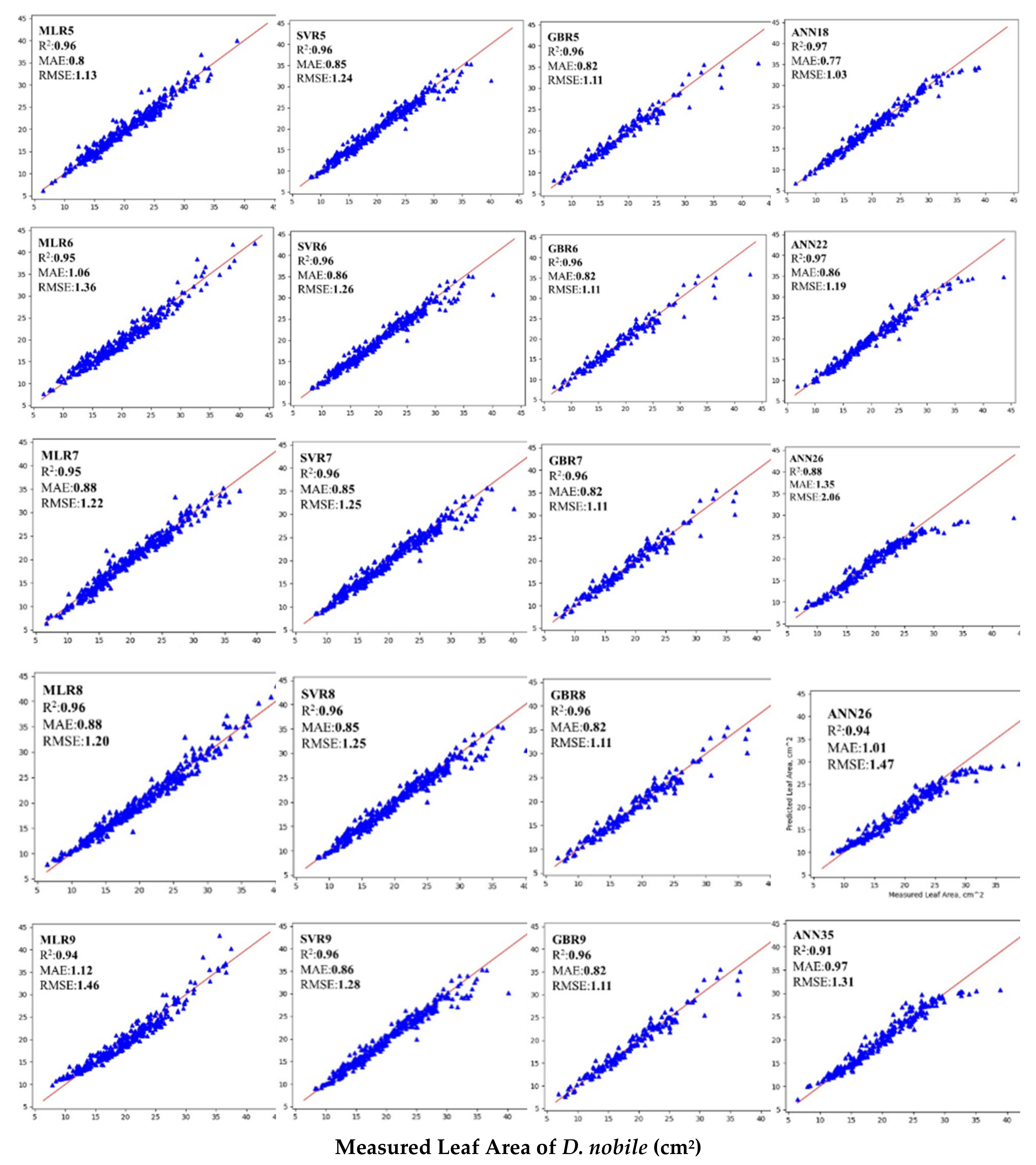
3.5. Comparisons of Different ML Models for Estimating Leaf Area of D. nobile Leaves

A sum of 63 different ML models was developed for estimating the LA of D. nobile leaves. Input combinations are described in Table 1, which forms the various ML models: MLR (1–9), SVR (1–9), and GBR (1–9), each has nine models using the various input combinations. ANN also used these input combinations along with different network architectures which are described in Table 2. Among the 36 ANN models (Table 6) developed for each input combination, the best nine ANN models were taken based on higher R² and lower MAE and RMSE values. Therefore, for LW, LW², LW³, L²W, L²W², L²W³, L³W, L³W², and L³W³ input combinations ANN2 (2-5-1), ANN6 (2-5-1), ANN10 (2-5-1), ANN15(2-10-1), ANN18 (2-5-1), ANN22 (2-5-1), ANN26 (2-5-1), ANN31 (2-10-1), and ANN35 (2-10-1) models, respectively, were compared with other models, i.e., MLR, SVR, and GBR.

Table 7. Developed LA models for three orders of L and W input combinations of D. nobile leaves using MLR techniques.

Model Input Combinations	Models
MLR1	LA = −18.72 + L × 1.74 + W × 8.41
MLR2	LA = −9.01 + L × 1.79 + W2 × 1.65
MLR3	LA = −6.76 + L × 1.92 + W3 × 0.40
MLR4	LA = −9.56 + L2 × 0.08 + W2 × 8.34
MLR5	LA = 0.28 + L2 × 0.75 + W2 × 0.98
MLR6	LA = 3.37 + L2 × 0.089 + W3 × 0.40
MLR7	LA = −6.6 + L3 × 0.00049 + W × 8.45
MLR8	LA = 3.5 + L × 1.79 + W2 × 1.65
MLR9	LA = 6.8 + L3 × 0.0054 + W3 × 0.40

depicts the LA models developed using different input combinations of L and W of D. nobile leaves using MLR (MLR1-MLR9) machine learning techniques.

A comparison of the performance statistics of MLR, SVR, GBR, and ANN models used for LA estimation was performed based on testing and training results using R², MAE, and RMSE values which are enumerated in

Table 8. Comparative statistical performance analysis of MLR, SVR, GBR, and ANN with different inputs, i.e., LW, LW², LW³, L²W, L²W², L²W³, L³W, L³W², L³W³ studied for LA estimation of D. nobile.

Inputs	Model	Training			Testing
		R2	MAE	RMSE (cm2)	R2	MAE	RMSE (cm2)
LW	ANN2	0.96	0.87	1.27	0.96	0.86	1.13
LW	GBR1	0.96	0.86	1.18	0.96	0.82	1.11
LW	SVR1	0.94	0.87	1.47	0.96	0.83	1.21
LW	MLR1	0.96	0.90	1.2	0.96	0.9	1.24
LW2	ANN6	0.96	0.90	1.25	0.96	0.84	1.18
LW2	GBR2	0.96	0.86	1.18	0.96	0.82	1.11
LW2	SVR2	0.94	0.89	1.52	0.96	0.84	1.23
LW2	MLR2	0.97	0.87	1.15	0.96	0.94	1.22
LW3	ANN10	0.96	0.90	1.27	0.97	0.87	1.18
LW3	GBR3	0.96	0.86	1.18	0.96	0.82	1.11
LW3	SVR3	0.94	0.93	1.58	0.96	0.86	1.25
LW3	MLR3	0.95	1.05	1.34	0.95	1.06	1.42
L2W	ANN15	0.95	0.94	1.41	0.97	0.86	1.11
L2W	GBR4	0.96	0.86	1.18	0.96	0.82	1.10
L2W	SVR4	0.94	0.88	1.48	0.96	0.83	1.21
L2W	MLR4	0.96	0.86	1.15	0.96	0.86	1.13
L2W2	ANN18	0.95	0.93	1.36	0.97	0.77	1.03
L2W2	GBR5	0.96	0.86	1.18	0.96	0.82	1.10
L2W2	SVR5	0.94	0.89	1.53	0.96	0.85	1.24
L2W2	MLR5	0.97	0.84	1.16	0.96	0.85	1.13
L2W3	ANN22	0.95	0.97	1.39	0.97	0.86	1.19
L2W3	GBR6	0.96	0.86	1.18	0.96	0.82	1.10
L2W3	SVR6	0.94	0.92	1.57	0.96	0.86	1.26
L2W3	MLR6	0.95	1.04	1.36	0.95	1.06	1.36
L3W	ANN26	0.73	2.77	3.78	0.88	1.35	2.06
L3W	GBR7	0.96	0.86	1.18	0.96	0.82	1.10
L3W	SVR7	0.94	0.88	1.49	0.96	0.85	1.25
L3W	MLR7	0.96	0.89	1.17	0.95	0.88	1.22
L3W2	ANN31	0.88	1.41	2.22	0.94	1.01	1.47
L3W2	GBR8	0.96	0.86	1.18	0.96	0.91	1.10
L3W2	SVR8	0.94	0.89	1.53	0.96	0.85	1.26
L3W2	MLR8	0.96	0.88	1.17	0.96	0.88	1.2
L3W3	ANN35	0.91	1.29	2.34	0.91	0.97	1.31
L3W3	GBR9	0.96	0.86	1.18	0.96	0.91	1.10
L3W3	SVR9	0.94	0.92	1.56	0.96	0.86	1.28
L3W3	MLR9	0.95	1.11	1.42	0.94	1.12	1.46

. The R² value in the training phase varied from (0.95–0.97), 0.94, 0.96, and (0.73–0.96) in case of MLR, SVR, GBR, and ANN, respectively. Similarly, the MAE values in the training phase varied from (0.84–1.11), (0.87–0.93), 0.86 and (0.87–2.77), for MLR, SVR, GBR, and ANN, respectively. RMSE values in the training phase ranged from (1.15–1.42) cm², (1.47–1.58) cm², 1.18 cm² and (1.25–3.78) cm², for MLR, SVR, GBR, and ANN, respectively. In the testing phase, the R² values ranged from (0.94–0.96), 0.96, 0.96, and (0.88–0.97) for MLR, SVR, GBR, and ANN, respectively. Similarly, the MAE values in the testing phase varied from (0.85–1.12), (0.83–0.86), 0.82 and (0.77–1.35), for MLR, SVR, GBR, and ANN, respectively. RMSE values ranged from (1.13–1.46) cm², (1.21–1.28) cm², 1.11 cm² and (1.03–2.06) cm², for MLR, SVR, GBR, and ANN, respectively. It was observed in our study that R², MAE, and RMSE values among the different input combinations in the training as well as in the testing dataset in GBR models showed nearly indifferent performance values. GBR showed a stable high R² values and low MAE and RMSE values in the dataset studied (Table 8) and outperformed other ML methods studied as also evident from the AR ranking methodology (

Table 9. Comparative statistical performance analysis of MLR, SVR, ANN, and GBR based on average rank (AR) ranking methodology.

Models	Ranks Based on Training Results			Ranks Based on Testing Results			Average Rank (AR)	Final Rank
	R2	MAE	RMSE (cm2)	R2	MAE	RMSE (cm2)
GBR7	7	4	8	11	2	2	5.67	1
MLR5	1	1	3	7	13	12	6.17	2
GBR6	8	5	9	12	3	3	6.67	3
GBR5	9	6	10	13	4	4	7.67	4
GBR4	11	8	11	14	5	5	9.00	5
GBR9	3	2	6	9	28	6	9.00	6
MLR4	10	7	1	5	19	13	9.17	7
GBR8	5	3	7	10	29	7	10.17	8
GBR3	12	9	12	15	6	8	10.33	9
GBR2	14	10	13	16	7	9	11.50	10
ANN18	22	27	20	2	1	1	12.17	11
MLR2	2	12	2	6	30	22	12.33	12
MLR8	4	15	4	8	25	18	12.33	13
GBR1	17	11	14	17	8	10	12.83	14
ANN10	13	22	18	1	24	16	15.67	15
ANN6	15	23	16	19	11	15	16.50	16
ANN2	18	13	17	20	20	14	17.00	17
MLR7	6	18	5	30	26	21	17.67	18
ANN15	23	29	23	4	18	11	18.00	19
ANN22	21	30	22	3	17	17	18.33	20
SVR1	33	14	25	21	9	19	20.17	21
MLR1	16	24	15	18	27	25	20.83	22
SVR4	30	17	26	22	10	20	20.83	23
SVR7	27	16	27	23	14	26	22.17	24
SVR2	32	21	28	24	12	23	23.33	25
SVR8	26	19	29	25	15	28	23.67	26
SVR5	29	20	30	26	16	24	24.17	27
SVR9	25	25	31	27	21	30	26.50	28
SVR6	28	26	32	28	22	29	27.50	29
MLR6	20	31	21	32	34	32	28.33	30
SVR3	31	28	33	29	23	27	28.50	31
MLR3	24	32	19	31	33	33	28.67	32
MLR9	19	33	24	33	35	34	29.67	33
ANN35	34	34	35	35	31	31	33.33	34
ANN31	35	35	34	34	32	35	34.17	35
ANN26	36	36	36	36	36	36	36.00	36

). This can be attributed due to GBR models ensembling individual models which can have characteristics of being both weak and overfitting nature but the final ensembled model leads to overcome these problems, also it requires lower data pre-processing leading to low error of prediction and high stability [93,94]. No reports of GBR for LA prediction modeling in plants is known to date. However, the outperformance of GBR over other ML methods are noticed in other fields. A recent study reported that gradient boosting regression algorithm (GBR) and random forest (RF) was employed for predicting and analyzing the net ecosystem carbon exchange (NEE) at UK-Gri, based on the flux data and meteorological data. GBR outperformed three state-of-the-art ML regression prediction models viz., stochastic gradient descent, support vector machine, and Bayesian ridge as GBR allows to tune a sufficient number of hyperparameters [31]. Another study depicted a model built on the gradient boosting regression tree (GBRT) with a limited sample size of data for predicting complex battery dynamics and its lifespan; having many extracted features was shown to outperform other ML algorithms. They suggested the hyperparameters viz., learning rate, maximum number of splits, and number of trees as the key to such performance. A 5-fold cross-validation technique was also applied to GBRT to prevent overfit [32]. Similar tuning of the hyperparameters (n_estimator, maximum_depth, min_sample split and learning rate) and a 10-fold cross-validation technique were applied in our leaf area modeling study and may have resulted in the best performance of GBR in our study. Again, an experiment was performed for predicting the return temperature over other ML models of district heating systems in Tianjin, China on a decision tree-based ensemble algorithm gradient boosting (GB) and it can be seen that GB outperforms other ML models without the requirement of complex feature transformation and they highlighted the importance of n_estimator in lowering the RMSE values of the tree-based model GB and RF [95]. A plot of RMSE of GBR with n_estimator tuned for our study is drawn in Figure 5. In our study RMSE equals to 2.78 when n_estimator is 100 and there is a decreasing trend upon increment of the n_estimator. RMSE is reduced to around 1.21 and 1.12 when n_estimator is 300 and 400, respectively. Eventually, the RMSE stabilizes to 1.1 at n_estimator 500 and achieves asymptote until it reaches 1000. This revealed the general principle that an improvement in the performance of the serial framework-based model, i.e., GBR model may be achieved (through decreased RMSE) upon increasing the n_estimator number [95]. Similarly, another report supporting GBR performance over other ML methods revealed that gradient boosting models achieved the best performance outperforming random forest and SVM for identifying the relation extraction of medications to the adverse effects of drugs, [96]. A recent report on the outperformance of GBR over ANN can be seen in the prediction of risk analysis of offshore platform integrity for its subsequent use or reuse for alternative energy applications. They studied the effect of stressors on the Remaining Useful Life (RUL). The performance metrices in the study viz., R², MAE, MSE, and RMSE depicted a slightly higher value of R² for GBR and a lower value for MAE, MSE, and RMSE than ANN model [30]. The results of these studies on the recent literatures were in general agreement of our observation highlighting our result of the best performance of GBR models in LA prediction in D. nobile orchid over the three ML models MLR, SVR, and ANN.

In our study, it can be seen that within the 10 best models MLR5 and MLR4 secured second and seventh position, respectively, based on AR ranking methodology (Table 9). Suitability criteria of MLR to produce good prediction accuracy are dependent on the factors which include the absence of multicollinearity between the predictors (measured by VIF and T), strong linear correlation between the predictors and dependent variable, and finally imposing the cross-validation methodology to prevent the over fit of the models. The results depicted from VIF and T values of our experiment show that L, W, and their variants are linearly independent to each other, i.e., there is an absence of multicollinearity. From the feature correlation heatmap it can be inferred that L, W, and their variants are strongly linearly correlated with leaf area (LA) where r ranges from 0.76 to 0.90. The 10-fold cross-validation was also performed to prevent overfitting of the models. Although the MLR model for LA prediction in previous studies did not outperform ANN or other decision tree-based models, there are reports in other fields in agreement with our results of outperformance over ANN and other complex models. A study by [97] showed MLR outperformed random forest based on the VIF values and cross-validation techniques for predicting Soil Organic Carbon stocks. Similar results were seen in another report [98] of the outperformance of MLR over other more complex modeling approaches. The reports of better prediction performance of MLR over ANN were further inferred by [99].

Previous studies on leaf area modeling by [34,47,54,60,100,101] depicted that ANN outperformed MLR. On the contrary, in our study ANN could not perform better in other input combinations than MLR as well as GBR except in L²W² input combinations of testing results where, ANN18 with (2-5-10) architecture secured a rank of eleventh based on AR ranking (Table 9) (R² = 0.97, MAE = 0.77 and RMSE = 1.03), which may be due to its inherent disadvantages such as overfitting. The reason behind this abrupt performance is due to the observed training results of ANN18, which shows R² = 0.95, MAE = 0.93, and RMSE = 1.36 denoting an overfit. The problems of local minima as well as selection of suitable hyper-parameters suitable for our study may be the other causes of such results of ANN18 [102].

From Table 9 It can be seen that SVR occupied ranks between twenty-first to thirty-first among the 36 models. So, it can be inferred that SVR was unable to perform better than three other ML models tested in our dataset.

For evaluating the prediction quality, a scatter plot of predicted LA and measured LA values along with the reference line (y = x) of D. nobile for the four ML models viz., MLR, SVR, GBR, and ANN in the testing period was used (Figure 6). A deviation of the regression line of predicted LA and measured LA values from the reference line is suggestive of a bias. In our study, the model showing the least bias was gradient boosting regression (GBR). Thus, it can be depicted that GBR models have a better capacity to predict LA in D. nobile than other ML models used. ANN and SVR models showed maximum deviations from the measured leaf area for all the input combinations studied.

The main limitations of performance metrices viz., R², MAE, and RMSE metrices as seen in our study is that if algorithm A outperforms B based on only r², then again it takes down A and brings up B on the basis of either MAE or RMSE. This is in accordance with the theorem of No Free Lunch (NFL) and the solution depends on the domain of the problem and knowledge of algorithms by the analysts [103,104]. Thus, ranking of the algorithms by average rank (AR) was chosen, whereby for each 36 ML models which includes the four ML techniques viz., MLR, SVR, GBR, and ANN ranks were assigned based on R², MAE, and RMSE. The average ranks were obtained by averaging the ranks for each model. The final rank was derived by arranging the average ranks in ascending order. Table 9 depicts a comparative statistical analysis of MLR, SVR, ANN, and GBR algorithms and assigned ranks on R², MAE, and RMSE each based on the training results and testing results to calculate the average rank. The final rank depicted that GBR7 secured the first rank among the 36 models as well as GBR algorithm has a frequency of occurrence of nearly 80% among the top 10 ML models. This provided a conclusive decision to select GBR as the best model for leaf area predictive modeling in the case of the Dendrobium orchid. Subsequent to the GBR algorithm, MLR occupied nearly 20% frequency among the top 10 ML models. Figure 7 depicts the frequency of the occurrence of the ML models studied in our experiment among the top ten ranks. It can be seen from the graph that GBR occupies 80% and MLR occupies 20% among the top ten ranks. On the other hand, SVR and ANN occupy nil percentage in the proposed rank group.

Light interception by the plant is totally dependent on the two-dimensional structure viz., length (L) and width (W) [105] and thus highlighting the importance of only those two proxy variables [13,40,62,87,106,107,108,109]. In this study, a non-destructive methodology of LA modeling in D. nobile through ML techniques was proposed that can be employed to develop a web portal or mobile app for providing an interactive user interface to obtain rapid, precise, and accurate leaf area estimation results from simple measurements such as leaf length (L) and leaf width (W). The proposed best model, i.e., GBR can play a crucial role in real time LA estimation of D. nobile avoiding the need for expensive instruments and destructive sampling procedures.

4. Conclusions

Leaf area (LA) is a biophysical variable of utmost importance which helps in maintaining various physiological processes ultimately helping in the adaptation of the plant to its environment. LA estimation is necessary for calculating various physiological indices. In summary, the main goal of our study is to develop a simple, non-destructive, low cost, reliable machine learning LA prediction model for D. nobile. This is the first attempt in the Orchidaceae family for leaf area estimation using ML techniques. To the best of our knowledge, the use of GBR and SVR models for predicting leaf area have not been reported in the earlier studies. Our experiment showed that GBR outperforms the other models viz., MLR, SVR, and ANN in terms of R², MAE, and RMSE in the testing period. Thus, GBR provided the best predictive capacity for leaf area estimation in the case of D. nobile with higher R² (0.96) and lower MAE (0.82–0.91) and RMSE (1.10–1.11) cm² values. Model ranks based on average rank (AR) also statistically suggested the outperformance of GBR over the other state-of-the-art ML models such that it occupies first rank and a frequency of around 80% of the top ten models tested in our study. Limitations of our study include identification of the theoretical basis of the causal relationship between the rigidly stable behavior of GBR in the training phase irrespective of different input combinations. The leaf area models developed in our study were carried on healthy plants under control conditions only, ignoring the biotic and abiotic stress situation present in real situation. Sampling for images can be performed in the future in real conditions. In the future, a substantial increase in the training dataset has the possibility to be used for a deep learning set up for developing a nearly perfect model. Machine vision field can be considered for automated area calculation of D. nobile using leaf images directly.

References

1. Gabel, R. The role of CITES in orchid conservation. Endanger. Species Update 2006, 23, S14. [Google Scholar]
2. Li, M.H.; Liu, D.K.; Zhang, G.Q.; Deng, H.; Tu, X.D.; Wang, Y.; Lan, S.R.; Liu, Z.J. A perspective on crassulacean acid metabolism photosynthesis evolution of orchids on different continents: Dendrobium as a case study. J. Exp. Bot. 2019, 70, 6611–6619. [Google Scholar] [CrossRef] [PubMed]
3. WCSP. World Checklist of Selected Plant Families. Facilitated by the Royal Botanic Gardens, Kew. Available online: http://apps.kew.org/wcsp/ (accessed on 20 May 2020).
4. Zheng, S.; Hu, Y.; Zhao, R.; Zhao, T.; Rao, D.; Chun, Z. Quantitative assessment of secondary metabolites and cancer cell inhibiting activity by high performance liquid chromatography fingerprinting in Dendrobium nobile. J. Chromatogr. B 2020, 1140, 122017. [Google Scholar] [CrossRef] [PubMed]
5. Rouphael, Y.; Colla, G. Modeling the transpiration of a greenhouse zucchini crop grown under a Mediterranean climate using the Penman-Monteith equation and its simplified version. Aust. J. Agric. Res. 2004, 55, 931–937. [Google Scholar] [CrossRef] [Green Version]
6. Rouphael, Y.; Colla, G. Radiation and water use efficiencies of greenhouse zucchini squash in relation to different climate parameters. Eur. J. Agron. 2005, 23, 183–194. [Google Scholar] [CrossRef]
7. De Oliveira Silva, F.M.; Lichtenstein, G.; Alseekh, S.; Rosado-Souza, L.; Conte, M.; Suguiyama, V.F.; Lira, B.S.; Fanourakis, D.; Usadel, B.; Bhering, L.L.; et al. The genetic architecture of photosynthesis and plant growth-related traits in tomato. Plant Cell Environ. 2018, 41, 327–341. [Google Scholar] [CrossRef]
8. Qi, Y.; Huang, J.L.; Zhang, S.B. Correlated evolution of leaf and root anatomic traits in Dendrobium (Orchidaceae). AoB Plants 2020, 12, plaa034. [Google Scholar] [CrossRef]
9. Basbag, S.; Ekinci, R.; Oktay, G. Relationships between Some Physiomorphological Traits and Cotton (Gossypium hirsutum L.) Yield. In Tenth Regional Meeting; International Cotton Advisory Committee: Washington, DC, USA, 2008. [Google Scholar]
10. He, J.; Woon, W.L. Source-to-sink relationship between green leaves and green petals of different ages of the CAM orchid Dendrobium cv. Burana Jade. Photosynthetica 2008, 46, 91–97. [Google Scholar] [CrossRef]
11. Kabir, M.I.; Mortuza, M.G.; Islam, M.O. Morphological features growth and development of Dendrobium sp. orchid as influenced by nutrient spray. J. Environ. Sci. Nat. Resour. 2012, 5, 309–318. [Google Scholar] [CrossRef]
12. Sun, M.; Feng, C.H.; Liu, Z.Y.; Tian, K. Evolutionary correlation of water-related traits between different structures of Dendrobium plants. Bot. Stud. 2020, 61, 1–14. [Google Scholar] [CrossRef]
13. Keramatlou, I.; Sharifani, M.; Sabouri, H.; Alizadeh, M.; Kamkar, B. A simple linear model for leaf area estimation in Persian walnut (Juglans regia L.). Sci. Hortic. 2015, 184, 36–39. [Google Scholar] [CrossRef]
14. Demirsoy, H.; Demirsoy, L. A validated leaf area prediction model for some cherry cultivars in Turkey. Pak. J. Bot. 2003, 35, 361–367. [Google Scholar]
15. Daughtry, C.S. Direct measurements of canopy structure. Remote Sens. Rev. 1990, 5, 45–60. [Google Scholar] [CrossRef]
16. Walia, S.; Kumar, R. Development of the nondestructive leaf area estimation model for valeriana (Valeriana jatamansi Jones). Commun. Soil Sci. Plant Anal. 2017, 48, 83–91. [Google Scholar] [CrossRef]
17. Amiri, M.J.; Shabani, A. Application of an adaptive neural-based fuzzy inference system model for predicting leaf area. Commun. Soil Sci. Plant Anal. 2017, 48, 1669–1683. [Google Scholar] [CrossRef]
18. Koubouris, G.; Bouranis, D.; Vogiatzis, E.; Nejad, A.R.; Giday, H.; Tsaniklidis, G.; Ligoxigakis, E.K.; Blazakis, K.; Kalaitzis, P.; Fanourakis, D. Leaf area estimation by considering leaf dimensions in olive tree. Sci. Hortic. 2018, 240, 440–445. [Google Scholar] [CrossRef]
19. Peksen, E. Non-destructive leaf area estimation model for faba bean (Vicia faba L.). Sci. Hortic. 2007, 113, 322–328. [Google Scholar] [CrossRef]
20. Sala, F.; Arsene, G.G.; Iordănescu, O.; Boldea, M. Leaf area constant model in optimizing foliar area measurement in plants: A case study in apple tree. Sci. Hortic. 2015, 193, 218–224. [Google Scholar] [CrossRef]
21. Litschmann, T.; Vávra, R.; Falta, V. Non-destructive leaf area assessment of chosen apple cultivars. Vědecké Práce Ovocnářské 2013, 23, 205–212. [Google Scholar]
22. Norman, J.M.; Campbell, G.S. Canopy structure. In Plant Physiological Ecology; Springer: Dordrecht, The Netherlands, 1989; pp. 301–325. [Google Scholar]
23. Swart, E.D.; Groenwold, R.; Kanne, H.J.; Stam, P.; Marcelis, L.F.; Voorrips, R.E. Non-destructive estimation of leaf area for different plant ages and accessions of Capsicum annuum L. J. Hortic. Sci. Biotechnol. 2004, 79, 764–770. [Google Scholar] [CrossRef]
24. Zizka, A.; Silvestro, D.; Vitt, P.; Knight, T.M. Automated conservation assessment of the orchid family with deep learning. Conserv. Biol. 2021, 35, 897–908. [Google Scholar] [CrossRef] [PubMed]
25. Vapnik, V.; Guyon, I.; Hastie, T. Support vector machines. Mach. Learn. 1995, 20, 273–297. [Google Scholar]
26. Friedman, J.H. Greedy function approximation: A gradient boosting machine. Ann. Stat. 2001, 29, 1189–1232. [Google Scholar] [CrossRef]
27. Johnson, R.; Zhang, T. Learning nonlinear functions using regularized greedy forest. arXiv 2011, arXiv:1109.0887. [Google Scholar] [CrossRef] [Green Version]
28. Hutchinson, R.; Liu, L.P.; Dietterich, T. Incorporating boosted regression trees into ecological latent variable models. In Proceedings of the AAAI Conference on Artificial Intelligence, San Francisco, CA, USA, 7–11 August 2011; pp. 1343–1348. [Google Scholar]
29. Pittman, S.J.; Brown, K.A. Multi-scale approach for predicting fish species distributions across coral reef seascapes. PLoS ONE 2011, 6, e20583. [Google Scholar] [CrossRef]
30. Dyer, A.S.; Zaengle, D.; Nelson, J.R.; Duran, R.; Wenzlick, M.; Wingo, P.C.; Bauer, J.R.; Rose, K.; Romeo, L. Applied machine learning model comparison: Predicting offshore platform integrity with gradient boosting algorithms and neural networks. Mar. Struct. 2022, 83, 103152. [Google Scholar] [CrossRef]
31. Cai, J.; Xu, K.; Zhu, Y.; Hu, F.; Li, L. Prediction and analysis of net ecosystem carbon exchange based on gradient boosting regression and random forest. Appl. Energy 2020, 262, 114566. [Google Scholar] [CrossRef]
32. Yang, F.; Wang, D.; Xu, F.; Huang, Z.; Tsui, K.L. Lifespan prediction of lithium-ion batteries based on various extracted features and gradient boosting regression tree model. J. Power Sources 2020, 476, 228654. [Google Scholar] [CrossRef]
33. Cemek, B.; Ünlükara, A.; Kurunç, A.; Küçüktopcu, E. Leaf area modeling of bell pepper (Capsicum annuum L.) grown under different stress conditions by soft computing approaches. Comput. Electron. Agric. 2020, 174, 105514. [Google Scholar] [CrossRef]
34. Odabas, M.S.; Ergun, E.; Oner, F. Artificial neural network approach for the predicition of the corn (Zea mays L.) leaf area. Bulg. J. Agric. Sci. 2013, 19, 766–769. [Google Scholar]
35. Wright, S. Correlation and causation. J. Agric. Res. 1921, XX, 557–585. [Google Scholar]
36. Sammut, C.; Webb, G.I. Mean absolute error. In Encyclopedia of Machine Learning; Springer Science & Business Media: Berlin, Germany, 2010; p. 652. [Google Scholar]
37. Chicco, D.; Warrens, M.J.; Jurman, G. The coefficient of determination R-squared is more informative than SMAPE, MAE, MAPE, MSE and RMSE in regression analysis evaluation. PeerJ Comput. Sci. 2021, 7, e623. [Google Scholar] [CrossRef] [PubMed]
38. Neave, H.R.; Worthington, P.L. Distribution-Free Tests; Routledge: London, UK, 1998. [Google Scholar]
39. Kishore, D.K.; Pramanick, K.K.; Verma, J.K.; Singh, R. Non-destructive estimation of apple (Malus domestica Borkh.) leaf area. J. Hortic. Sci. Biotechnol. 2012, 87, 388–390. [Google Scholar] [CrossRef]
40. Cirillo, C.; Pannico, A.; Basile, B.; Rivera, C.M.; Giaccone, M.; Colla, G.; De Pascale, S. Rouphael, Y. A simple and accurate allometric model to predict single leaf area of twenty-one European apricot cultivars. Eur. J. Hortic. Sci. 2017, 82, 65–71. [Google Scholar] [CrossRef]
41. Córcoles, J.I.; Ortega, J.F.; Hernández, D.; Moreno, M.A. Estimation of leaf area index in onion (Allium cepa L.) using an unmanned aerial vehicle. Biosyst. Eng. 2013, 115, 31–42. [Google Scholar] [CrossRef]
42. Pompelli, M.F.; Antunes, W.C.; Ferreira, D.T.R.G.; Cavalcante, P.G.S.; Wanderley-Filho, H.C.L.; Endres, L. Allometric models for non-destructive leaf area estimation of Jatropha curcas. Biomass Bioenergy 2012, 36, 77–85. [Google Scholar] [CrossRef]
43. Salazar, J.C.S.; Melgarejo, L.M.; Bautista, E.H.D.; Di Rienzo, J.A.; Casanoves, F. Non-destructive estimation of the leaf weight and leaf area in cacao (Theobroma cacao L.). Sci. Hortic. 2018, 229, 19–24. [Google Scholar] [CrossRef]
44. Serdar, Ü.; Demirsoy, H. Non-destructive leaf area estimation in chestnut. Sci. Hortic. 2006, 108, 227–230. [Google Scholar] [CrossRef]
45. Montero, F.J.; De Juan, J.A.; Cuesta, A.; Brasa, A. Nondestructive methods to estimate leaf area in Vitis vinifera L. HortScience 2000, 35, 696–698. [Google Scholar] [CrossRef]
46. Tsialtas, J.T.; Koundouras, S.; Zioziou, E. Leaf area estimation by simple measurements and evaluation of leaf area prediction models in Cabernet-Sauvignon grapevine leaves. Photosynthetica 2008, 46, 452–456. [Google Scholar] [CrossRef]
47. Ahmadian-Moghadam, H. Prediction of pepper (Capsicum annuum L.) leaf area using group method of data handling-type neural networks. Int. J. AgriSci. 2012, 2, 993–999. [Google Scholar]
48. Cemek, B.; Unlukara, A.; Kurunç, A. Nondestructive leaf-area estimation and validation for green pepper (Capsicum annuum L.) grown under different stress conditions. Photosynthetica 2011, 49, 98. [Google Scholar] [CrossRef]
49. Kandiannan, K.; Parthasarathy, U.; Krishnamurthy, K.S.; Thankamani, C.K.; Srinivasan, V. Modeling individual leaf area of ginger (Zingiber officinale Roscoe) using leaf length and width. Sci. Hortic. 2009, 120, 532–537. [Google Scholar] [CrossRef]
50. Teobaldelli, M.; Basile, B.; Giuffrida, F.; Romano, D.; Toscano, S.; Leonardi, C.; Rivera, C.M.; Colla, G.; Rouphael, Y. Analysis of Cultivar-Specific Variability in Size-Related Leaf Traits and Modeling of Single Leaf Area in Three Medicinal and Aromatic Plants: Ocimum basilicum L., Mentha Spp., and Salvia Spp. Plants 2020, 9, 13. [Google Scholar] [CrossRef] [Green Version]
51. Williams III, L.; Martinson, T.E. Nondestructive leaf area estimation of ‘Niagara’and ‘DeChaunac’grapevines. Sci. Hortic. 2003, 98, 493–498. [Google Scholar] [CrossRef]
52. Chattopadhyay, S.; Tikader, A.; Das, N.K. Nondestructive, simple, and accurate model for estimation of the individual leaf area of som (Persea bombycina). Photosynthetica 2011, 49, 627–632. [Google Scholar] [CrossRef]
53. Ghoreishi, M.; Hossini, Y.; Maftoon, M. Simple models for predicting leaf area of mango (L.). Mangifera Indicaj. 2012, 2, 45–53. [Google Scholar]
54. Vazquez-Cruz, M.A.; Luna-Rubio, R.; Contreras-Medina, L.M.; Torres-Pacheco, I.; Guevara-Gonzalez, R.G. Estimating the response of tomato (Solanum lycopersicum) leaf area to changes in climate and salicylic acid applications by means of artificial neural networks. Biosyst. Eng. 2012, 112, 319–327. [Google Scholar] [CrossRef]
55. Aboukarima, A.M.; Elsoury, H.A.; Menyawi, M. Artificial neural network model for the prediction of the cotton crop leaf area. Int. J. Plant Soil Sci. 2015, 8, 1–13. [Google Scholar] [CrossRef]
56. Aboukarima, A.M.; Zayed, M.F.; Minyawi, M.; Elsoury, H.A.; Tarabye, H.H.H. Image analysis-based system for estimating cotton leaf area. Asian Res. J. Agric. 2017, 5, 1–8. [Google Scholar] [CrossRef] [Green Version]
57. Aboukarima, A.; Elsoury, H.; Minyawi, M. Simple mathematical models for predicting leaf area of cotton plant. J. Soil Sci. Agric. Eng. 2015, 6, 275–294. [Google Scholar] [CrossRef] [Green Version]
58. Shabani, A.; Sepaskhah, A.R. Leaf area estimation by a simple and non-destructive method. Iran Agric. Res. 2017, 36, 101–105. [Google Scholar]
59. Mendoza-de Gyves, E.; Rouphael, Y.; Cristofori, V.; Mira, F.R. A non-destructive, simple and accurate model for estimating the individual leaf area of kiwi (Actinidia deliciosa). Fruits 2007, 62, 171–176. [Google Scholar] [CrossRef] [Green Version]
60. Sankar, V.; Sakthivel, T.; Karunakaran, G.; Tripathi, P.C. Non-destructive estimation of leaf area of durian (Durio zibethinus)—An artificial neural network approach. Sci. Hortic. 2017, 219, 319–325. [Google Scholar]
61. Torri, S.I.; Descalzi, C.; Frusso, E. Estimation of leaf area in pecan cultivars (Carya illinoinensis). Cienc. Investig. Agrar. 2009, 36, 53–58. [Google Scholar] [CrossRef]
62. Ambebe, T.F.; Zee, F.G.; Shu, M.A.; Ambebe, T.F. Modeling of leaf area of three Afromontane forest tree species through linear measurements. J. Res. Ecol. 2018, 6, 2334–2341. [Google Scholar]
63. Cristofori, V.; Fallovo, C.; Mendoza-de Gyves, E.; Rivera, C.M.; Bignami, C.; Rouphael, Y. Non-destructive, analogue model for leaf area estimation in persimmon (Diospyros kaki L. f.) based on leaf length and width measurement. Eur. J. Hortic. Sci. 2008, 73, 216. [Google Scholar]
64. Pinto, A.C.R.; Rodrigues, T.D.J.D.; Barbosa, J.C.; Leite, I.C. Leaf area prediction models for Zinnia elegans Jacq., Zinnia haageana Regel and ‘Profusion Cherry’. Sci. Agric. 2004, 61, 47–52. [Google Scholar] [CrossRef] [Green Version]
65. Rouphael, Y.; Colla, G.; Fanasca, S.; Karam, F. Leaf area estimation of sunflower leaves from simple linear measurements. Photosynthetica 2007, 45, 306–308. [Google Scholar] [CrossRef]
66. Rouphael, Y.; Mouneimne, A.H.; Ismail, A.; Mendoza-De Gyves, E.; Rivera, C.M.; Colla, G. Modeling individual leaf area of rose (Rosa hybrida L.) based on leaf length and width measurement. Photosynthetica 2010, 48, 9–15. [Google Scholar] [CrossRef]
67. Fascella, G.; Rouphael, Y.; Cirillo, C.; Mammano, M.M.; Pannico, A.; De Pascale, S. Allometric model for leaf area estimation in Bougainvillea genotypes. In Proceedings of the International Symposium on Greener Cities for More Efficient Ecosystem Services in a Climate Changing World, Bologna, Italy, 12–15 September 2017; pp. 449–452. [Google Scholar]
68. Giuffrida, F.; Rouphael, Y.; Toscano, S.; Scuderi, D.; Romano, D.; Rivera, C.M.; Colla, G.; Leonardi, C. A simple model for nondestructive leaf area estimation in bedding plants. Photosynthetica 2011, 49, 380. [Google Scholar] [CrossRef]
69. Fascella, G.; Maggiore, P.; Rouphael, Y.; Colla, G.; Zizzo, G.V. A simple and low-cost method for leaf area measurement in Euphorbia × lomi Thai hybrids. In Advances in Horticultural Science; Firenze University Press: Florence, Italy, 2009; pp. 1000–1004. [Google Scholar]
70. Chen, C. Nondestructive estimation of dry weight and leaf area of Phalaenopsis leaves. Appl. Eng. Agric. 2004, 20, 467. [Google Scholar] [CrossRef]
71. Fay, M.F. Orchid conservation: How can we meet the challenges in the twenty-first century? Bot. Stud. 2018, 59, 1–6. [Google Scholar] [CrossRef] [PubMed] [Green Version]
72. Adhikari, Y.P.; Hoffmann, S.; Kunwar, R.M.; Bobrowski, M.; Jentsch, A.; Beierkuhnlein, C. Vascular epiphyte diversity and host tree architecture in two forest management types in the Himalaya. Glob. Ecol. Conserv. 2021, 27, e01544. [Google Scholar] [CrossRef]
73. Schneider, C.A.; Rasband, W.S.; Eliceiri, K.W. NIH Image to ImageJ: 25 years of image analysis. Nat. Methods 2012, 9, 671–675. [Google Scholar] [CrossRef]
74. McLachlan, G.J.; Do, K.A.; Ambroise, C. Analyzing Microarray Gene Expression Data; John Wiley and Sons, Inc.: Hoboken, NJ, USA, 2005; Volume 422. [Google Scholar]
75. Ferreira, T.; Rasband, W. ImageJ user guide. ImageJ/Fiji 2012, 1, 155–161. [Google Scholar]
76. Ashtiani, S.H.M.; Rohani, A.; Aghkhani, M.H. Soft computing-based method for estimation of almond kernel mass from its shell features. Sci. Hortic. 2020, 262, 109071. [Google Scholar] [CrossRef]
77. Niu, W.J.; Feng, Z.K.; Feng, B.F.; Min, Y.W.; Cheng, C.T.; Zhou, J.Z. Comparison of multiple linear regression, artificial neural network, extreme learning machine, and support vector machine in deriving operation rule of hydropower reservoir. Water 2019, 11, 88. [Google Scholar] [CrossRef] [Green Version]
78. Kayabasi, A.; Toktas, A.; Sabanci, K.; Yigit, E. Automatic classification of agricultural grains: Comparison of neural networks. Neural Netw. World 2018, 28, 213–224. [Google Scholar] [CrossRef]
79. Awad, M.; Khanna, R. Support vector regression. In Efficient Learning Machines; Apress: Berkeley, CA, USA, 2015; pp. 67–80. [Google Scholar]
80. Géron, A. Hands-on Machine Learning with Scikit-Learn and Tensorflow: Concepts. Tools, and Techniques to Build Intelligent Systems; O’reilly Media: Newton, MA, USA, 2017. [Google Scholar]
81. Natekin, A.; Knoll, A. Gradient boosting machines, a tutorial. Front. Neurorobotics 2013, 7, 21. [Google Scholar] [CrossRef] [Green Version]
82. Maity, K.; Mishra, H. ANN modeling and Elitist teaching learning approach for multi-objective optimization of $$\upmu $$ μ-EDM. J. Intell. Manuf. 2018, 29, 1599–1616. [Google Scholar] [CrossRef]
83. Hashim, N.; Adebayo, S.E.; Abdan, K.; Hanafi, M. Comparative study of transform-based image texture analysis for the evaluation of banana quality using an optical backscattering system. Postharvest Biol. Technol. 2018, 135, 38–50. [Google Scholar] [CrossRef]
84. Zareei, J.; Rohani, A.; Mahmood, W.M.F.W. Simulation of a hydrogen/natural gas engine and modeling of engine operating parameters. Int. J. Hydrogen Energy 2018, 43, 11639–11651. [Google Scholar] [CrossRef]
85. Grimm, L.G.; Nesselroade, K.P. Statistical Applications for the Behavioral and Social Sciences; John Wiley and Sons, Inc.: Hoboken, NJ, USA, 2019. [Google Scholar]
86. Fallovo, C.; Cristofori, V.; De-Gyves, E.M.; Rivera, C.M.; Rea, R.; Fanasca, S.; Bignami, C.; Sassine, Y.; Rouphael, Y. Leaf area estimation model for small fruits from linear measurements. HortScience 2008, 43, 2263–2267. [Google Scholar] [CrossRef] [Green Version]
87. Marquaridt, D.W. Generalized inverses, ridge regression, biased linear estimation, and nonlinear estimation. Technometrics 1970, 12, 591–612. [Google Scholar] [CrossRef]
88. Gill, J.L. Outliers, residuals, and influence in multiple regression. Z. Tierzuechtung Zuechtungsbiologie 1986, 103, 161–175. [Google Scholar]
89. Pedregosa, F.; Varoquaux, G.; Gramfort, A.; Michel, V.; Thirion, B.; Grisel, O.; Blondel, M.; Prettenhofer, P.; Weiss, R.; Dubourg, V.; et al. Scikit-learn: Machine learning in Python. J. Mach. Learn. Res. 2011, 12, 2825–2830. [Google Scholar]
90. Suárez, J.C.; Casanoves, F.; Di Rienzo, J. Non-Destructive Estimation of the Leaf Weight and Leaf Area in Common Bean. Agronomy 2022, 12, 711. [Google Scholar] [CrossRef]
91. Cheng, J.; Dang, P.P.; Zhao, Z.; Yuan, L.C.; Zhou, Z.H.; Wolf, D.; Luo, Y.B. An assessment of the Chinese medicinal Dendrobium industry: Supply, demand and sustainability. J. Ethnopharmacol. 2019, 229, 81–88. [Google Scholar] [CrossRef]
92. Tang, X.; Yuan, Y.; Zhang, J. How climate change will alter the distribution of suitable Dendrobium habitats. Front. Ecol. Evol. 2020, 8, 320. [Google Scholar] [CrossRef]
93. Hassan, M.A.; Khalil, A.; Kaseb, S.; Kassem, M.A. Exploring the potential of tree-based ensemble methods in solar radiation modeling. Appl. Energy 2017, 203, 897–916. [Google Scholar] [CrossRef]
94. Díaz, G.; Coto, J.; Gómez-Aleixandre, J. Prediction and explanation of the formation of the Spanish day-ahead electricity price through machine learning regression. Appl. Energy 2019, 239, 610–625. [Google Scholar] [CrossRef]
95. Gong, M.; Bai, Y.; Qin, J.; Wang, J.; Yang, P.; Wang, S. Gradient boosting machine for predicting return temperature of district heating system: A case study for residential buildings in Tianjin. J. Build. Eng. 2020, 27, 100950. [Google Scholar] [CrossRef]
96. Yang, X.; Bian, J.; Fang, R.; Bjarnadottir, R.I.; Hogan, W.R.; Wu, Y. Identifying relations of medications with adverse drug events using recurrent convolutional neural networks and gradient boosting. J. Am. Med. Inform. Assoc. 2020, 27, 65–72. [Google Scholar] [CrossRef]
97. Devine, S.M.; O’Geen, A.T.; Liu, H.; Jin, Y.; Dahlke, H.E.; Larsen, R.E.; Dahlgren, R.A. Terrain attributes and forage productivity predict catchment-scale soil organic carbon stocks. Geoderma 2020, 368, 114286. [Google Scholar] [CrossRef] [Green Version]
98. Bonfatti, B.R.; Hartemink, A.E.; Giasson, E.; Tornquist, C.G.; Adhikari, K. Digital mapping of soil carbon in a viticultural region of Southern Brazil. Geoderma 2016, 261, 204–221. [Google Scholar] [CrossRef]
99. Abrougui, K.; Gabsi, K.; Mercatoris, B.; Khemis, C.; Amami, R.; Chehaibi, S. Prediction of organic potato yield using tillage systems and soil properties by artificial neural network (ANN) and multiple linear regressions (MLR). Soil Tillage Res. 2019, 190, 202–208. [Google Scholar] [CrossRef]
100. Liu, M.; Liu, X.; Li, M.; Fang, M.; Chi, W. Neural-network model for estimating leaf chlorophyll concentration in rice under stress from heavy metals using four spectral indices. Biosyst. Eng. 2010, 106, 223–233. [Google Scholar] [CrossRef]
101. Were, K.; Bui, D.T.; Dick, Ø.B.; Singh, B.R. A comparative assessment of support vector regression, artificial neural networks, and random forests for predicting and mapping soil organic carbon stocks across an Afromontane landscape. Ecol. Indic. 2015, 52, 394–403. [Google Scholar] [CrossRef]
102. Dou, X.; Yang, Y. Estimating forest carbon fluxes using four different data-driven techniques based on long-term eddy covariance measurements: Model comparison and evaluation. Sci. Total Environ. 2018, 627, 78–94. [Google Scholar] [CrossRef]
103. Wolpert, D.H.; Macready, W.G. No free lunch theorems for optimization. IEEE Trans. Evol. Comput. 1997, 1, 67–82. [Google Scholar] [CrossRef] [Green Version]
104. Brachman, R.J.; Anand, T. The process of knowledge discovery in databases In Advances in Knowledge Discovery and Data Mining; The MIT Press: Cambridge, MA, USA, 1994. [Google Scholar]
105. Sharkey, T.D. Advances in Photosynthesis and Respiration; Springer: Berlin, Germany, 2012; pp. 327–329. [Google Scholar]
106. Buttaro, D.; Rouphael, Y.; Rivera, C.M.; Colla, G.; Gonnella, M. Simple and accurate allometric model for leaf area estimation in Vitis vinifera L. genotypes. Photosynthetica 2015, 53, 342–348. [Google Scholar] [CrossRef]
107. Waller, D.L. Operations Management. A Supply Chain Approach; Cengage Learning Business Press: Boston, MA, USA, 2003. [Google Scholar]
108. Brazdil, P.B.; Soares, C. A comparison of ranking methods for classification algorithm selection. In European Conference on Machine Learning; Springer: Berlin/Heidelberg, Germany, 2000; pp. 63–75. [Google Scholar]
109. Unigarro-Muñoz, C.A.; Hernández-Arredondo, J.D.; Montoya-Restrepo, E.C.; Medina-Rivera, R.D.; Ibarra-Ruales, L.N.; Carmona-González, C.Y.; Flórez-Ramos, C.P. Estimation of leaf area in coffee leaves (Coffea arabica L.) of the Castillo® variety. Bragantia 2015, 74, 412–416. [Google Scholar] [CrossRef] [Green Version]
Figure 1. Flow diagram depicting the workflow of selection of best leaf area model through ML techniques in D. nobile.
Applsci 12 04770 g001
Figure 2. Images of individual leaf of D. nobile captured through smartphone with a reference scale for measurement of leaf length (L) and leaf width (W).
Applsci 12 04770 g002
Figure 3. ANN network structures used in this study includes three types of layers. Input layer (with input neuron i1 and i2) taking values from leaf length (L) and leaf width (W), hidden layer (H1, H2) (with hidden neuron hk, where k = 3 or 5 when architecture has single hidden layer and k = 3 when architecture has double hidden layer) and output layer (with output neuron O1) were utilized to predict the leaf area (LA). Furthermore, 4 × 9 = 36 models of ANN were developed. W and f depict the weights and sigmoid activation function, respectively.
Applsci 12 04770 g003
Figure 4. Correlation heatmap illustrating the relationship between each variable and compared with every other variable. Dark green (r = 1) color indicates a positive correlation between the variables while white (r = 0) indicates no correlation between the variables and dark brown (r = −1) indicates a negative correlation. Pairwise Pearson’s coefficient was used for correlation coefficient determination between the variables and seaborn module with matplotlib of Python was used for generation of the heatmap.
Applsci 12 04770 g004
Figure 5. RMSE of GBR with different numbers of n_estimator.
Applsci 12 04770 g005
Figure 6. Comparison of predicted and measured values of leaf area of D. nobile using MLR, SVR, GBR, and ANN models in different input combinations. The x-axis represents measured values of leaf area by ImageJ software and y-axis denotes the predicted values by the two models above. The red line represents the reference line (y = x). Blue triangles represent the regression line of the predicted and measured leaf area. R2 refers to the coefficient of determination, MAE refers to mean absolute errors and RMSE refers to root mean square errors (cm2).
Applsci 12 04770 g006aApplsci 12 04770 g006b
Figure 7. Frequency of ML models based on top 10 ranks by AR ranking methodology.
Applsci 12 04770 g007