Abstract
This paper proposes a modified tangential contact stiffness model considering friction’s effect, which is the first key step to establish the dynamic model of the fixture-workpiece system, and this is the foundation of vibration suppression for the manufacturing process of aerospace blades. According to Love’s elastic deformation, the model’s derivation process starts with the potential function in each coordinate axis’s direction respectively. The generalized Hertz contact theory is employed to calculate the contact forces in this model. The symmetrical characteristic of the contact area has simplified the derivation process to obtain the eventual tangential contact stiffness model. A validation experiment focusing on a tangential stiffness measuring is achieved by putting two spherical objects in contact together to get the tangential contact stiffness. Based on the data collected in this experiment, a comparison with a most similar existed model is carried out, and the result shows that the relative error of this modified model are all less than 10%, while the original model’s (the most similar model) relative error exceeding 50% captures more than 3/4 of the 30 data sets randomly selected in each experiment group, and that means the modification of this paper brings great improvement to the contact stiffness model.
1. Introduction
In the manufacturing process of aerospace blades, the workpiece fixed with the fixture and the damper, including the machine tool, composes a complex mechanical engineering system, with an assembly of its subunits transferring the motion and forces to their neighboring ones via the frictional interfaces. To better understand the dynamic behavior of the fixture-workpiece system during the manufacturing of the aerospace blade, a system dynamic model, or this joined-subunits dynamic model, is necessary, which is also the foundation of the vibration depression for meliorating the manufacturing quality of aerospace blades. In order to construct this model, to describe the motion and forces transferring phenomenon, the effect of the joined interface has to be considered, which makes the contact stiffness along normal and tangential direction, the factors belonging to the joined interface, be a first key step to establish the system dynamic model. Given all that, to get a more accurate dynamic model of the fixture-workpiece system for the vibration reduction of aerospace blade manufacturing, the study of the contact stiffness between the system’s units is inevitable.
The analysis of the contact stiffness has been attracting the attention of researchers for a long time, for this is not only a key factor of dynamic analysis but also has a great influence on the wear, heat transfer and the electric conductance among interfaces, with relatively complex slip process between two solid elastic surfaces, which is also a task for the stiffness model’s construction. To be more specific on a theoretical level, during the collision between two elastic solid surfaces, there is a small region of deformation that surrounds the initial contact point [1]. In this contact region, there is not only the normal motion but also the tangential one named slip. In many cases, the initial slip is treated as a large one, which makes the tangential compliance negligible. While this is obviously not sufficient to study those tiny slips between two rough surfaces and, in the contact of the workpiece and the fixture, this kind of slip occupies in too many situations to be ignored. What is more, if the contact region’s tangential compliance is non-negligible, there is almost no frictional dissipation if the angle of incidence during the collision (specific contact process happened in many cases) is small [1]. In other words, to dissipate the energy from the impact process when the incidence angle is not small enough, it is inevitable to study the tangential compliance’s behavior, because, in most cases, the impact of the manufacturing processes system units is not central collision. And the tangential stiffness is the reciprocal of tangential compliance, and that takes equal significance and complexity of tangential stiffness modeling.
In summary, it is of great significance to analyze the tangential contact stiffness in a machining system by considering the friction’s squeezing and slipping interactions because this is not only a theoretical modeling task but also a key step in establishing the system’s dynamic model with the effect of a joined interface, which is also an inevitable procedure of vibration suppression for aerospace blade manufacturing.
In every walk of life, tangential contact stiffness has a wide range of use and even plays an irreplaceable role in some research areas.
Focusing on theoretical contact mechanics itself, Johnson [2] made a systematic derivation about contact tangential strain and stress based on Hertz’s contact theory, but his main focus was on the force and the deformation itself, and its results need the geometry of the contact area, which was hard to measure. Yang [3] derived a normal and tangential contact stiffness model from analyzing the characteristics between rough surfaces of machined joints considering fully elastic, elastic-plastic and fully plastic contact deformations. An analytical contact stiffness model under tangential loading was constructed by Medina [4], and with this model, it had been revealed that the contact stiffness was proportional to the normal load and was independent of Young’s Modulus, which was in good agreement at low loads with numerical analysis. Pan [5] proposed a normal contact stiffness fractal prediction model of dry-friction on a rough surface considering the friction factor, and with the work by Sherif [6] as the foundation, he treated the tangential contact stiffness as proportional to the normal one with a fixed coefficient of 0.25–0.35. All these works mainly focus on the deformation and the force along the normal and tangential directions but barely reveal the specific form of the relationship between the frictional coefficient, the normal and tangential force and the tangential stiffness. Parel [7] investigated the interface character of Ti-6Al-4V (an important alloy in the aerospace industry), and with the foundation of the interface test and theoretical contact model, he found the linear decrease in the tangential contact stiffness with further application of a tangential load, and this had significant importance for the prediction of the coefficient of friction in contact surfaces, while whether this rule was suitable for other materials is to be verified.
Meanwhile, throughout other spheres, except manufacturing industry, tangential contact stiffness is also essential. Pierre Jehel [8] analyzed the differences between the initial structural stiffness Rayleigh damping model and the updated tangent stiffness-based Rayleigh damping model in seismic motion. Cornel Sultan [9] revealed the tangential stiffness matrix in analytical manipulations and computations to investigate the stiffness and the stability properties of the prestress-able structures. Barzin Mobasher [10] studied the characteristic of the distributed stiffness degradation of fabric-cement composites. Woodward [11] examined the effect on the track stiffness when the ballast is reinforced with a cross-linked urethane polymer. Dionisio Bernal [12] contended that at least one negative eigenvalue in the second-order tangent stiffness plays a key role in static instability during the analysis by severe seismic excitation. Jani Romanoff [13] measured the tangential stiffness of each specimen during the stiffness testing of laser stake-welded T-joints in web-core sandwich structures. To study the fresh concrete with different grades and motion states, Zhao [14] proposed a new dynamic coupled discrete-element contact model, and the calculation of tangential stiffness in this model was indispensable. Fukagai [15] studied the friction coefficient between the wheel and rail, and the calculation of contact stiffness was indispensable considering the relationship between the contact stiffness and the friction coefficient. Kakogawa [16] constructed a tangential stiffness model of the plate-springed parallel elastic actuator in a snake robot to help its design for energy efficiency improvement. To better the design of a robotic gripper, Stabile [17] discussed the role of stiffness among the contact area (contact stiffness), gripper deflection, contact pressure and load capacity, which was based on an analytical model constructed with elastic beam theory, the JKR adhesive model and the Hertz contact theory. Zaare [18] proposed an adaptive fuzzy global coupled nonsingular fast terminal sliding mode control (NFTSMC) method for the n-rigid-link elastic-joint robot, and the elastic-joint robot manipulator was modeled with joint interactions, which could be classified as a stiffness problem.
While for the manufacturing industry, the scale of tangential stiffness research becomes relatively small. To study the joint interfaces in mechanical structures under dynamic loading, the tangential damping and its dissipation factor models of joint interfaces were developed by Zhang [19], and the dimensionless total tangential stiffness is proportional to the dimensionless total tangential damping so that the calculation of tangential stiffness is a key step. Faying surface directly influences overall machine performance, and its tangential and normal contact stiffness in a steady-state represents almost half of a machine’s stiffness, and with this background, Shi [20] carried out the tangential contact stiffness of cylindrical asperities, and its influencing factors were discussed. Considering stationary interfaces between different substructures of an engineered structure are always full of compliance and damping, Melih [21] launched the research of spherical contacts’ load-dependent nonlinearities in tangential stiffness with the help of a scanning electron microscope (SEM). Li [22] developed a micro-slip friction model with the classical Iwan model on the cylindrical contact surface to improve the simulation of the frictional contact of blade platforms/dampers. Zheng [23] constructed a systematic finite element model to calculate the fixture unit stiffness between its substructures’ contact surfaces. He also designed a new experimental way to identify the normal and tangential contact stiffness with static and dynamic forms, respectively [24]. Nidish [25] accomplished the dynamics character of jointed structures with the reduced-order modeling method, and in this method, the tangential contact stiffness is one of the key factors of the interfacial representations.
In summary, the tangential contact stiffness plays a vital role in various trades and professions. While, in consideration of their performance and the effect they have, although these studies are full of excellent innovation points, there are still some aspects left that are indispensable factors for interface modeling:
- The slip’s interaction effect has not been fully taken into consideration. In most cases, the geometric shape of the contact areas is treated as a circle. However, this is a simplification based on the assumption that the contact sphere is only under normal contact load without any slip, which is apparently a special case for the machine system’s subunits interaction.
- The radius of the contact sphere is directly set as a parameter of the contact model. For most of the existed contact stiffness models, it is prevalent to set the contact surface’s radius, or the long axis and short axis, as an independent parameter to the calculation, but the contact radius is not easy to measure, so a theoretical expression for this is necessary.
This research modifies a purely theoretical tangential contact model by considering friction’s interaction, and a manufacturing experiment to validate this model is taken by measuring the tangential contact stiffness between mechanical structures. A modified tangential contact stiffness model according to Love’s elastic deformation theory and generalized Hertz contact theory is proposed, with the effectiveness of friction, the normal force and the radius of curvature about each of the contact unites which eventually influences the model’s structure considered. An experiment platform to measure the tangential contact stiffness between mechanical structures is designed, and with its help, the accuracy of the modified model is validated.
The rest of the paper is organized as follows. Section 2 presents the mathematical derivation process of the tangential contact stiffness model considering friction’s effect. Section 3 displays the experiment’s validation procedure to measure the tangential contact stiffness. Section 4 shows the data analysis process of Section 3, mainly focusing on the relative error of tangential stiffness and the difference between the model calculation and the measured value. In Section 5, a comparison between the model proposed in this research and a selected one is exhibited, and this comparison displays the obvious advantage of the modified tangential contact stiffness model in this paper. Section 6 is a simple analysis of the discrepancy between the experimental result and the model calculation. Section 7 is the final conclusion of this paper.
2. Tangential Contact Stiffness Model Construction with Friction’s Effect
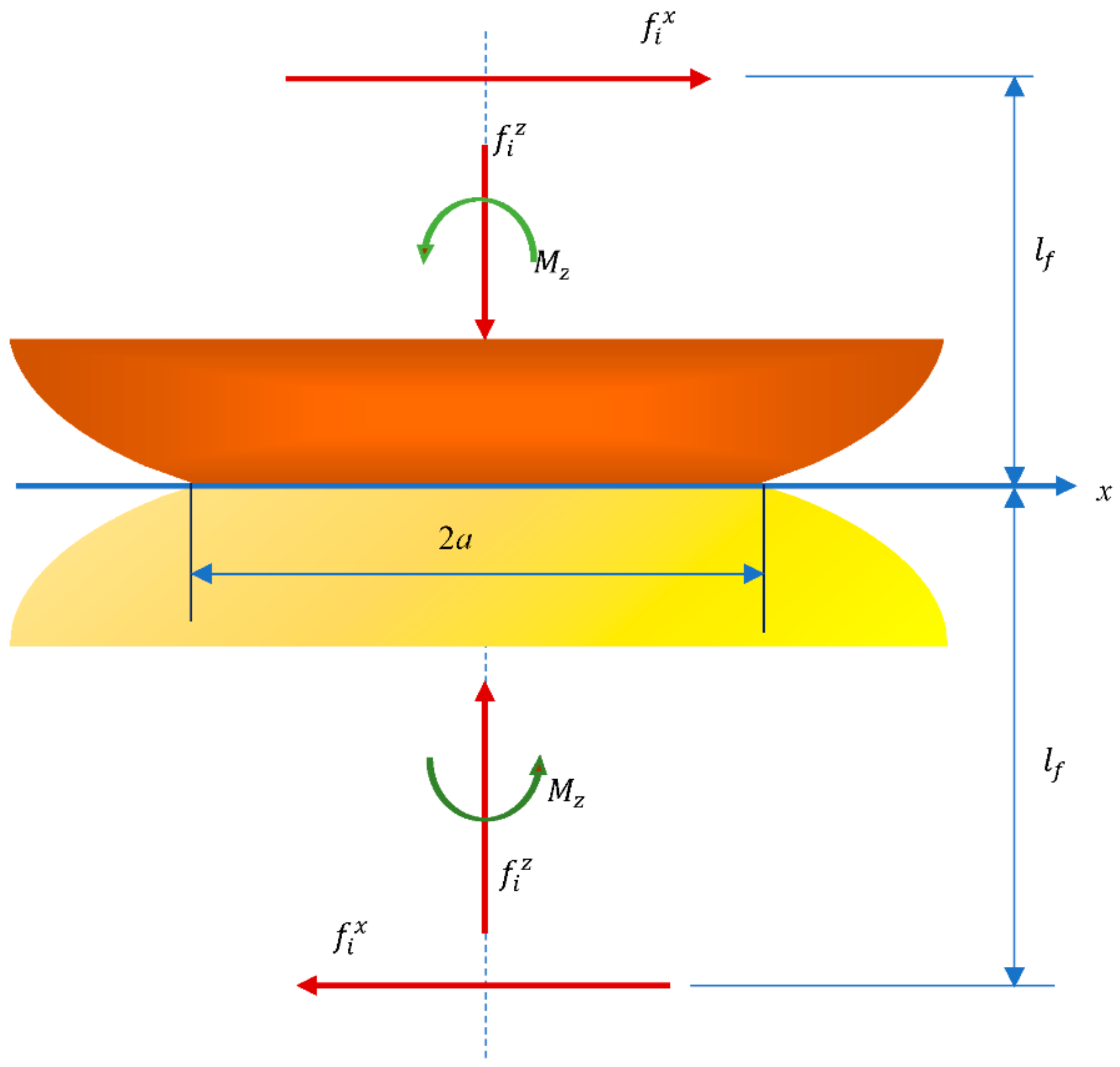
According to Mindlin [26], when two incompatible objects contact and squeeze, on the basis of the classical Hertz contact theory, the contact surface is considered as a circle. However, this consideration is only a special case for all the contact surface shapes so that it has no way to present the generalized contact shape, the conclusions derived from which can only be satisfied with quasi-static conditions because the friction is ignored. Therefore, during the derivation of the tangential stiffness, the normal stress is not the only parameter that should be taken into consideration, with the friction’s interaction not being neglected. According to this, the friction coefficient of every contact surface should be parameterized in this model, which could be defined as μi of the ith surface. To start the calculation, deriving the tangential stiffness along the direction of the x-axis becomes the first step so that only the force along the x-direction would be loaded besides the normal direction. Meanwhile, the elastic deformations along each axis Δx, Δy and Δz are considered as the function of the cartesian coordinates x, y and z. According to the geometric layout shown in Figure 1 and the Saint-Venant’s law, their geometric relationships could be presented as Equations (1)–(3):
where is a component of rigid-body displacement along the z-axis, the only one whose existence satisfies Saint-Venant’s law.

Figure 1.
The deformation between two contacting surfaces (along the x-axis).
To analyze its contact stiffness, those material parameters should be defined at the very beginning. We set the Poisson’s ratios of the i th contact surface-pair as and , so its mean ratio is
Further, we set their shear modules as and separately, which results in the mean shear modulus
We define a new operator as
According to the transition of force theory from Love [27], the elastic deformations , and at any point satisfy the potential function as
To make it convenient to calculate the deformation and stiffness, similar to the method of Johnson [2], we defined the potential functions , and as Equations (8)–(10):
where , and is the contact force between the i’s contact faces, is the area formed by the normal squeeze and is
and
where (, , ) are random points of the solid body and (, , ) are the general points of the . To make this calculation easier, let the surface , so .
Based on Love’s derivation of elastic deformation [27], the elastic deformation along the x, y and z-axis directions have the Equations (13)–(15):
and both and are satisfied with the Laplace equation so that
According to the classical Hertz contact theory, when the contact face is treated as a circle, the pressure on it is:
where is the contact radius and is the maximum pressure of the surface.
Analogically, the pressure on an elliptical contact surface could be carried out with a similar form as Equation (19)
With Equation (19), for any point at z = 0, to get its force component along the x-axis, when the direction is considered only along the x-axis, analogously, the force at z = 0 along the x-axis has the form of
where
To get the elastic deformation along the x-direction, Equation (20) has to be taken back to Equations (8) and (9) to make a simplification, then put the result back to Equations (13) and (14), eventually get two simplified equations as Equations (22) and (23):
where
Considering a prevalent situation where the contact slip progress is sustained over the whole contact surface, then it is noticed that φ could be replaced by φ-π in Equation (22), and every part containing φ of this equation could be substituted by 0, which could put an analogy in Equation (22) simultaneously. Therefore, Equations (22) and (23) could be simplified as Equations (29) and (30):
Thus far, the analysis is just for a slipping sphere. Considering the oscillating force theory of Johnson [2], this area is ring-shaped in geometry, with a radius range of . What is more, when analyzing the un-slipping sphere for the symmetrical characteristic, the loaded force component could be assumed as:
where
We put Equation (31) into the relative equations aforementioned to get another simplified result
Equation (29) can be added to Equation (33) to get a more simplified result; eventually, the elastic deformation along the x-axis could be derived as
To get the specific form of , the integration of the resultant force along the x-direction is needed, which is shown as Equation (36):
With Equation (36), could be solved as:
Take Equation (37) back to Equation (35), the elastic deformation along the x-axis could be solved as
Make a derivation of in Equation (38) to get the compliance along the x-axis
and the stiffness is the reciprocal of compliance, so the tangential stiffness along the x-axis, , is
Considering the rotation symmetry between the x and y-axis, likewise, the tangential stiffness along the y-axis , is
where is the major radius of the contact ellipse and is the minor one.
With the shape of the ellipse / and the ratio (/) of relative curvatures [2], the relationship between and could make an approximation as
Take into Equation (42), then
Based on the generalized Hertz theory of elastic contact [2], could be derived as
With Qin’s [28] result, could get an approximate result of
According to the result of Johnson [2] and Antonie [29], the equivalent radius of the contact face could be settled as:
where
Then, take Equation (46) back to Equation (45) to get the detailed expression of :
Put Equation (49) back to Equations (43) and (44), and bring the simplified result into Equations (40) and (41). Eventually, the tangential contact stiffness of i’s contact surfaces, and , is shown in Equations (50) and (51).
3. The Experiment Design for the Validation of the Modified Tangential Contact Stiffness Model
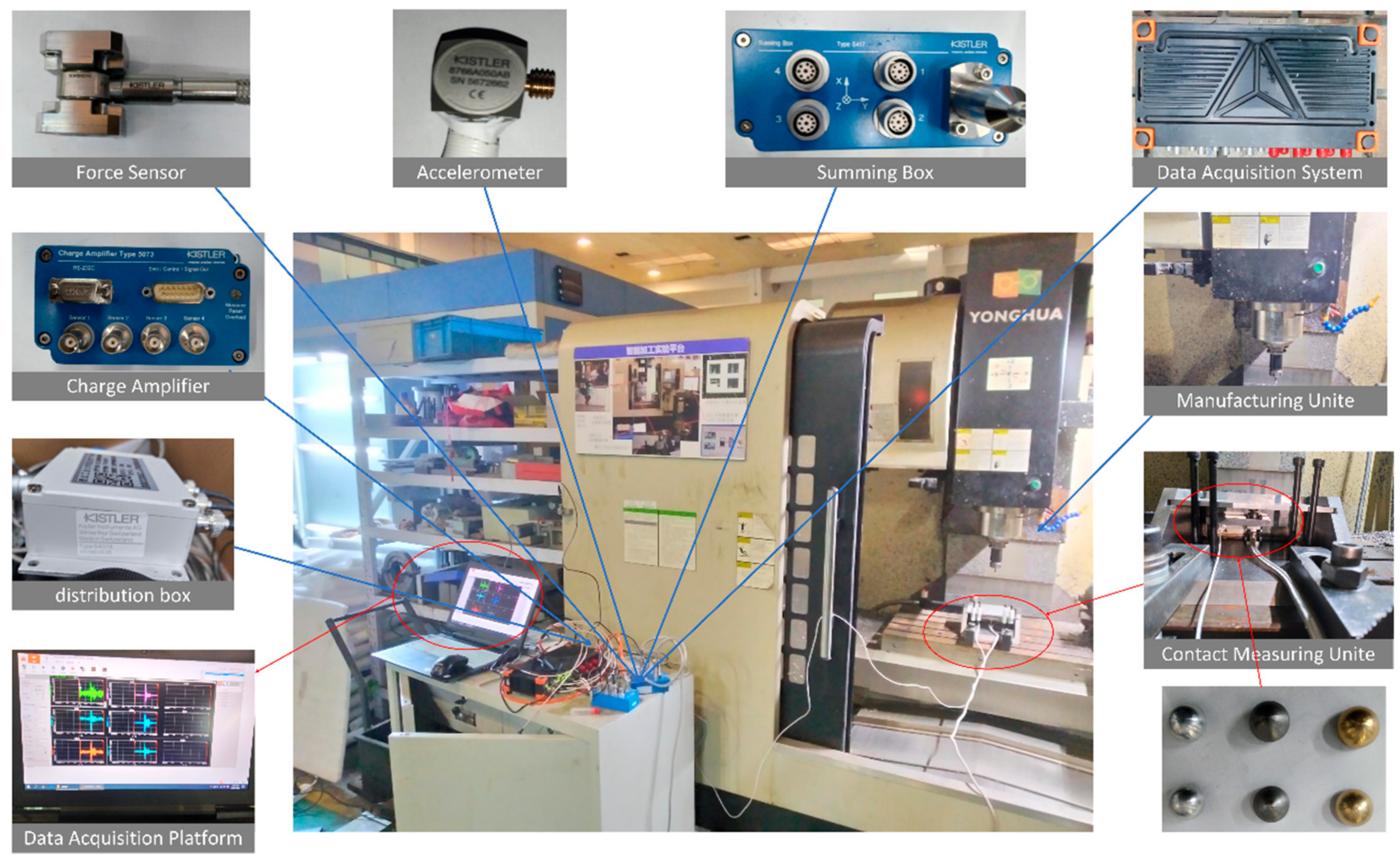
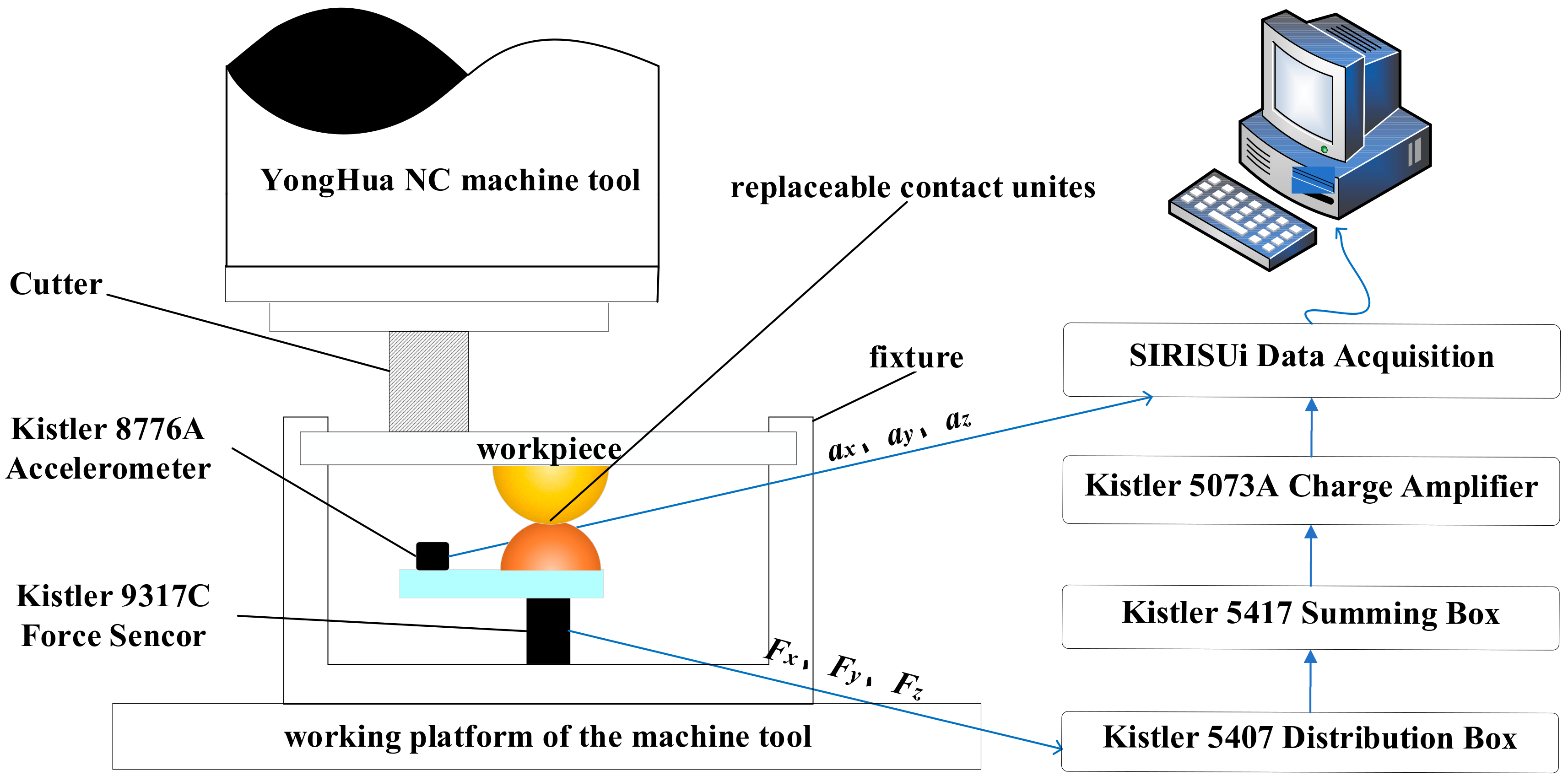
To validate the modified tangential contact stiffness model in this paper, an experiment to evaluate whether the model’s calculation is correct is necessary. Therefore, similar to Li [22], an experiment schedule to measure the tangential contact stiffness is provided, which turns out to be the key to verifying this model. For this purpose, a tangential-stiffness-measuring experiment platform is carried out, whose layout is presented in Figure 2, and its measurement result becomes the criterion of the accuracy of the model. The data collection and transmission process of this experiment are displayed in Figure 3.

Figure 2.
The experiment setup used in the tangential contact stiffness measuring.

Figure 3.
The data collection and transmission process of the modified tangential stiffness model validation experiment.
According to Equations (52) and (53), to get the tangential stiffness, the displacement of the contact area and and the contact force differences and of x and y-directions is necessary. and could be measured by the double integral acceleration signal of its relative direction, which could be collected by a Kistler 8776A triaxial IEPE accelerometer. The contact forces and could be gathered by a Kistler 9317C 3-component force link. Meanwhile, the frictional coefficient could be measured through the constant speed slide experiment with a spring dynamometer. The eventual goal is to calculate the relative error between the measured tangential contact stiffness and the predicted ones.
On closer inspection of Equations (50) and (51), it is clear that the contact radius and contact material are both parameters affecting the model’s eventual result. According to this, to assess their influence on the model, the design of the experiment with single parameter altering is necessary. However, this model belongs to statistics analysis, so there is no need to analyze its tendency during the manufacturing procedure. On this basis, the accuracy of this model is the only concern.
As discussed above, based on the eventual expression of this modified tangential contact model, the number of the influential parameters is so small that there is no need to design the experiment with a multifactor method. What is more, the attention should be paid to the purpose of this experiment, which is to validate the accuracy of this modified model in different ways, specifically speaking by means of altering every controllable parameter, and this is also the intention of Section 4 and Section 5, which is to analyze how these parameters would influence the model’s eventual accuracy.
For the controllable parameters, the contact radius and contact material, it is easy to know they are independent, obviously. Maybe some factors are left unanalyzed, e.g., the contact force and the frictional coefficient, but these factors are either dependent on existing factors or uncontrollable. Therefore, the contact radius and contact material are chosen as the factors to study, which also satisfies the intention of testing the modified model’s accuracy. The contact radius is essentially a length value, while the quantizable indicator of the material in this model is the mechanical characters E and G, which stand for the Yong’s modulus and shear modulus, respectively.
On these grounds, with the help of single-factor experiment design theory, a detailed experiment scheme is vividly portrayed. The number of the factors is fixed, and the change level of each parameter needs to be determined according to the experiment’s intention and the economic condition. As aforementioned, the validation of the model’s accuracy improvement is the main goal so that the total care of the scheme design is the economic condition and the parameter altering sequence. To get a relatively low economic cost, the materials tested in this experiment are Cu, Fe and Al. To fit the geometrical dimension of the sensors, the size of the radius is only set to 8 and 9 mm. It is possible the misgivings would come out that each parameter’s stage or level is too low, but in line with the experiment’s initial accuracy intention, this scheme design is enough. Based on the principle of a single-factor experiment design, the division of the experiment group should follow the rule that each group could change only one parameter from the previous neighboring one at a time. It is worth noting that for the pair number of the contact objects’ materials, there should be 3 × 3 = 9 groups to set up. However, three of them is just a change in the material contact order, such as Cu-Al to Al-Cu, so there is no need to repeat testing the same material pair again, and only six groups are indispensable. A similar scheme simplification method could be applied to the contact object’s radius, and that makes only two experiment groups left.
With this analysis, the detailed experiment scheme is listed in Table 1. In the table, R8 means the radius of the contact object is 8 mm, and R9 means 9 mm. √ means the parameter value related to the cell’s position are chosen in this table, and N/A means not chosen (not applicable).

Table 1.
The group deviation of the experiment schedule.
As shown in Table 1, the experiment schedule could be separated into two parts: the half evaluating material effectiveness and the half estimating radius function. The experiments considering the material parameters contain Groups 1 to 6, and the ones estimating the radius function include Groups 2, 5, 7 and 8.
The material’s effectiveness in this model mainly depends on its mechanical property, including Young’s modulus, shear modulus and Poisson ratio. To achieve this goal, three different materials, including Al, Fe and Cu, are selected, whose mechanical character data are listed in Table 2. The frictional coefficients among them measured with a spring dynamometer are listed in Table 3. By changing the material’s mechanical character in the model respectively, it would be possible to see whether the material’s characteristics could influence the model’s accuracy. The assessment of the radius’s role occurs in the same way.
Table 2.
The mechanical characteristics of selected materials.
Table 3.
The friction coefficient between selected materials.
4. Data Analysis of the Tangential Contact Stiffness Measuring and Model Validation
Along with the experiment schedule aforementioned, it is natural to divide the data analysis into two parts: the experiments with different contact materials and the ones with different contact radii. A noteworthy fact is that the model verified is a static one, so there is no need to put data along the whole process of every experiment for the analysis. Meanwhile, each data group contains more than 10,000 arrays, and if all these data are thickly dotted in one figure, it will be impossible to find the pattern and assess its accuracy. Above all, to make the result clearer and the figure more visible, every experiment’s result will have 30 arrays chosen randomly, which results in the best visualization because of the suitable data density in the figure, as the foundation of the data analysis below.
4.1. Experiments with Different Contact Materials
These experiments mainly include but are not restricted to, Groups 1–6.
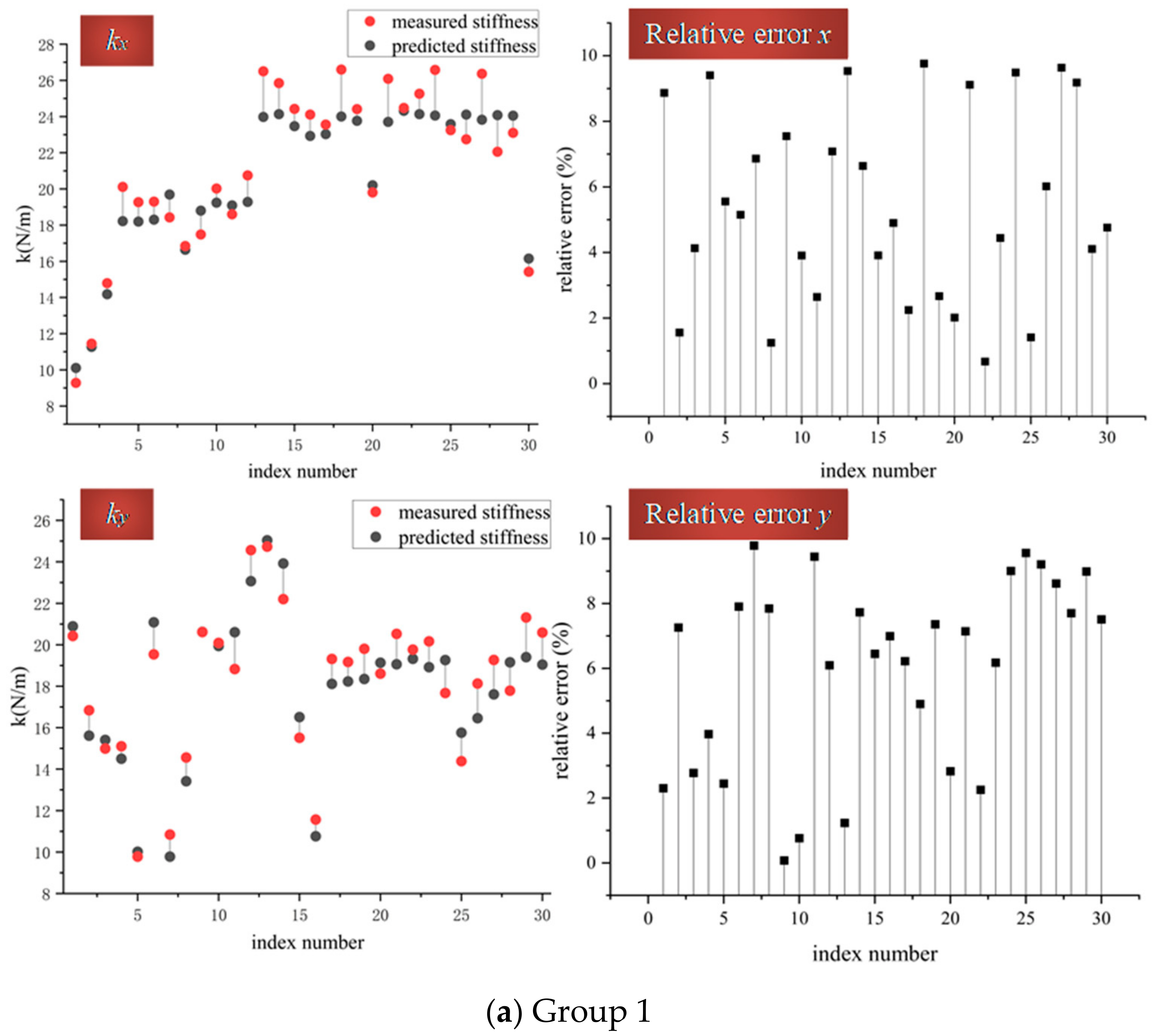
In Figure 4, and in the following sections, kx means the tangential contact stiffness of the x-axis, and ky represents the tangential contact stiffness of the y-axis. For both of these two measurements, the relative error is:
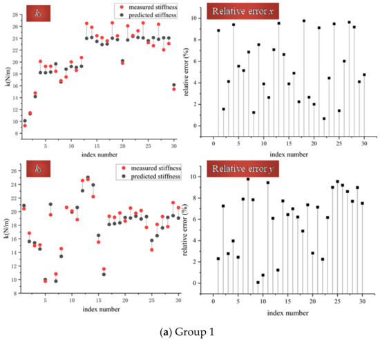
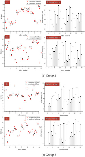
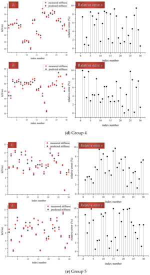
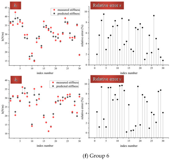
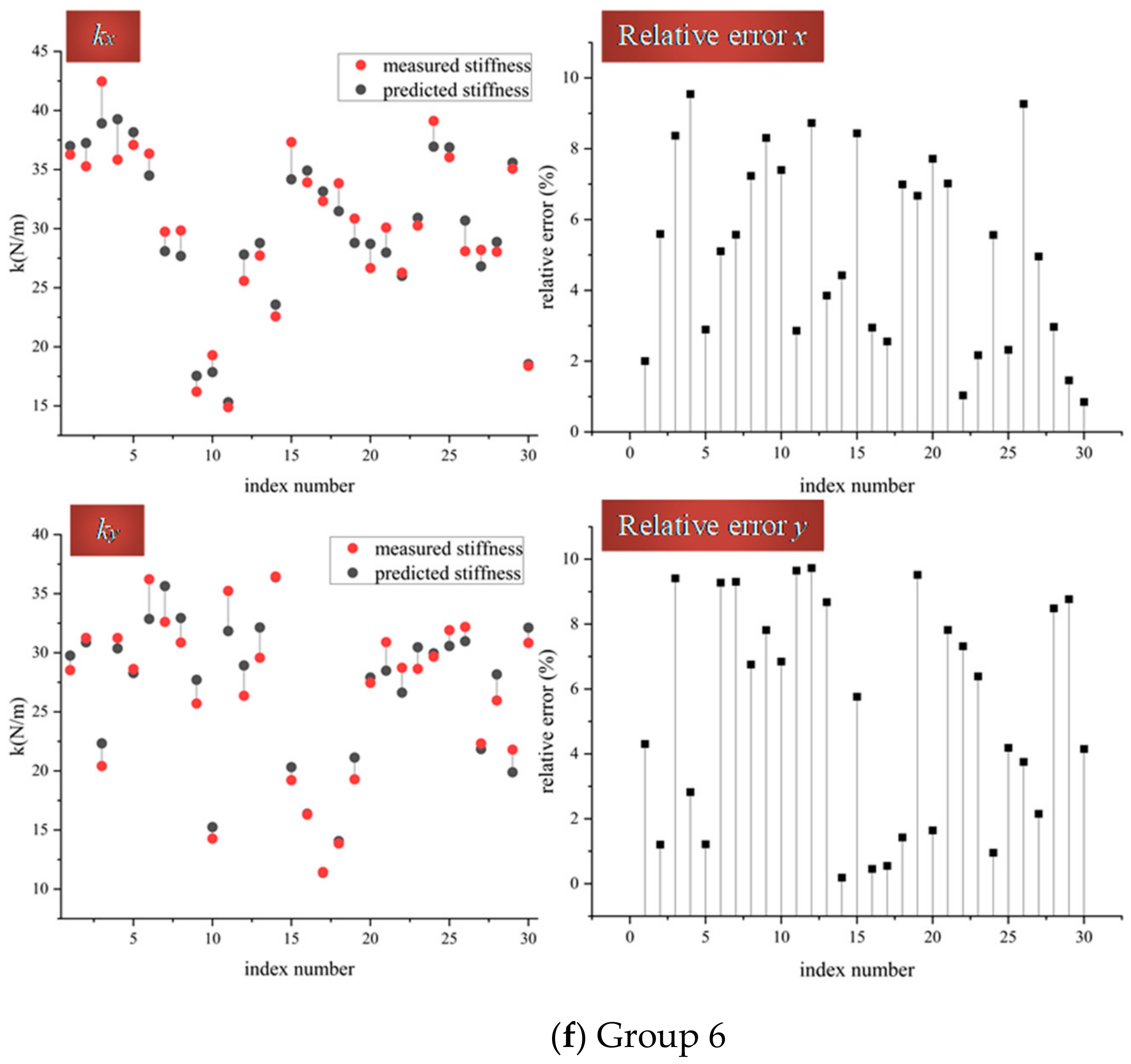
Figure 4.
The comparison of tangential contact stiffness between measured ones and predicted ones among different materials.
In general, the relative error between the measured tangential stiffness and the predicted one is less than 10%. More specifically, to estimate the material mechanical parameter’s role in the model’s accuracy, six experimental groups, including three different materials, have been arranged. Logically, there should be 3 × 3 = 9 groups to be set up. However, three of them are just changes in the material contact order, such as Cu-Al to Al-Cu, so there is no need to repeat testing the same material pair again, and only six groups are indispensable.
In Group 1, the material of the contact pair is Cu and Cu, with radii of 8 and 9 mm. Relatively, Group 2 only changes half of this pair to another material, Fe, with the other parameters fixed. Comparing the results of these two groups, it is implicit to find out the difference. Because of the random data chosen, the results displayed do not stand for any tendency meaning, which is not the focus of the experiment.
On the other hand, it could be concluded that the change of material has almost no influence on the model’s accuracy. In Group 1, the largest relative error is 9.7%, while in Group 2, the largest relative error is 9.9%, which is almost the same as Group 1. This conclusion is also appliable to the rest of the experimental groups: from Group 2 to Group 3, the only changed parameter is the material from Fe to Al, but the largest relative error is 9.8%; from Group 2 to Group 4, the only changed parameter is the material from Cu to Fe, and the largest relative error is 10%; from Group 4 to Group 5, the only changed parameter is the material from Fe to Al, and the largest relative error is 9.9%; from Group 5 to Group 6, the only changed parameter is the material from Fe to Al, and the largest relative error is 9.9%. Above all, as our experiment schedule is constructed, in every group of experiments, only one parameter alters compared to its proximate one. While according to the data aforementioned, there is barely any difference in the accuracy of these groups, and this could verify the conclusion that the change of material has almost no influence on the model’s accuracy.
4.2. Experiments with Different Radius
Although these experiments’ designs depend on the principle of single-parameter control, the comparing experiments mainly include but are not restricted to, Groups 7 and 8.
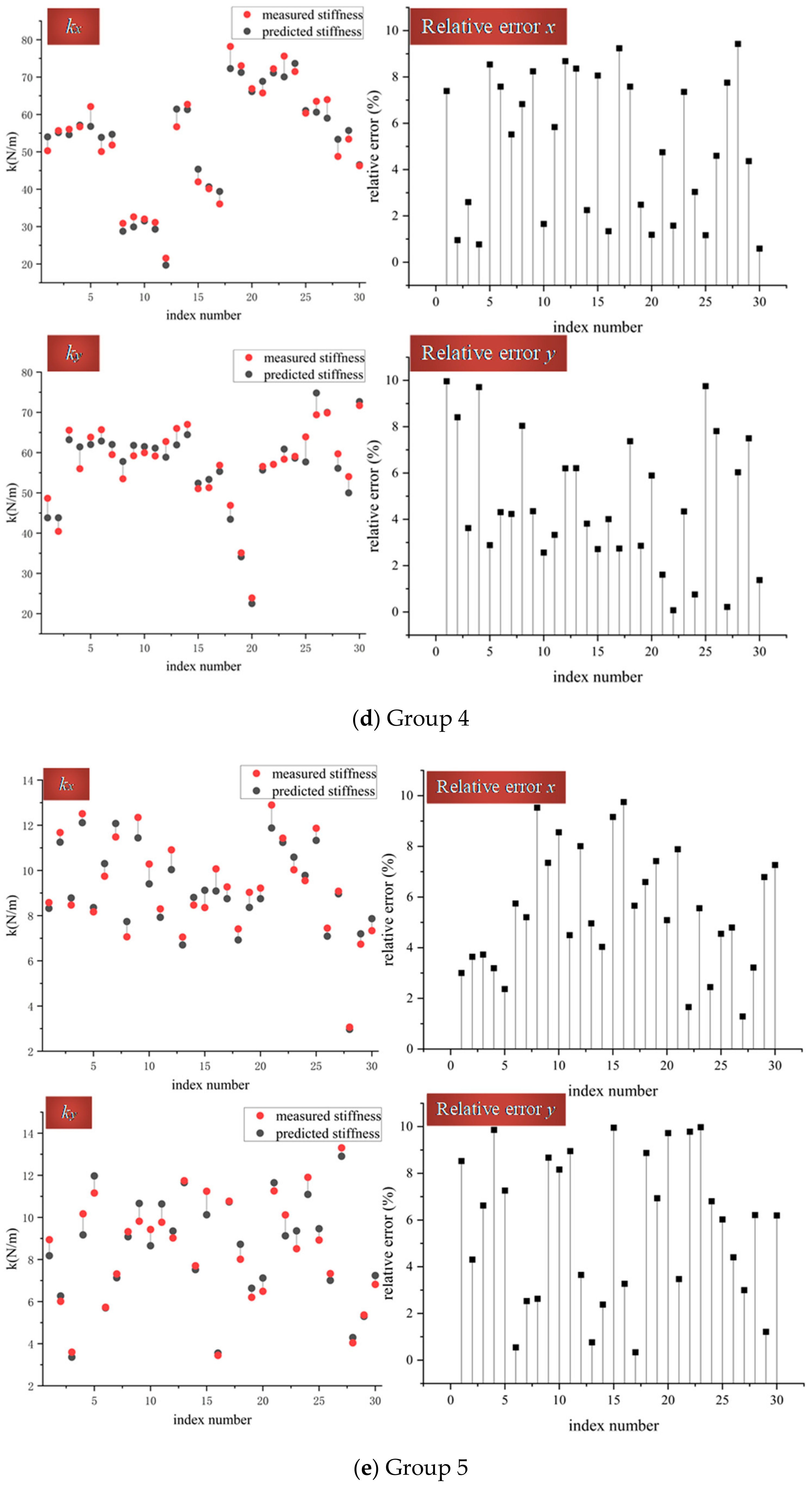
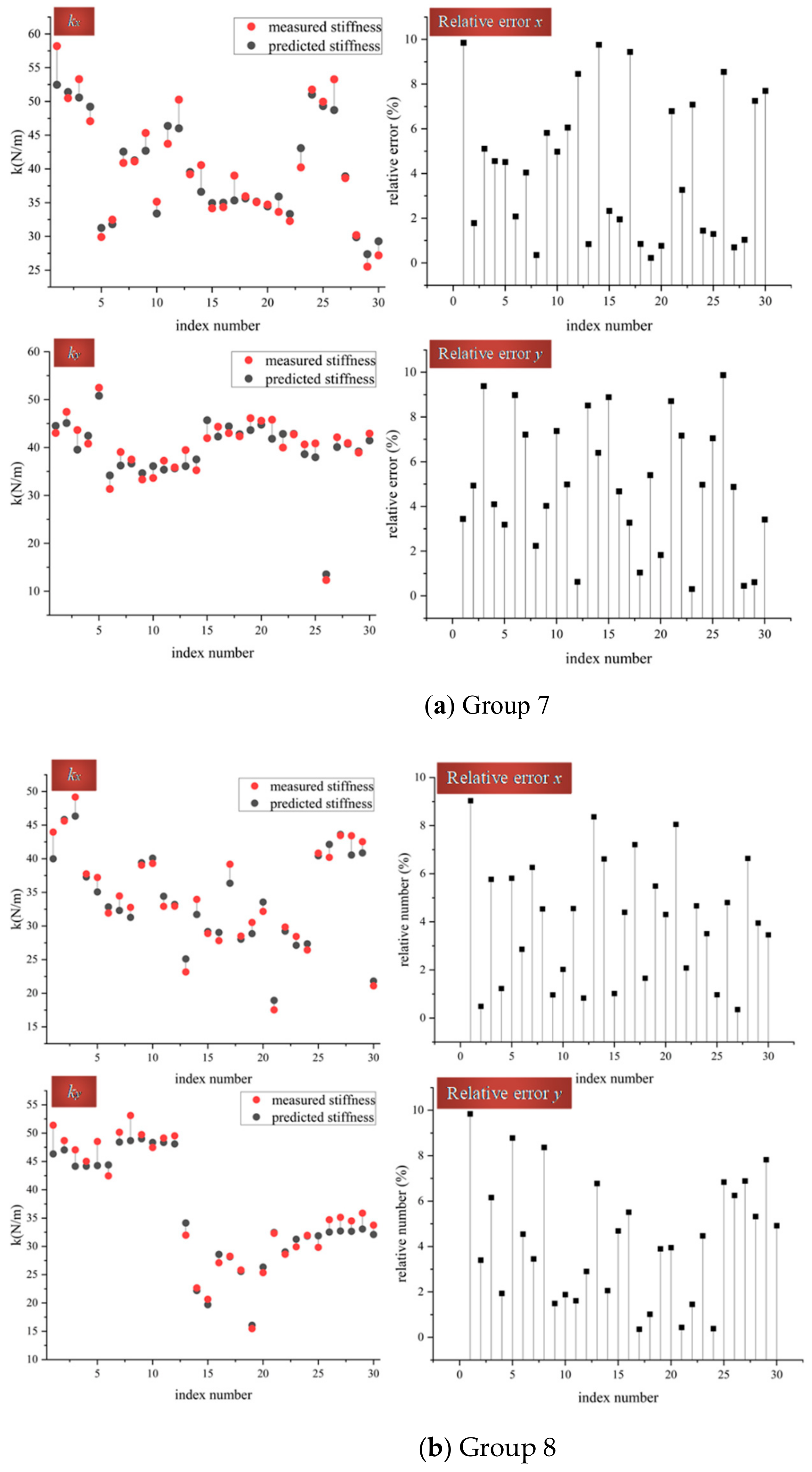
In Figure 5, the meaning of the symbols is the same as in Figure 4, and, in general, similar to the phenomena above, the relative error between the measured tangential stiffness and the predicted one is less than 10%. More specifically, to estimate the contact object radius’s role in the model’s accuracy, two experimental groups, including two different radii (8 and 9 mm), have been arranged, accompanying the relevant groups: Groups 2 and 5.
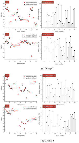
Figure 5.
The comparison of tangential contact stiffness between measured ones and predicted ones among different radii.
In Group 7, the materials of the contact pair are Cu and Fe, with the radii of 8 mm and 8mm. Compared with Group 2, only one radius of half of the contact pair has been changed, while the other parameters are fixed. Putting together these two groups’ experiment results, there are inconspicuous differences between them, which is the same phenomenon of experiments with different contact materials above.
The analogic conclusion is that the change of the radius has almost no influence on the model’s accuracy. In Group 7, the largest relative error is 9.9%, while in Group 2, the largest relative error is 9.9% which is almost the same as Group 7. The comparison between Group 8 and Group 5 has the analogous situation to Group 7 and Group 2: in Group 8, the largest relative error is 9.8%, while in Group 3, the largest relative error is 9.9%, which is almost the same as Group 8. However, the only difference between Group 8 and Group 3 is the radius, which verifies that the change of the contact object’s radius plays an infinitesimal role of the tangential contact stiffness model’s accuracy.
5. Comparison between the Model with and without Friction’s Effect
Before an elaborate analysis of the model’s improvement, a comparison or a filtration process of the models similar to the modified model is inevitable, which is to shorten the comparison process and pay more attention to the comparison with the research closest to this paper. After a wide search, there are three models in recent mainstream researches that are similar to our model, which are listed in Table 4.
Table 4.
The comparison between similar mainstream tangential contact stiffness models.
To clarify the statement, the tangential contact stiffness model deduced in this paper could be named the Modified Model. Comparing the Modified Model with Model 2 [30], it is convenient to find that Model 2 has lost an item , which is a significant factor of the slip effect caused by the friction, professionally speaking, an elliptical contact sphere, but universally, a general contact form. This neglect in Model 2 has lost the effect of slip, which would cause a great gap from the true value. Focusing on Model 3 [31], a simpler model compared to Model 2, the variable in it only has . This simplification only holds the influence of the normal contact force, while the influence of the contact shape and the tangential friction is disregarded. This tremendous simplification is only suitable for some iteration steps where the high calculation speed is initial, but its accuracy is so poor that its application range is too narrow. The only model left is Model 1 [28], which is the most similar model of recent studies to the Modified Model in this paper. The difference, or the improvement, of our work is presented elaborately below.
To clarify the statement, the model deduced by Qin [28] (Model 1) can be called the original model. From Table 5, it is obvious to see that the difference between the original model and the modified one is mainly focused on the radius of each contact sphere and the contact force of the contact area along the direction of the x, y and z-axis. The modified model has taken the contact force into consideration, mainly because of the reduction as little as possible during the model’s deduction. In the original model, the particular character terms are and , which are constant parameters when materials and the shapes of both contact objects fixed. Compared to this, the modified model has some additional terms and , and this could be treated as a function of the contact force, which means it is a variable parameter.
Table 5.
The comparison between the original model and the modified model.
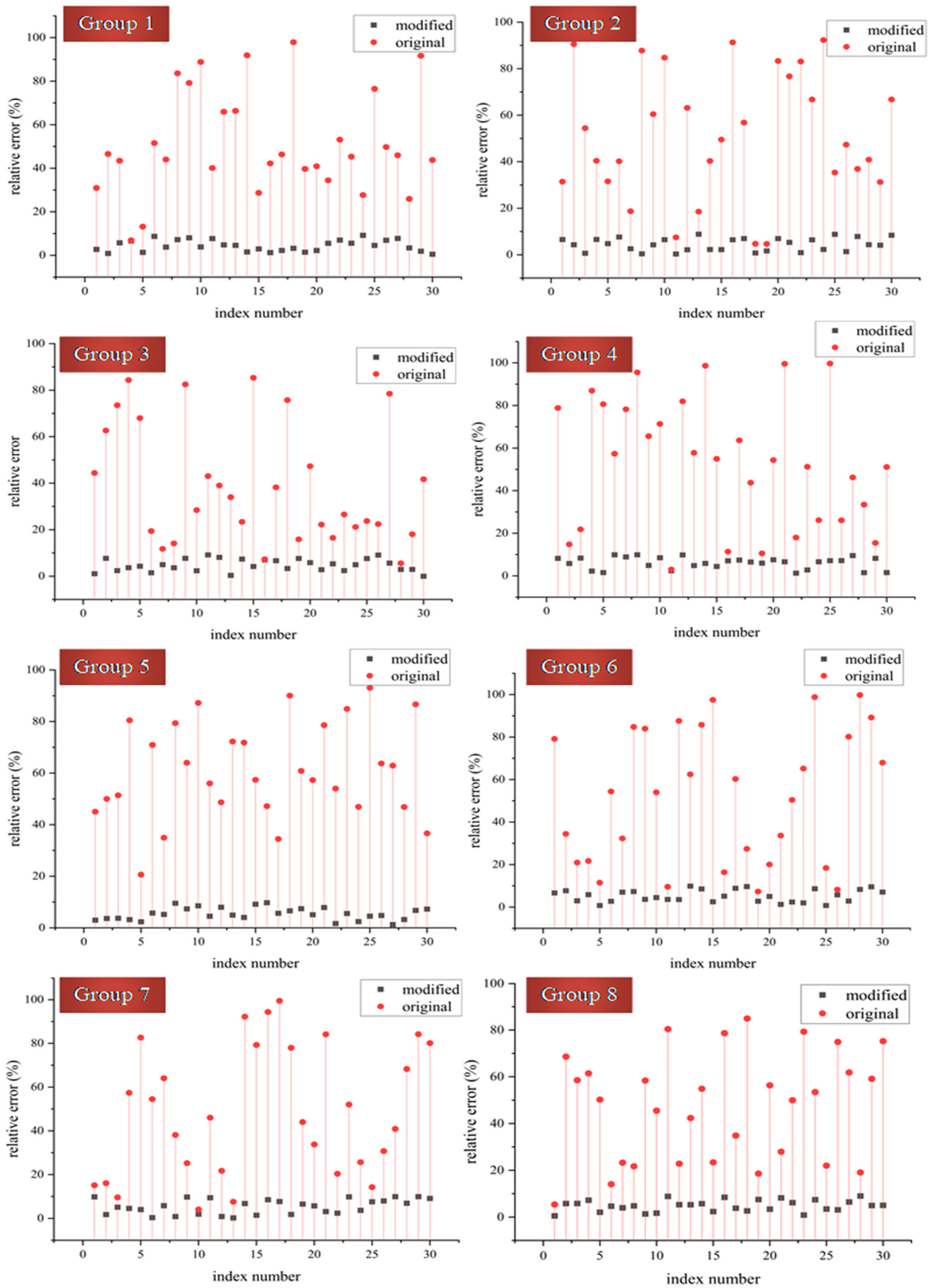
In order to figure out how much influence this change has on the accuracy of the modified model, the calculation based on experimental data for both models is inevitable. The experimental data collected in Section 4 could be employed to continue this work. The relative errors of both the original model and the modified one are calculated as the evaluating indicator of this process, classified into two groups: the ones along the x-direction and those along the y-direction. The results are shown in Figure 6 and Figure 7.
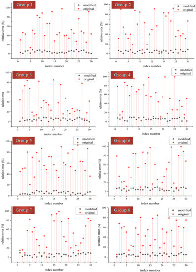
Figure 6.
The comparison of model accuracy based on the data along the x-axis.
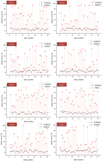
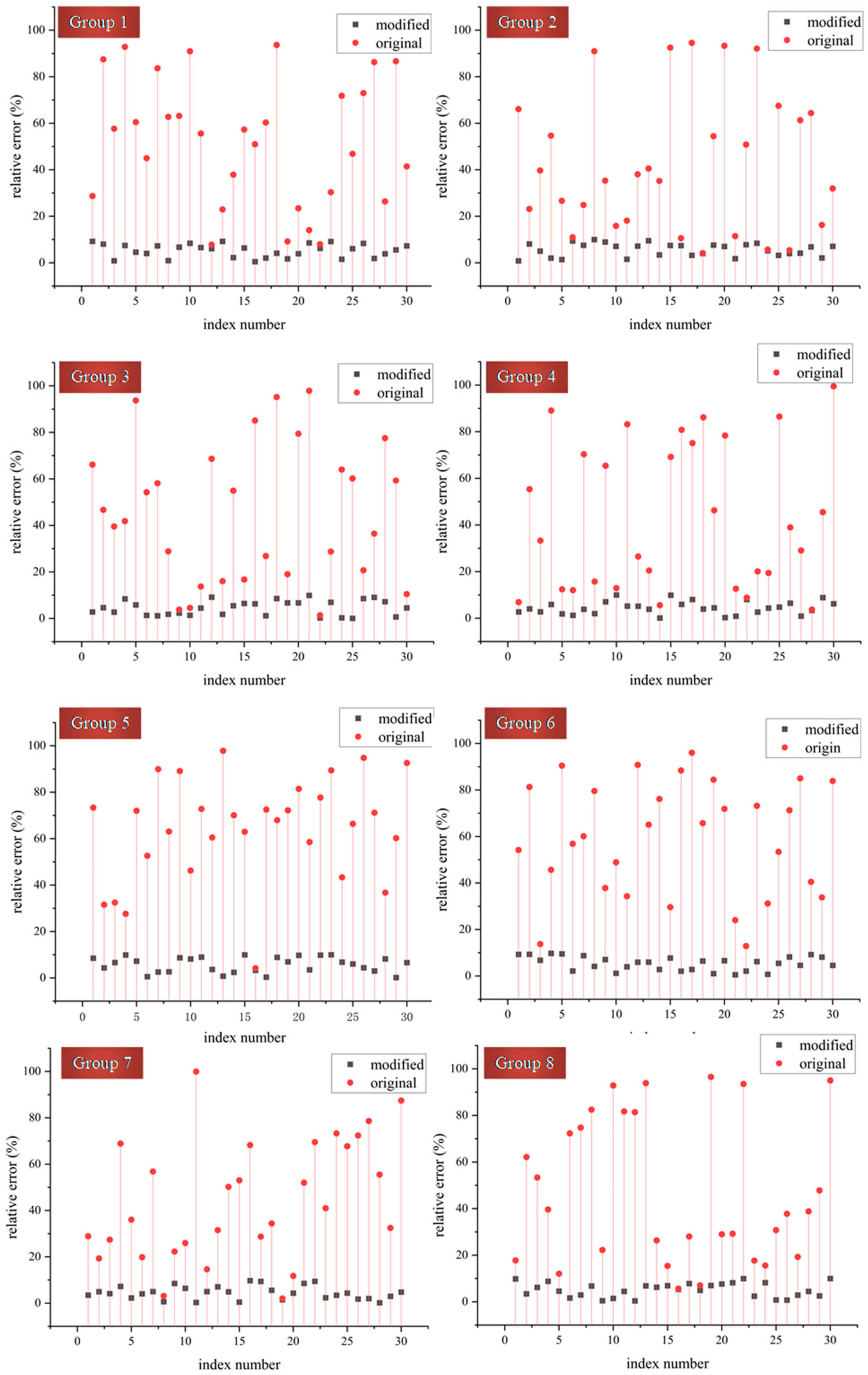
Figure 7.
The comparison of model accuracy based on the experienced data along the y-axis.
5.1. Model Accuracy Comparison along the x-Axis
To make the comparison result visible for analysis, it is necessary to narrow the data scale presented in one picture. Picking out 30 sets of data from each group randomly seems to be an excellent choice for this data visualization process. As is depicted in Figure 6, the relative error of the original model is apparently bigger than the modified one, which is the key point to present the improvement to the research from this paper. Specifically, in the original model, the relative error above 50% occupies more than half of the 30 data sets in each of these 8 groups, and only one-quarter of these groups’ relative errors are below 30% in half of the data sets. Compared with the modified model, the difference is too overt to see. The relative errors of the modified model in these eight groups are all below 10%, and that means the variance of the modified model’s relative error is much smaller than the original one. What is more, in Groups 1, 2 and 4, the relative error of the modified model is much smaller than the original one for most of the data sets of each group.
5.2. Model Accuracy Comparison along the y-Axis
Each group has been taken 30 sets of data randomly. As shown in Figure 7, the similar phenomenon from the x-direction could be carried out so that the relative error of the modified model is much smaller than the original one. Specifically, in the original model, a relative error above 50% occupies more than 3/4 of the 30 data sets in each of these 8 groups, and only 1/4 of these groups’ relative error is below 30% in half of the data sets, such as Groups 4 and 7. While comparing with the relative errors of the modified model in these 8 groups, they are all less than 10%, which is similar to the relative error of the tangential stiffness model along the x-axis. What is more, in Groups 5, 6 and 8, the relative error of the modified model is much smaller than the original one for most of the data sets of each group.
6. The Discrepancy Analysis between the Model Calculation and the Experiment Measurement
To make it clear whether the discrepancy between the modified model’s prediction result and the experiment’s measurement is larger or the margin of the measure equipment’s error is bigger, it is inevitable to analyze the error from this measuring progress. The experiment platform’s elements are presented in Figure 2, and to get the whole platform’s instrument error, every element’s error band is necessary, as listed in Table 6.
Table 6.
The error band of each element in the modified experiment’s platform.
According to Equations (52) and (53), the tangential stiffness along the x and y-axis’s measurement is the deformation divided by the force increment of their direction, respectively, which means the error propagation analysis of A/B is inevitable. With the symmetry character of the tangential stiffness model along the x and y-axis, only the stiffness along the x-axis is discussed in this section. According to Ammar Grous [32], the error of the tangential stiffness along the x-axis can be expressed as Equation (55):
According to this expression and Table 6, it is not hard to get the foundation of this error band: , , and . To get the range of , the range of each parameter in is essential, which means the maximum and minimum value of each parameter is necessary. Based on Table 6, it is convenient to see that is larger than by at least 16 orders of magnitude; therefore, Equation (55) can be simplified as:
where is the infinitely small term of and then the simplification of Equation (56) could be justified. The data listed in Table 6 manifests that is at least one magnitude smaller than the discrepancy between the model value and the experimental data. According to the symmetry character of the tangential stiffness model along the x and y-axis, the error of the tangential stiffness along the y-axis will have a same magnitude character as . And that means the change from the modified model is not from the discrepancy between the experiment and the model’s calculation but an effective improvement of the original one.
7. Conclusions
This paper focuses on the study of the mechanical structure contact mechanism considering modified tangential stiffness with friction’s interaction. A tangential contact stiffness model considering friction’s interaction is constructed. The derivation process of this model begins with Love’s elastic deformation theory along the x, y and z-axis, whose construction contains the potential function along with their own direction respectively. The generalized Hertz contact theory is used to calculate the forces needed in this model. With the help of the symmetrical characteristics in the contact area, the derivation process is simplified, and the tangential contact stiffness model considering independent variables, which are the contact force along the x, y and z-axis and the friction coefficient of the contact area, is eventually carried out; these variables are barely considered simultaneously in the model construction of the tangential contact stiffness in previous research.
To verify this model, a tangential stiffness measuring platform is constructed by putting two spherical objects into contact with each other to measure the tangential contact stiffness. The relative displacement and the contact force of the contact area are calculated with the data collected by a force sensor and accelerometer connected to the PC Dewesoft client. With a deeper analysis of the effect of the model’s parameter, an experimental scheme based on single-parameter control (material mechanical character and contact radius) containing eight groups is carried out. The relative errors of the tangential contact stiffness model are all less than 10% for each data group in the experiment.
A comparison with an existing model is carried out. The evaluation indicator of the comparison is the relative error of the tangential stiffness, along with the directions of the x and y-axis, respectively. The results show that the model deduced in this research has a much better performance than the original one. Along the direction of the x-axis, the relative error of the original model over 50% occupies more than half of the 30 data sets in each of these 8 groups, and only 1/4 of these groups’ relative error is below 30% in half of the data sets; along the direction of the y-axis, the original model’s relative error exceeded 50% captures in more than 3/4 of the 30 data sets in each of these 8 groups, and only 1/4 of these groups’ relative error below 30% in half of the data sets. While the relative errors of the modified model are all less than 10% on the foundation of the same data sets. This could show the advantage of the modified contact tangential model proposed in this paper. In summary, the correctness of the modified tangential contact stiffness model is verified by the experiment, and that means the mechanical structure contact mechanism analysis considering modified tangential stiffness with friction’s effect is effective. This improved tangential contact stiffness model, the first key step in establishing a systematic dynamic model, would be an effective improvement for the fixture-workpiece system dynamic analysis, which is eventually an inevitable foundation of vibration reduction for aerospace blade manufacturing.
Author Contributions
Z.N.: first author, constructed the model, interpreted the data, drafting, performed the numerical calculation and milled the experiments. B.C.: corresponding author, proposed the starting model modified idea, checked the proposed method, edited the manuscript and provided the funding. H.C.: improved the figures of this manuscript and modified the model’s derivation. J.H.: optimized the experiment’s design and carred out the experiment schedule. J.Q.: edited the manuscript and discused the model’s application prospect. M.W.: edited the manuscript and provided the funding. All authors have read and agreed to the published version of the manuscript.
Funding
This work was supported by the National Key R&D Program of China (No. 2019YFB1703802). Thanks are also given to the Natural Science Foundation of Shaanxi (Grant No. 2022JM-192).
Institutional Review Board Statement
This article does not contain any studies with human participants or animals performed by any of the authors.
Informed Consent Statement
Not applicable.
Data Availability Statement
The datasets generated during and/or analyzed during the current study are available from the corresponding author on reasonable request.
Conflicts of Interest
The authors declare no conflict of interest.
References
- Stronge, W.J. Impact Mechanics, 2nd ed.; Cambridge University Press: Cambridge, UK, 2018; ISBN 978-0-521-84188-7. [Google Scholar]
- Johnson, K.L. Contact Mechanics, 1st ed.; Cambridge University Press: Cambridge, UK, 1987; ISBN 0521255767. [Google Scholar]
- Yang, H.P.; Che, X.W.; Yang, C. Investigation of normal and tangential contact stiffness considering surface asperity interaction. Ind. Lubr. Tribol. 2020, 3, 379–388. [Google Scholar] [CrossRef]
- Medina, S.; Nowell, D.; Dini, D. Analytical and numerical models for tangential stiffness of rough elastic contacts. Tribol. Lett. 2013, 49, 103–115. [Google Scholar] [CrossRef]
- Pan, W.; Li, X.; Wang, L.; Guo, N.; Mu, J. A normal contact stiffness fractal prediction model of dry-friction rough surface and experimental verification. J. Theor. Appl. Mech. 2017, 66, 94–102. [Google Scholar] [CrossRef]
- Sherif, H.A. Mode of zero wear in mechanical systems with dry contact. Tribol. Int. 2004, 38, 59–68. [Google Scholar] [CrossRef]
- Parel, K.S.; Paynter, R.J.; Nowell, D. Linear relationship of normal and tangential contact stiffness with load. Proc. R. Soc. A 2020, 476, 20200329. [Google Scholar] [CrossRef]
- Pierre, J.; Pierre, L.; Adnan, I. Initial versus tangent stiffness-based Rayleigh damping in inelastic time history seismic analyses. Earthq. Eng. Struct. Dyn. 2014, 43, 467–484. [Google Scholar] [CrossRef] [Green Version]
- Sultan, C. Stiffness formulations and necessary and sufficient conditions for exponential stability of prestressable structures. Int. J. Solids Struct. 2013, 50, 2180–2195. [Google Scholar] [CrossRef] [Green Version]
- Mobasher, B.; Peled, A.; Pahilajani, J. Distributed cracking and stiffness degradation in fabric-cement composites. Mater. Struct. 2006, 39, 317–331. [Google Scholar] [CrossRef]
- Woodward, P.; Kennedy, J.; Laghrouche, O.; Connolly, D.P.; Medero, G. Study of railway track stiffness modification by polyurethane reinforcement of the ballast. Transp. Geotech. 2014, 1, 214–224. [Google Scholar] [CrossRef]
- Bernal, D. Instability of buildings during seismic response. Eng. Struct. 1998, 20, 496–502. [Google Scholar] [CrossRef]
- Romanoff, J.; Remes, H.; Socha, G.; Jutila, M.; Varsta, P. The stiffness of laser stake welded T-joints in web-core sandwich structures. Thin Walled Struct. 2007, 45, 453–462. [Google Scholar] [CrossRef]
- Zhao, Y.; Han, Z.; Ma, Y.; Zhang, Q. Establishment and verification of a contact model of flowing fresh concrete. Eng. Comput. 2017, 35, 2589–2611. [Google Scholar] [CrossRef]
- Fukagai, S.; Marshall, M.B.; Lewis, R. Transition of the friction behaviour and contact stiffness due to repeated high-pressure contact and slip. Tribol. Int. 2022, 170, 107487. [Google Scholar] [CrossRef]
- Kakogawa, A.; Kawabata, T.; Ma, S. Plate-springed parallel elastic actuator for efficient snake robot movement. IEEE ASME Trans. Mechatron. 2021, 26, 3051–3063. [Google Scholar] [CrossRef]
- Stabile, C.J.; Levine, D.J.; Iyer, G.M.; Majidi, C.; Turner, K.T. The role of stiffness in versatile robotic grasping. IEEE Robot. Autom. Lett. 2022, 7, 4733–4740. [Google Scholar] [CrossRef]
- Zaare, S.; Soltanpour, M.R. Adaptive fuzzy global coupled nonsingular fast terminal sliding mode control of n-rigid-link elastic-joint robot manipulators in presence of uncertainties. Mech. Syst. Signal Process. 2022, 163, 108165. [Google Scholar] [CrossRef]
- Zhang, X.; Wang, N.; Lan, G.; Wen, S.; Chen, Y. Tangential damping and its dissipation factor models of joint interfaces based on fractal theory with simulations. J. Tribol. 2014, 136, 011704. [Google Scholar] [CrossRef]
- Shi, J.; Cao, X.; Zhu, H. Tangential contact stiffness of rough cylindrical faying surfaces based on the fractal theory. J. Tribol. 2014, 136, 041401. [Google Scholar] [CrossRef]
- Eriten, M.; Chen, S.; Usta, A.D.; Yerrapragada, K. In situ investigation of load-dependent nonlinearities in tangential stiffness and damping of spherical contacts. J. Tribol. 2021, 143, 061501. [Google Scholar] [CrossRef]
- Li, D.; Botto, D.; Xu, C.; Liu, T.; Gola, M. A micro-slip friction modeling approach and its application in underplatform damper kinematics. Int. J. Mech. Sci. 2019, 161–162, 105029. [Google Scholar] [CrossRef]
- Zheng, Y.; Rong, Y.; Hou, Z. The study of fixture stiffness part I: A finite element analysis for stiffness of fixture units. Int. J. Adv. Manuf. Technol. 2008, 36, 865–876. [Google Scholar] [CrossRef]
- Zheng, Y.; Hou, Z.; Rong, Y. The study of fixture stiffness—Part II: Contact stiffness identification between fixture components. Int. J. Adv. Manuf. Technol. 2008, 38, 19–31. [Google Scholar] [CrossRef]
- Balaji, N.N.; Dreher, T.; Krack, M.; Brake, M.R. Reduced order modeling for the dynamics of jointed structures through hyper-reduced interface representation. Mech. Syst. Signal Process. 2021, 149, 107249. [Google Scholar] [CrossRef]
- Mindlin, R.D.; Mason, W.P.; Osmer, T.F.; Deresiewicz, H. Effects of an oscillating tangential force on the contact surfaces of elastic spheres. In Proceedings of the First US National Congress of Applied Mechanics, Chicago, IL, USA, 11–16 June 1951; pp. 203–208. [Google Scholar]
- Love, A.E.H. A Treatise on the Mathematical Theory of Elasticity, 4th ed.; Cambridge University Press: Cambridge, UK, 2013; ISBN 9781107618091. [Google Scholar]
- Qin, G.; Zhang, W.; Wan, M. A machining-dimension-based approach to locating scheme design. J. Manuf. Sci. Eng. 2008, 130, 051010. [Google Scholar] [CrossRef]
- Antoine, J.-F.; Visa, C.; Sauvey, C.; Abba, G. Approximate analytical model for hertzian elliptical contact problems. J. Tribol. 2006, 128, 660–664. [Google Scholar] [CrossRef]
- Guan, D.; Jing, L.; Hilton, H.H.; Gong, J.; Yang, Z. Tangential contact analysis of spherical pump based on fractal theory. Tribol. Int. 2018, 119, 531–538. [Google Scholar] [CrossRef]
- Dong, H.; Qiu, C.; Prasad, D.K.; Pan, Y.; Dai, J.; Chen, I.-M. Enabling grasp action: Generalized quality evaluation of grasp stability via contact stiffness from contact mechanics insight. Mech. Mach. Theory 2019, 134, 625–644. [Google Scholar] [CrossRef]
- Ammar, G. Applied Metrology for Manufacturing Engineering; John Wiley & Sons: Hoboken, NJ, USA, 2011; ISSN 978-1-84821-188-9. [Google Scholar]

Publisher’s Note: MDPI stays neutral with regard to jurisdictional claims in published maps and institutional affiliations. |
© 2022 by the authors. Licensee MDPI, Basel, Switzerland. This article is an open access article distributed under the terms and conditions of the Creative Commons Attribution (CC BY) license (https://creativecommons.org/licenses/by/4.0/).