Article

MatNERApor—A Matlab Package for Numerical Modeling of Nonlinear Response of Porous Saturated Soil Deposits to P- and SH-Waves Propagation

by
Artem A. Krylov
1,2,3,*,
Sergey A. Kovachev
1,
Elena A. Radiuk
1,
Konstantin A. Roginskiy
1,
Mikhail A. Novikov
1,4,
Olga S. Samylina
5,
Leopold I. Lobkovsky
1,2,4 and
Igor P. Semiletov
2,3
1
Shirshov Institute of Oceanology, Russian Academy of Sciences, 36, Nakhimovskiy Prospekt, 117997 Moscow, Russia
2
V.I. Il’ichev Pacific Oceanological Institute, Far Eastern Branch of the Russian Academy of Sciences, 43, Baltijskaya St., 690041 Vladivostok, Russia
3
Institute of Ecology, National Research University Higher School of Economics (HSE), 11, Pokrovskiy Bulvar, 109028 Moscow, Russia
4
Moscow Institute of Physics and Technology, 9, Institutsky Lane, 141700 Dolgoprudny, Russia
5
Winogradsky Institute of Microbiology, Research Center of Biotechnology, Russian Academy of Sciences, 7/2, Prospect 60-Letiya Oktyabrya, 117312 Moscow, Russia
*
Author to whom correspondence should be addressed.
Appl. Sci. 2022, 12(9), 4614; https://doi.org/10.3390/app12094614
Submission received: 2 April 2022 / Revised: 29 April 2022 / Accepted: 1 May 2022 / Published: 4 May 2022
(This article belongs to the Special Issue State-of-Art of Soil Dynamics and Geotechnical Engineering)

Abstract

:
The paper is devoted to the problem of numerical modeling of earthquake response of porous saturated soil deposits to seismic waves propagation. Site-specific earthquake response analysis is a necessary and important component of seismic hazard assessment. Accounting for the complex structure of porous saturated soils, i.e., the content in them, in addition to the solid matrix, pore water, gas mixture and ice, is especially important for the water areas in the zones of continuous or sparse permafrost, as well as the massive release of bubble gas from bottom sediments. The purpose of this study is to introduce an algorithm and its Matlab implementation for numerical modeling of the nonlinear response of porous saturated soil deposits to vertical P- and SH-waves propagation. The presented MatNERApor package consists of a set of Matlab scripts and functions. The package was tested and verified using the records of vertical seismic arrays of the Kik-net network. In addition, the records of local earthquakes obtained by ocean bottom seismographs in the Laptev Sea in 2019–2020 were used to demonstrate the effect of the water layer above the seabed sites on the reduction of vertical motions spectra. The results of the calculations showed good agreement with the data obtained from real seismic records, which justifies the correctness of the theoretical basis of the presented algorithm and its software implementation.

1. Introduction

In terms of destructive consequences, the number of victims, material damage and destructive effect on the human environment, earthquakes occupy one of the first places among dangerous natural and natural-technogenic phenomena. In order to prevent possible disasters associated with the operation of critical structures, it is necessary to carefully assess seismic and other geological hazards during design. Especially, it concerns the structures that have direct contact with open water areas, such as offshore oil platforms, underwater pipelines, and marine terminals, as the sea environment has high vulnerability and the ability to quickly transport pollution [1].
Seismic hazard assessment is a necessary component of research work in the design and operation of structures in seismically hazardous areas. Site-specific earthquake response analysis is an important component of seismic hazard assessment. According to national and international building code regulations, one of the main results of seismic hazard assessment are sets of accelerograms (time series of ground accelerations), consisting of two horizontal and vertical components. The influence of soil layers on the propagation of seismic waves (seismic microzonation) should be taken into account. Experimental seismic recordings are more preferred; however, the surveyors very often face the lack of records collected at the observation site, associated with the earthquakes with appropriate parameters since long-term instrumental seismic observations in sparsely populated areas or in water areas are technically difficult and expensive. This problem can be solved by numerical simulation of the seismic wave propagation through soil deposits with specified parameters.
Many algorithms for soil response modeling have been developed over several last decades, that can be divided into two general groups: equivalent linear [2,3,4] and nonlinear models [5,6,7]. Verification studies have shown that equivalent linear models are suitable when shear strains in the soil remain low while nonlinear models are more accurate for simulating response for soft soil sites that experience higher strains and stronger ground motions [8,9].
It is commonly believed that the main contribution to the destruction of structures during earthquakes is made by shear waves since usually their amplitude is maximum during strong ground motions and they have a characteristic spectral composition. However, records from recent earthquakes show that many structures have experienced significant damage because of the high intensity of vertical earthquake motions [10,11,12]. Vertical ground motions also significantly affect slope stability [12,13].
The most common algorithms assume homogeneous solid soil structure while the real soils are porous and saturated by multicomponent fluids. In addition to water, the pore space of soils can contain a significant amount of gas mixtures and ice. It is important to consider such a soil structure if the site under study is located in the water area within the zones of continuous or sparse permafrost, as well as the massive release of bubble gas from bottom sediments. Such zones are particularly extensive in the Arctic seas of Russia, especially on the Arctic shelf of Eastern Siberia, where a large number of discovered methane seeps are located [14,15,16].
The water content of the soils does not affect horizontal ground motion significantly since water has no resistance to shear stress [17]. Conversely, porous soil structure and position of the water table considerably affect the vertical response [12,18,19]. Some investigations based on seafloor seismic records analysis show that the vertical component of seafloor motions are significantly lower than those of onshore motions near the P-wave resonant frequencies, caused by the water layer above the station [20,21,22].
Some works justify the applicability of the well-known codes, which are usually used for SH-wave, to the P-wave propagation case [12,19]. When solving the wave equation, the velocity of the P-wave is used instead of the S-waves. Additionally, constrained moduli are used instead of shear moduli. However, for the P-wave case, there are no indications of a specific well-known code in the literature [1].
The purpose of the present study is to introduce an algorithm and its Matlab implementation for numerical modeling of the nonlinear response of porous saturated soil deposits to P- and SH-waves propagation, based on the existing literature on this topic. We consider one-dimensional vertical propagation of P- and SH-waves in porous saturated soil layered system. The basics of the NERA algorithm [5] were used to model the nonlinear behavior of soils. The same applies to spatial and temporal discretization for the numerical solution of analytical wave equations.
The Frenkel-Biot [23,24] and Gassman [25] theories for seismological low-frequency range were used to substantiate the applicability of the derived equations of motion for the case of porous saturated soil. The procedure for passing from the solution for SH-waves to the solution for P-waves is based on solving the wave equations using the P-wave velocity instead of S-wave velocity and degradation curves of constrained moduli for saturated soils instead of shear moduli according to [12]. Simulation of the reduction of P-waves spectra due to the passage of part of their energy into the water column (water layer above seabed site) and resonance in it, as formulated in [21], is carried out through the use of the series of band-stop filters around the resonant frequencies.
The algorithm presented in this paper was implemented in the Matlab programming environment. The MatNERApor package consists of a set of Matlab scripts and functions. The package was tested and verified using the records of vertical seismic arrays of the Kik-net network [26] since the vertical arrays in water areas are still exotic. The records for two sites were used: the TCGH15 site is characterized by sandy soils lying on the bedrock, and the KSRH10 site is characterized by clayey soils. In addition, the records of local earthquakes obtained by ocean bottom seismographs in the Laptev Sea in 2019–2020 were used to demonstrate the effect of the water column on the reduction of vertical motion spectra. The results of the calculations showed good agreement with the data obtained from real seismic records, which justifies the correctness of the theoretical basis of the presented algorithm and its software implementation.

2. Theoretical Basis

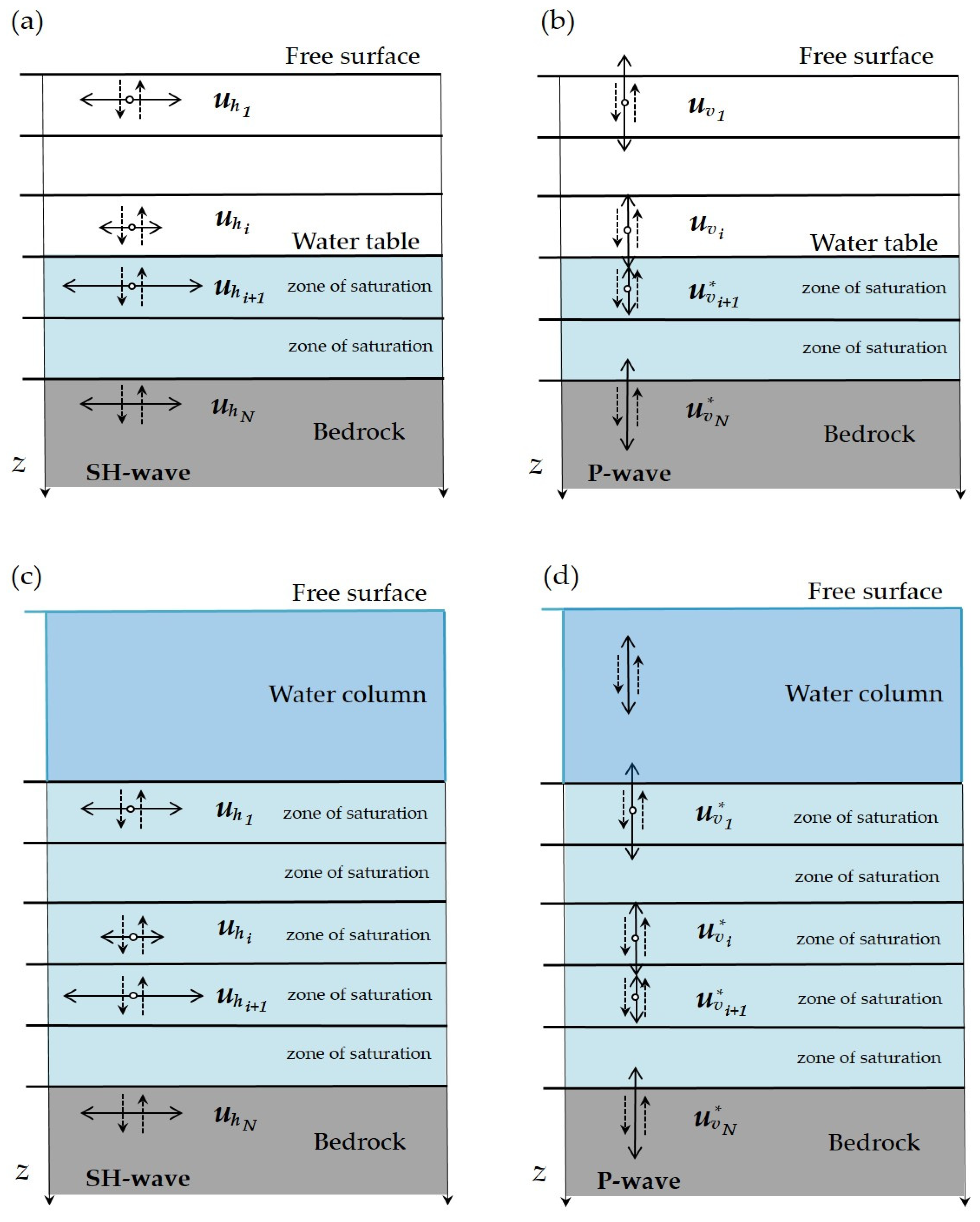
2.1. Scheme of One-Dimensional Horizontally Layered Soil System and Governing Equations of Motion

The study implies one-dimensional vertical propagation of P- and SH-waves in horizontally homogeneous soil layers of infinite horizontal extent. The soil is assumed to be a porous saturated medium. In the general case, the pore fluid may consist of a water, gas mixture, and ice (if we consider the case of a site in the permafrost zone). Figure 1 shows schematically the direction of movement of soil particles relative to the direction of waves propagation through the soil layers in the cases of their occurrence on land (with a certain position of the water table) and in the water area.
Wave equations for propagating shear waves (SH-wave) and compression waves (P-wave) in a horizontally layered system have a simple form:
2 u h z 2 = 1 V S 2   2 u h t 2
2 u v z 2 = 1 V P 2   2 u v t 2
where uh and uv are the horizontal and vertical movement, respectively, as a function of time t and vertical coordinate z, VS and VP are the shear and compression waves velocities, respectively.
The shear wave velocity correlates with the shear modulus, which in turn depends on the stress and strain as follows:
G = ρ b V s 2 = τ h γ h
where G is the shear modulus, ρb is the bulk density, τ h is the horizontal stress, γ h is the horizontal strain.
Similarly, compression wave velocity correlates with constrained modulus, which in turn depends on stress and strain as follows:
M = ρ b V P 2 = τ v γ v
where M is the constrained modulus, τ v is the vertical stress, γ v is the vertical strain.
The relationship between M and G is expressed as follows:
M = 2 G 1 ϑ 1 2 ϑ
where ϑ is the Poisson’s ratio.
In the presence of pore water, the constrained modulus M* differs from that in the absence of underground water M [12,24,27]:
M * = M + K f ϕ
where Kf is the bulk modulus of pore water, is the porosity of the soil.
Thus, the relationship between constrained modulus for saturated soil and compression wave velocity and then, with stress and strain is as follows:
M * = ρ b V P * 2 = τ v * γ v *
where M* is the constrained modulus for saturated soil (i.e., below water table), V P * is the compression waves velocity for saturated soil, τ v * and γ v * are vertical stress and strain for saturated soil, respectively.
Taking into account Formulas (3), (4) and (7), expressions (1) and (2) can be rewritten as follows:
ρ b 2 u h t 2 = ρ b V s 2 2 u h z 2 = G 2 u h z 2
ρ b 2 u v t 2 = ρ b V P 2 2 u v z 2 = M 2 u v z 2
ρ b 2 u v * t 2 = ρ b V P * 2 2 u v * z 2 = M * 2 u v * z 2
where u v * is the vertical movement below the water table.
The derivatives of stresses along z also can be expressed in terms of modules and movements:
τ h z = G γ h z = G 2 u h z 2
τ v z = M γ v z = M 2 u v z 2
τ v * z = M * γ v * z = M * 2 u v * z 2
Combining expressions (8)–(10) and (11)–(13), we can obtain the governing equations of motion:
ρ b 2 u h t 2 = τ h z
ρ b 2 u v t 2 = τ v z
ρ b 2 u v * t 2 = τ v * z
Above, we did not consider the possibility of relative movement of the pore fluid and solid skeleton particles during the passage of seismic waves. However, there is a need to make sure that this approach is correct. To describe the joint relative motion of a solid soil matrix and pore fluid, the Frenkel–Biot theory [23,24] is overwhelmingly used. The theory of poroelastic wave propagation is valid under the assumptions about a bound and isotropic porous medium, the pore scale is much smaller in comparison with the wavelength and small deformations that ensure linear elastic material behavior.
Biot’s equations of motion for an isotropic fluid saturated porous medium are as follows:
ρ b 2 u h t 2 + ρ f 2 w h t 2 = τ h z
p f z + ρ f 2 u h t 2 = Y w h t
w h = ϕ ( u h f u h )
Y = η k ( ω )
where u h f is the horizontal movement of the fluid particles, w h is the horizontal movement of the fluid particles relative to the matrix, ρf is the density of pore fluid, pf is the pore pressure, Y is the viscodynamic operator, η is the dynamic viscosity coefficient of pore fluid, k(ω)—the dynamic permeability (frequency-dependent).
Using Biot’s equations of motion for modeling the site response of soils to shear waves within the seismological frequency range was considered in [1]. For this, assumptions from Gassmann’s theory [25] were used. Gassmann’s theory is based on the assumption that the relative motion of fluid and matrix has a negligible effect on the seismic wave propagation in fluid-saturated soils. Gassmann’s equations are essentially the lower frequency limit of Biot’s more general equations of motion for poroelastic materials. The boundary of the low-frequency range is defined as follows [28]:
f < 0 , 1   η ϕ 2 π k ρ f
where k is the permeability of rock.
In this frequency range, Biot’s theory is in accordance with the conclusions from Gassmann’s theory. In different studies, the value of the cutoff frequency varies. According to [29], the cutoff frequency is within the range of 1–20 kHz. In [30] it is argued that Gassmann’s equations give the most accurate results at frequencies lower than 100 Hz. It follows from this that Gassmann’s theory is well applicable to seismology.
Thus, for modeling seismic waves propagation through porous water-saturated soil layers within the seismology frequency band (lower than 100 Hz) the main assumptions for the elementary volume of porous soil are as follows: firstly, at low frequencies during the passage of the wave, the pore pressure gradients have time to compensate; secondly, there is no relative motion of the fluid and rock matrix, and, thirdly, there is no movement of the pore fluid beyond the elementary soil volume [1]. Taking into account the above assumptions, Biot’s equation of motion (17) take the form (14). For numerical solving of the governing equations of motion, the central difference method was used in accordance with [5].

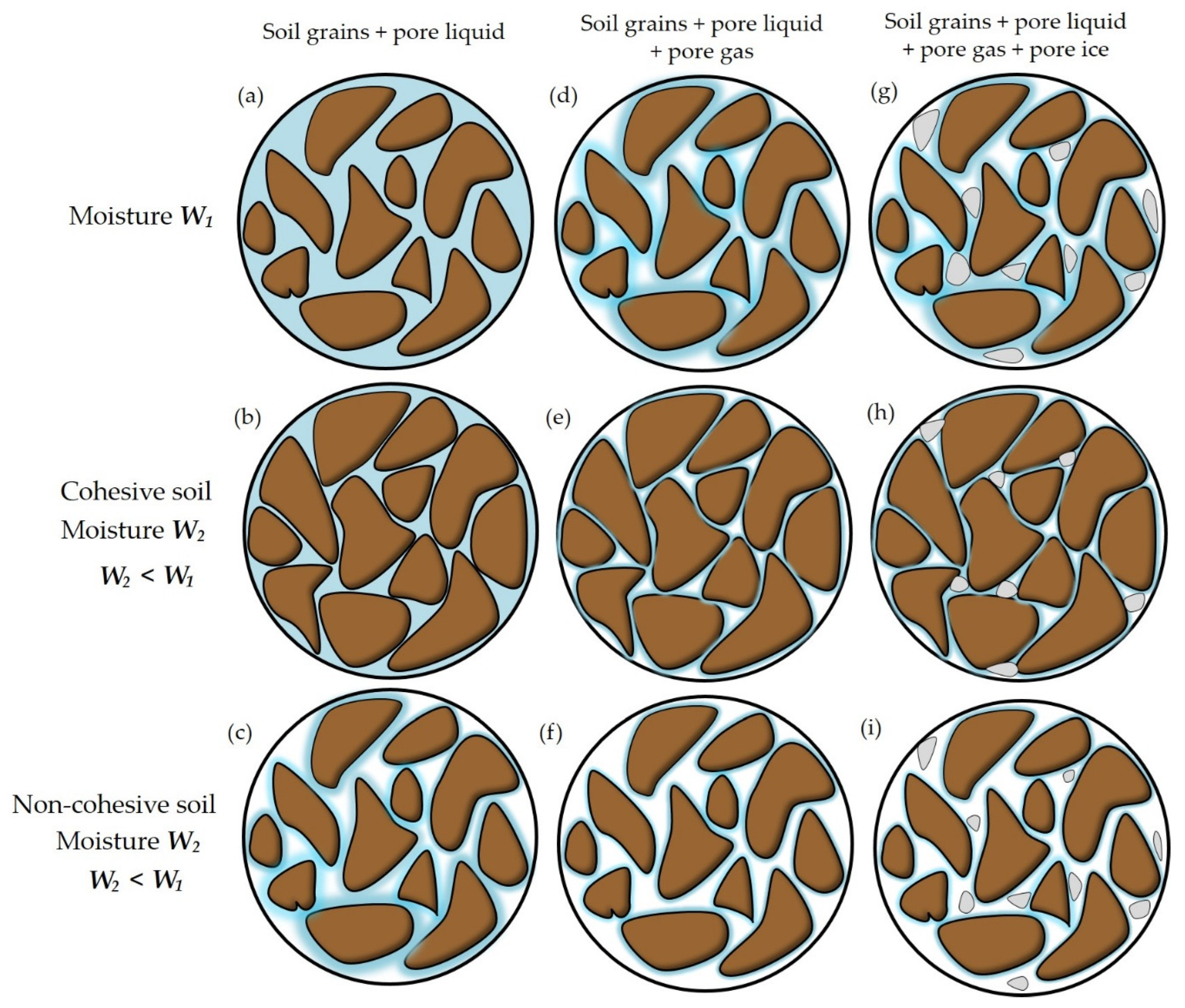
2.2. The Models of Elementary Volume of Saturated Soils

Several variants of the structure of the elementary volume of porous saturated soils are considered (Figure 2), i.e., if the soil consists of: (1) soil matrix and pore water; (2) solid matrix, pore water and gas; (3) solid matrix, pore water, gas and ice. Most sites on land and in water areas are characterized by the second variant of the soil structure. However, the third variant of the soil structure is preferred for sites in permafrost zones.
Loose soils are of particular interest from a geotechnical point of view, including sandy and clayey soils. In the model, the sandy soils were considered non-cohesive and clayey soils—as cohesive. Non-cohesive soils with a solid matrix are characterized by a negligible change in porosity, while fluid saturation of the porous space can vary significantly. For cohesive soils, since their fluid saturation coefficient is close to unity, an increase in moisture leads to an increase in the volume of the pore space [1].
According to Gassman’s theory, since the fluid and solid matrix particles move together, the bulk density of the porous medium can be averaged. If the soil consists only of the solid matrix and pore water, then the averaging takes the following form:
ρ b = ϕ ρ l + ( 1 ϕ ) ρ s
where ρl and ρs are the density of pore liquid (water) and solid grains, respectively.
If the soil consists of a solid matrix, pore water and gas, then the averaging takes the following form:
ρ b = ϕ S g ρ g + ϕ ( 1 S g ) ρ l + ( 1 ϕ ) ρ s
where ρg is the density of pore gas, and Sg is the fraction of gas in pore volume.
If the soil consists of a solid matrix, pore water, gas and ice, then the averaging takes the following form:
ρ b = ϕ S g ρ g + ϕ S i ρ i + ϕ ( 1 S g S i ) ρ l + ( 1 ϕ ) ρ s
where ρi is the density of pore ice, and Si is the fraction of ice in pore volume.
The bulk density can be expressed as a function of the dry density and the moisture coefficient as follows:
ρ b = ρ d r y ( 1 + W )
W = S r e ρ l ρ S
where ρdry is the dry density, W is the moisture coefficient of soil, e is the void ratio, and Sr is the saturation factor (saturated pore volume fraction).

2.3. Nonlinear Hysteretic Model

The typical description of nonlinear soil behavior are models that rely on hysteresis stress-strain relations. With NERA [5], the hysteresis curve is modeled using such parameters as maximum shear modulus Gmax and so-called shear modulus degradation curves G/Gmax(γ) (Figure 3). The IM-model [31,32] implemented in the NERA algorithm assumes the Masing rule [33] and is based on simulating nonlinear hysteretic stress-strain curves using a series of mechanical elements which have different stiffness ki and sliding resistances Ri (R1 < R2 < … < Rn). Initially, the residual stresses in all sliders are equal to zero. During a monotonic loading, slider i yields when the shear stress τ reaches Ri [5].
The results from downhole measurements and from empirical ground motion prediction equations [12,18,34,35] lead to the conclusion that the nonlinear behaviors of vertical and horizontal ground motions differ. Therefore, the modulus reduction and damping curves for the horizontal direction should be modified before applying them to the vertical direction [12], i.e., they should be based on constrained moduli for the cases of unsaturated soil and saturated soil.
The right side of the governing equations of motion (14)–(16) can be written in terms of the tangential modulus:
τ z = τ γ   γ z = H t γ z
where the tangential modulus Ht is [5]:
H t 1 = k 1 ,   i f   0   τ < R 1 H t 2 = ( k 1 1 + k 2 1 ) 1 ,   i f   R 1   τ < R 2 H t n 1 = ( k 1 1 + k 2 1 + + k n 1 1 ) 1 ,   i f   R n 2   τ < R n 1 H t n = ( k 1 1 + k 2 1 + + k n 1 1 + k n 1 ) 1 ,   i f   R n 1   τ < R n 0 ,   i f   τ = R n
The tangential modulus H t i is related to the secant modulus Gi as follows:
H t i = G i + 1 γ i + 1 G i γ i γ i + 1 γ i = G m a x G i + 1 γ i + 1 G i γ i γ i + 1 γ i ,   i = 2 ,   ,   n 1   a n d   H t n = 0 .  
The sliding resistances Ri can be expressed as follows:
R i = G i γ i = G m a x G i γ i ,   i = 1 , ,   n
G i = G i G m a x
Taking into consideration the Equations (5) and (6), the constrained moduli degradation curves for unsaturated soil and for saturated soil, respectively, take the following forms:
M i = M i M m a x = 2 G i 1 ϑ 1 2 ϑ 2 G m a x 1 ϑ 1 2 ϑ = G i
M i * = M i * M m a x * = M i + K f ϕ M m a x + K f ϕ
The damping ratio at horizontal strain γ i can be expressed [5]:
D G i = 2 π   ( 2 A i G i γ i 2 1 ) ,   i = 2 , ,   n
D G 1 = 0
A i = 1 2 j = 2 i ( G j γ j + G j 1 γ j 1 ) ( γ j γ j 1 ) ,   i = 2 , , n
A 1 = 0
where DG is the damping ratio related to horizontal movements.
The damping ratio at vertical strain γ i can be expressed [12]:
D M i = 4 π   1 1 M i [ 1 + ( M i 1 M i ) l n ( M i ) ] 2 π
D M i * = 4 π   1 1 M i * [ 1 + ( M i * 1 M i * ) l n ( M i * ) ] 2 π
where D M and D M * are the damping related to vertical movements for unsaturated soil and saturated soil, respectively.

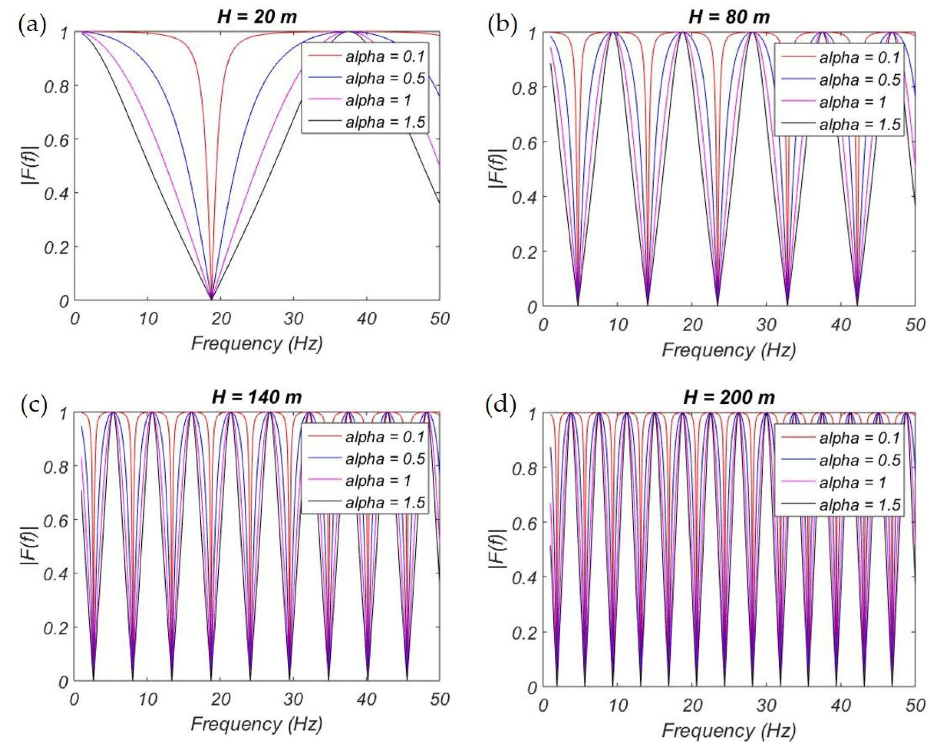
2.4. Effect of Water Column on Incident Plane P-Waves

The ratio of the response of the bottom soil layer with the water column above it to that without a water column [21,36] is as follows:
| F ( f , α ) | = 1 1 + α 2 tan ( π 2 f f 1 r e s )
f n r e s = c w 4 H n
α = ρ w C w ρ s s C s s
where F ( f , α ) is the ratio of the response of the bottom soil layer with the water column above it to that without the water column (reduction spectrum) as a function of frequency f and impedance ratio between water and bottom soil α, f n r e s are the resonant frequencies of P-waves in the water column, n is an odd number, 1,3,5,…, cw is the P-wave velocity in the water layer, H is the thickness of the water column, f 1 r e s is the fundamental resonant frequency, ρw is the density of water, ρss is the density of seafloor soil, Css is the P-wave velocity in seafloor soil (assumed as uniform half space).
Figure 4 shows the reduction spectra | F ( f , α ) | of the vertical component of bottom movements due to the water column of different thickness H above the site and different impedance ratios between seawater and seafloor soil α. In order to simulate this reduction, we suggest sequentially applying a series of band-stop filters to the accelerogram corresponding to the bottom:
a c c _ f i l t i = B u t ( a c c _ f i l t i 1   | [   f i r e s β ;   f i r e s + β ] |   σ ) , f o r   i = 1 , ,   m ;   f 1 r e s     F l b ,   f m r e s     F h b
where But is the operator denoting the application of a digital Butterworth filter of order σ and band-stop frequency range [   f i r e s β ;   f i r e s + β ] , acc_filt0 is the initial accelerogram on the surface of seafloor soil deposits, acc_filti is the filtered accelerogram of iteration i, Flb is the lower representative frequency bound of the initial accelerogram (usually the natural frequency of the accelerometer), Fhb is the upper representative frequency bound of initial accelerogram (usually Nyquist frequency).
Varying the parameters of band-stop frequency range β and the order of the filters σ it is possible to control the depth and width of the spectral peaks corresponding to the resonant frequencies of the P-wave in the water column. Figure 5 shows the correspondence of the target theoretical reduction spectrum due to the water column and frequency response of a complex digital filter designed to simulate it. The following values were used for calculation: cw = 1500 m/s, H = 51 m, α = 0.5, Flb = 1 Hz, Fhb = 50 Hz, σ = 2, β = 1.5 Hz.

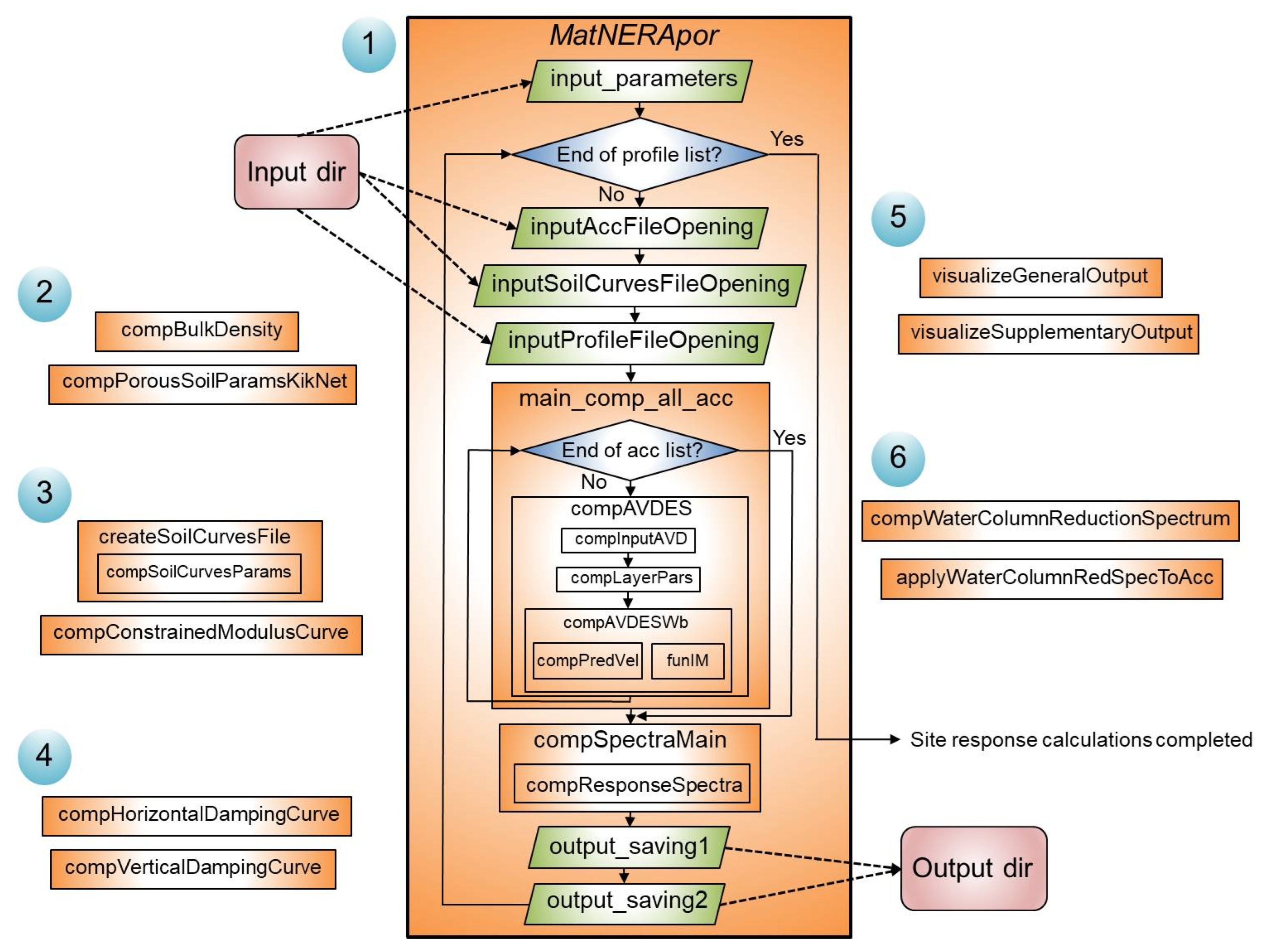
3. Implementation of the Algorithm

The original NERA algorithm [5] was implemented as an Excel add-in and is well documented in the associated user manual. However, the source code is not available. The original implementation of the algorithm had a number of disadvantages: the impossibility of running the program simultaneously for a set of initial signals and soil profiles with subsequent averaging of the obtained spectra, the inability to develop the program, for example, for the case of using other geomechanical models, complicating the structure of soils, considering P-wave propagation, etc.
Therefore, the algorithm presented in this paper was implemented in the Matlab programming environment. The basis is the original NERA algorithm [5]. We added the ability to run calculations both for P- and SH-waves, to calculate the parameters of a porous saturated medium for soil layers and use them in the main algorithm, as well as to obtain constrained moduli reduction curves for the cases above and under the water table. Additionally, we added the ability to run the calculation for a set of input seismic signals, soil profiles, shear and constrained moduli reduction curves with subsequent averaging of the output response spectra. In addition, there is a possibility to obtain the theoretical reduction spectra due to the water column above the sites, simulate this reduction by the set of digital Butterworth bandpass filters and apply them to accelerograms.
The MatNERApor package consists of a set of Matlab scripts and functions. Figure 6 shows the block scheme of the package containing several subsets:
  • Subset 1—a core of earthquake site response computing;
  • Subset 2—a toolkit for calculating the bulk density of porous soil and various parameters of porous soil from velocity profiles for the Kik-net sites;
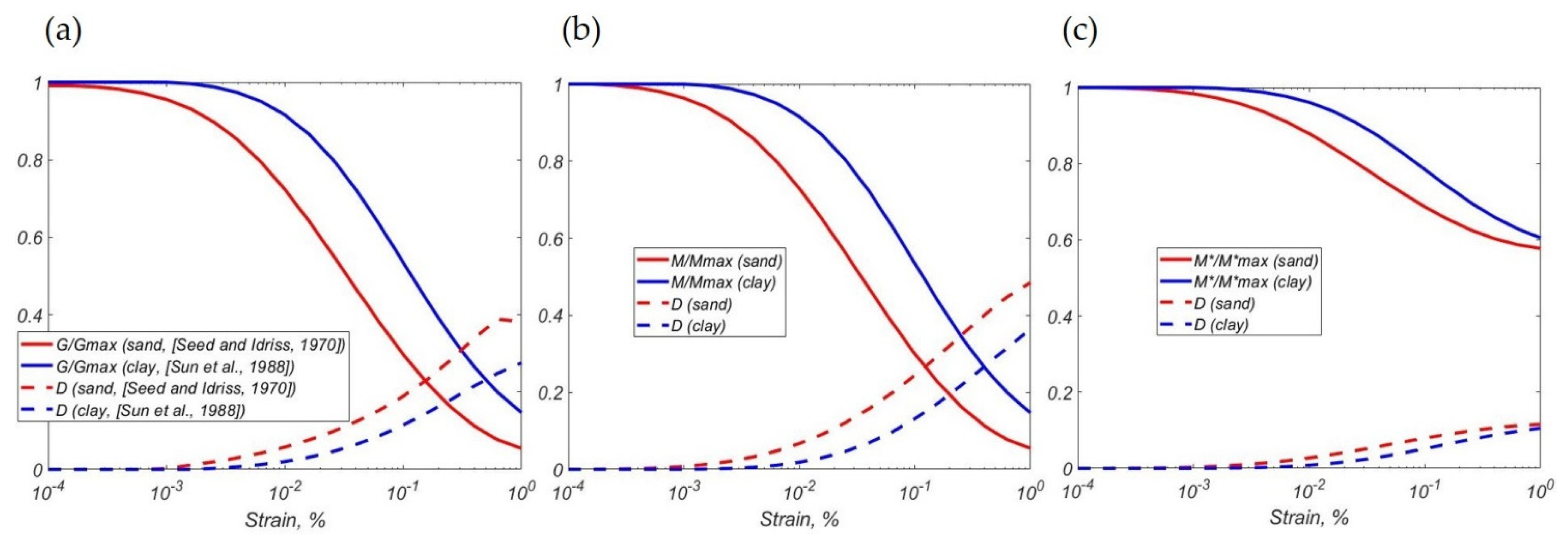
  • Subset 3—a toolkit for calculating constrained moduli degradation curves above and under water table and creating an input file with a set of soil moduli degradation curves;
  • Subset 4—a toolkit for calculating damping curves for P- and SH-wave cases;
  • Subset 5—a toolkit for visualizing general and supplementary output;
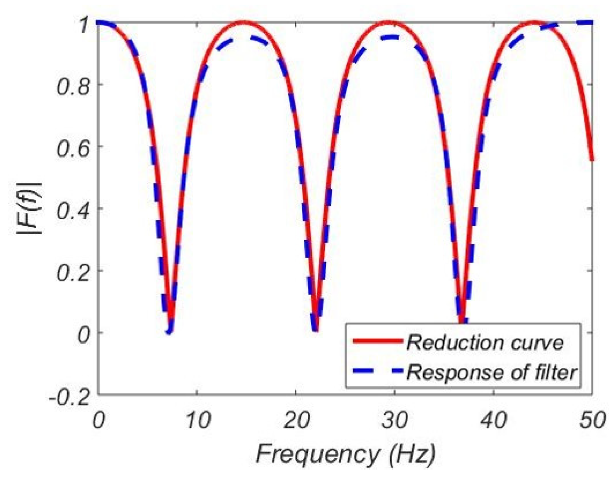
  • Subset 6—a toolkit for calculating theoretical reduction spectra for vertical components due to the water column of different thicknesses above the site, and simulating this reduction by a set of digital Butterworth bandpass filters and applying them to accelerograms.
The MatNERApor package is available in the GitHub repository: https://github.com/ArtWings/MatNERApor.git (Supplementary Materials, accessed on 3 May 2022). In addition, the repository contains a manual describing the purpose of each individual script and function indicated in Figure 6, instructions for running the program, as well as a description of the format of input and output data.

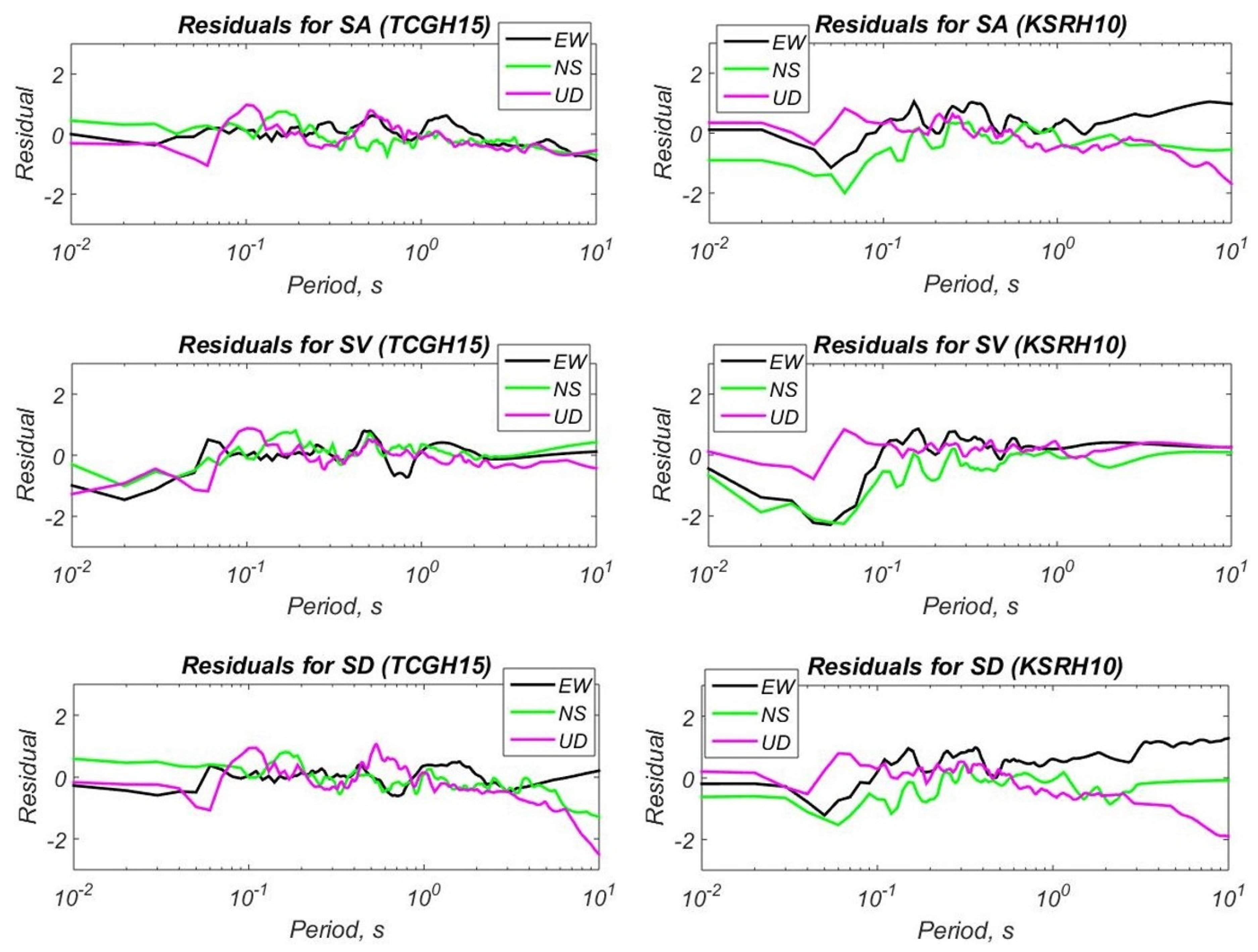
4. Approbation of the Algorithm with the Kik-Net Vertical Arrays Data

To verify the modeling results, the records of vertical seismic arrays of the Kik-net network [26] were used. Figure 7 shows the VP and VS velocity profiles at TCGH15 and KSRH10 sites. The TCGH15 site is characterized by sandy soils lying on the bedrock at a depth of 22 m. The KSRH10 site is characterized by clayey soils lying on the bedrock at a depth of 36 m [37].
For most cases, only velocity profiles are available in the database [26]. Other geotechnical parameters were calculated according to various equations (Table 1 and Table 2). The bulk density can be calculated as a function of the P-wave velocity [38] or as a function of the S-wave velocity [39]. Figure 7 shows that at a certain depth there can be a sharp increase in VP with a relatively small increase in VS. Such a horizon can be interpreted as the level of groundwater. The bedrock is characterized by a significant increase in both VP and VS. In accordance with the accepted model of the elementary volume of soils with different moisture content (Figure 2), the dependences of density on VP are better suited for finding the bulk density of non-cohesive soils, since an increase in moisture of such soils should lead to an increase in bulk density. Conversely, to find the bulk density of cohesive soils, the dependences of density on VS are better suited since an increase in moisture of such soils should lead to a smaller change in density or to its decrease.
Two earthquakes were chosen to model the site response as they resulted in approximately the same PGA at both sites (~60 Gal):
(1)
Mw = 5.7, origin time 6 October 2004 14:40:38 UTC (for TCGH15 site) [40];
(2)
Mw = 5.2, origin time 10 May 2008 18:24:02 UTC (for KSRH10 site) [40].
Figure 8 shows degradation curves of shear modulus (from literature), constrained moduli above the water table and under the water table (calculated) and corresponding damping ratio curves used for modeling the responses for TCGH15 and KSRH10 Kik-net sites. We used the shear modulus degradation curves from [41] for sandy sites, from [42] for clayey sites and from [2] for stiff bedrock.
Figure 9 and Figure 10 show a comparison of the response spectra modeled by MatNERApor and recorded accelerograms on the surface of soil layers at TCGH15 and KSRH10 sites, respectively. Calculations were carried out for all three components of records. It can be seen that the simulation results basically correspond to real records.
Modeling accuracy can be assessed by using the residuals as follows [12]:
R S A ( T ) = ln [ S A ( T ) ] r e c o r d l n [ S A ( T ) ] m o d e l R S V ( T ) = ln [ S V ( T ) ] r e c o r d l n [ S V ( T ) ] m o d e l R S D ( T ) = ln [ S D ( T ) ] r e c o r d l n [ S D ( T ) ] m o d e l
where [ S A ( T ) ] r e c o r d ,   [ S V ( T ) ] r e c o r d ,   [ S D ( T ) ] r e c o r d are spectral acceleration, velocity and displacement of the record for period T, [ S A ( T ) ] m o d e l ,   [ S V ( T ) ] m o d e l ,   [ S D ( T ) ] m o d e l are spectral acceleration, velocity and displacement of the modeled accelerograms for period T.
Figure 11 shows the residuals of response spectra of modeled and recorded accelerograms calculated for the surface of soil layers at Kik-net sites TCGH15 and KSRH10. The obtained residuals for the TCGH15 site turned out to be on average smaller than for the KSRH10 site. However, this does not apply to the vertical components. Moreover, the residuals for the vertical component for the KSRH10 site are smaller than for the horizontal components, especially in the spectral range T < 0.1 s. For the TCGH15 site, the residuals of the horizontal and vertical components are mostly similar. It should also be noted that, for spectral displacements, the residuals noticeably increase in the spectral range T > 3 for both sites.

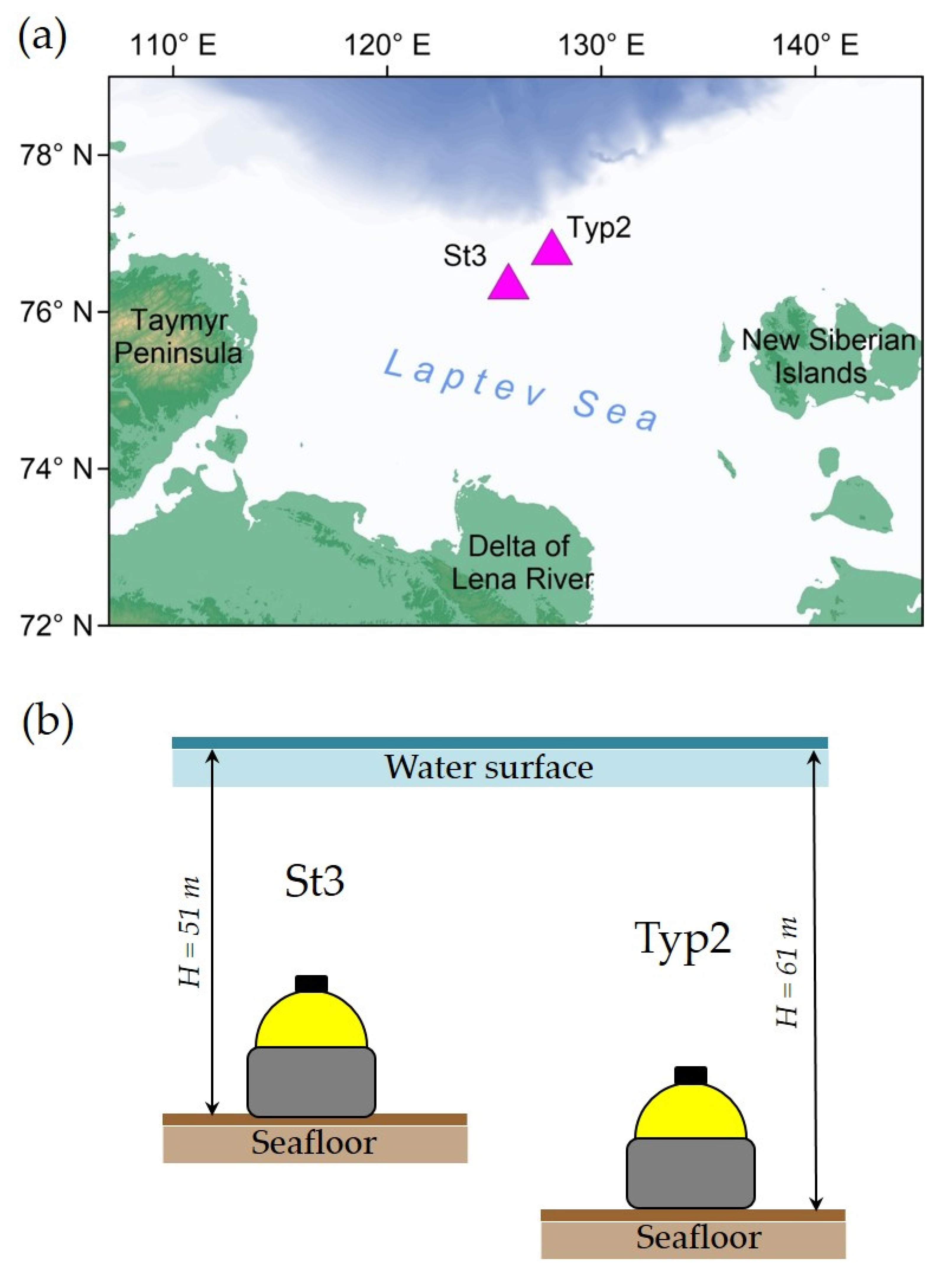
5. Calculation of Water Column Reduction Spectra Using the OBS Records Obtained in the Arctic

Analysis of the seismic response of soils for water areas has peculiarities. Some studies based on the analysis of seismic records obtained on the seafloor show that the vertical component of seafloor ground motions is significantly lower than that of on-land ground motions near the P-wave resonant frequencies caused by the water column above the seismograph [20,21,22]. To demonstrate this effect, records of local earthquakes obtained by ocean bottom seismographs in the Laptev Sea in 2019–2020 were used.
Figure 12 shows the location of two OBSs deployed during the AMK-78 cruise (October 2019) and dismantled during the AMK-82 cruise (October 2020) in the Laptev Sea aboard the R/V Akademik Mstislav Keldysh. A series of scientific cruises to the Laptev Sea and East-Siberian Sea were organized by the V.I. Ilichov Pacific Oceanological Institute of the Far Eastern Branch of the Russian Academy of Sciences and the IO RAS with the participation of a number of other institutions. Since 2018, the program of seismological research has been included in these expeditions and has aimed to obtain the seismic and seismotectonic characteristics of the Laptev Sea region in the context of the relationship of the tectonic processes with the discharge of bubble methane from the bottom by registering local microearthquakes, remote teleseismic events and ambient seismic noise on the shelf and the continental slope of the Laptev Sea [45,46].
The two OBSs were located near, but not exactly within, large methane seep fields [14]. The central part of the outer Laptev Sea shelf is characterized by scattered areas of sub-bottom permafrost and taliks [47,48]. The soil layers in such areas have a multiphase structure: solid soil grains, pore water, ice and gas mixture.
It turned out that the OBS recording capabilities on the Arctic shelf and the upper slope are highly dependent on the level of ambient seismic noise, which, in turn, is influenced by the wind waves. A strong noise level, at least in the autumn ice-free time period, practically leads to the impossibility of obtaining high-quality records of earthquakes. Ice-cover smooths out wind waves and significantly reduces noise levels [45,46]. In the ice-covered time period, the OBS deployments resulted in a significant number of signals from both large remote and weak local earthquakes in a broad frequency range.
Figure 13 shows the V/H curves, i.e., the ratio of the FFT spectra of the vertical to the horizontal component, for 10 local earthquakes of similar strength and epicentral distance, obtained at two points (St3 and Typ2—see Figure 12) located at a considerable distance from each other.
A clear drop in the V/H curves is seen at frequencies of 3–10 Hz and for both OBSs. The depth of the sea above the St3 and Typ2 sites is 51 and 61 m, respectively. The theoretical estimate of the resonant frequencies of P-waves by Equation (37) is 5–7 Hz for these depths. In addition, the theoretical reduction spectra due to the water column above the sites are shown in Figure 13. The following values were used for calculation of theoretical reduction spectra by Equations (36) and (37): cw = 1500 m/s, H = 51 m, α = 2 (Figure 13a); cw = 1500 m/s, H = 61 m, α = 1 (Figure 13b). The speed of sound in water cw is assumed to be typical. The thicknesses of water column H for both sites were obtained from ship echo sounder data. The values of impedance ratio between water and bottom soil α were chosen so that the main peak widths of the theoretical reduction spectra corresponded to those obtained on real records. It should be noted that this method of impedance ratio selection can be considered as an additional method for determining the impedance of submarine surface soils for engineering purposes. Figure 13 demonstrates a good agreement between recorded and theoretical spectral reduction for both sites.

6. Conclusions

Summarizing the above, we can formulate the following main conclusions:
(1)
The algorithm MatNERApor and its Matlab implementation were introduced for numerical modeling of the nonlinear response of porous saturated soil deposits to P- and SH-waves vertical propagation. The presented algorithm is based on the NERA algorithm, but develops significantly, expanding its applicability to the cases of a porous saturated soil structure, propagation of P-waves instead of SH-waves and occurrence of soil deposits in the water area. In addition, many shortcomings of the software implementation of the original algorithm have been overcome. We added the ability to run the calculation for a set of input seismic signals, soil profiles, shear and constrained moduli reduction curves with subsequent averaging of the output response spectra. The source code can be further developed.
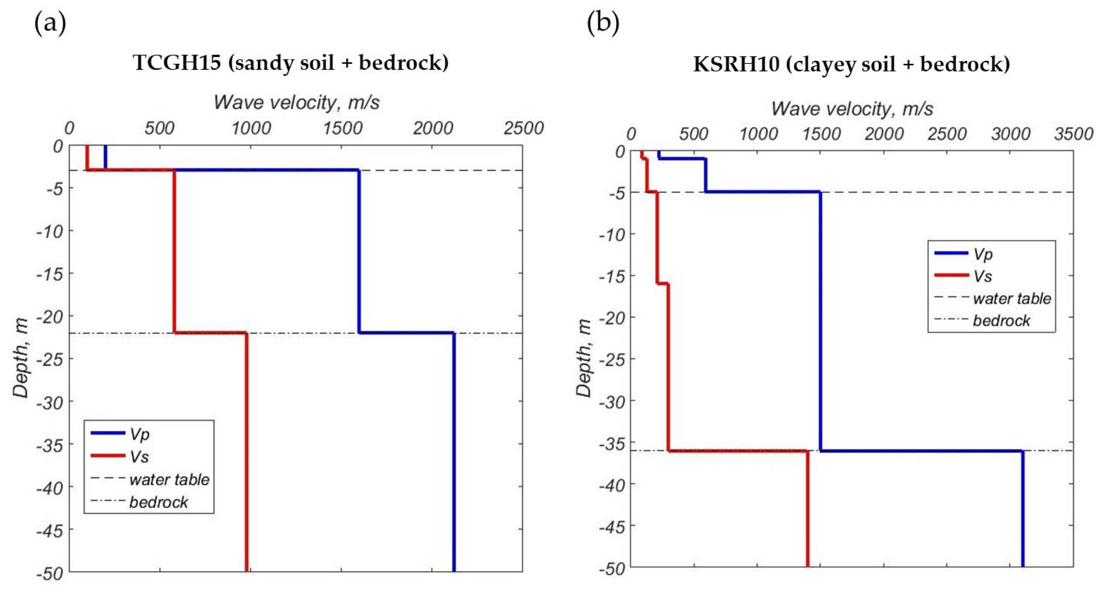
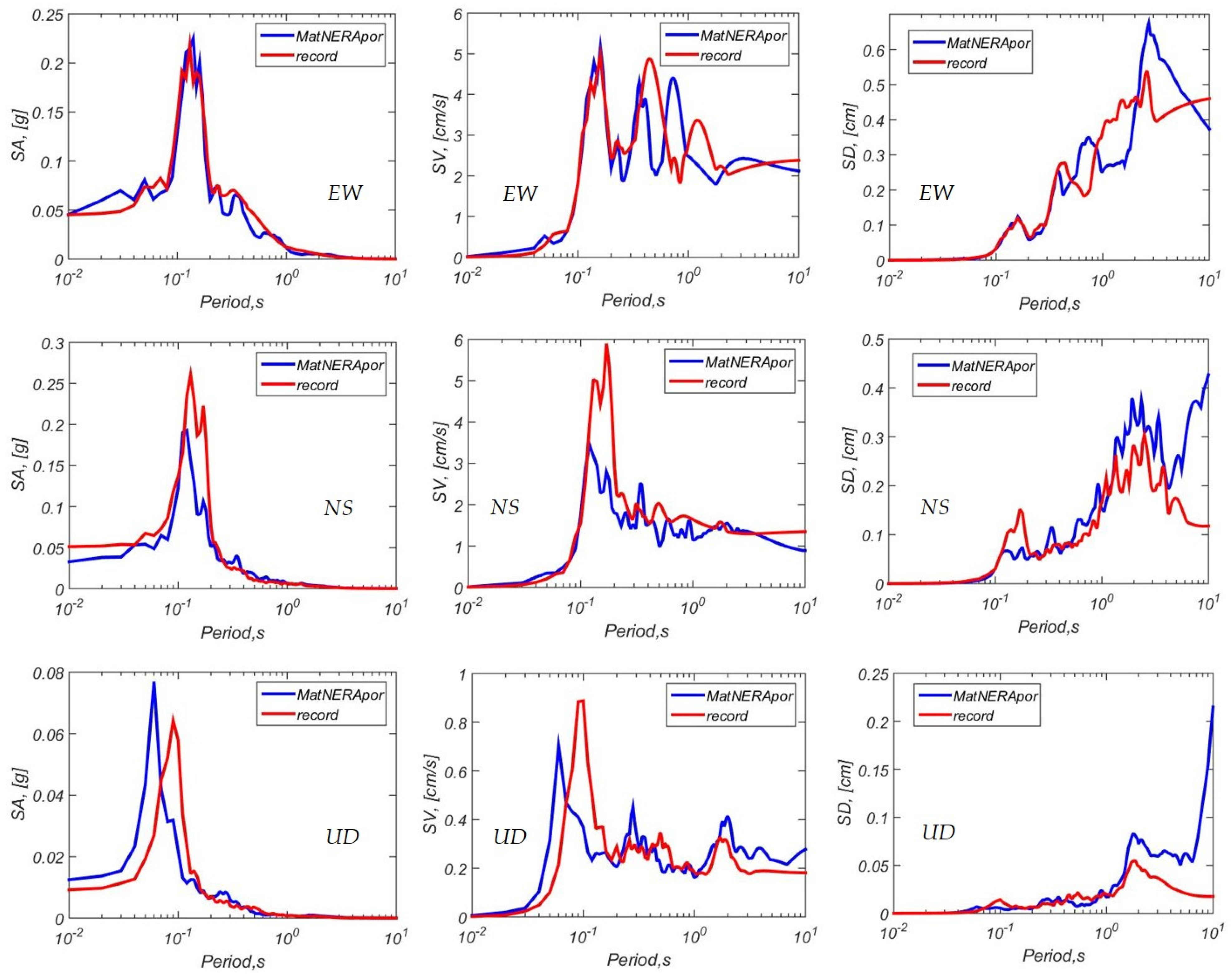
(2)
The package was tested and verified using the records at two sites of the Kik-net network: the TCGH15 site is characterized by sandy soils lying on the bedrock, and the KSRH10 site is characterized by clayey soils. The effect of the water column on the reduction of vertical motion spectra was demonstrated using the records of local earthquakes obtained by ocean bottom seismographs in the Laptev Sea in 2019–2020. The results of the calculations showed good agreement with the data obtained from real seismic records, which justifies the correctness of the theoretical basis of the presented algorithm and its software implementation.
(3)
The MatNERApor package has significant prospects for practical use. This is especially actual for sites located in the water area within the zones of continuous or sparse permafrost, as well as the massive release of bubble gas from bottom sediments, such as the Arctic shelf of Eastern Siberia. In this case, it is especially important to consider the complex structure of marine soils, i.e., their saturation with water, gas mixture and ice.

Supplementary Materials

The MatNERApor package and the manual are available in GitHub repository: https://github.com/ArtWings/MatNERApor.git (accessed on 3 May 2022).

Author Contributions

Conceptualization, A.A.K.; methodology, A.A.K.; software, A.A.K., E.A.R., M.A.N.; validation, A.A.K.; formal analysis, A.A.K.; investigation, A.A.K., S.A.K., E.A.R., M.A.N.; data curation, A.A.K., L.I.L., I.P.S.; writing—original draft preparation, A.A.K.; writing—review and editing, all authors; visualization, A.A.K.; supervision, A.A.K., L.I.L., I.P.S.; project administration, A.A.K., K.A.R., L.I.L., I.P.S.; funding acquisition, A.A.K., O.S.S., K.A.R., I.P.S. All authors have read and agreed to the published version of the manuscript.

Funding

This work was financially supported by the Russian Science Foundation, project no. 20-77-00034 (developing of the site response algorithm and its approbation); Russian Foundation for Basic Research, project no. 20-05-00533 (collecting and processing the ocean bottom seismograph records, calculating spectral ratios of earthquake signals); the Russian State Assignment, project no. FMWE-2021-0004 (a review of publications on modeling the earthquake site response); the Ministry of Science and Higher Education of the Russian Federation, project no. 1021052204209-8 and no. FMWE-2021-0011 (discussion of the results in the broad interdisciplinary context, text editing); the Russian President Grant for young scientists, project no. MK-45.2022.1.5 (study of earthquake site response in context of its relation to endogenous geological hazards); the Russian Science Foundation, project no. 21-77-30001 (developing of the models of porous soil structure, typical for marine soils in the area of active methane seepage from seafloor); the Ministry of Science and High Education of the Russian Federation, project no. 075-15-2020-928, HSE (study of the seismic load effect on sub-bottom permafrost condition).

Institutional Review Board Statement

Not applicable.

Informed Consent Statement

Not applicable.

Data Availability Statement

Not applicable.

Conflicts of Interest

The authors declare no conflict of interest.

References

  1. Krylov, A.A.; Alekseev, D.A.; Kovachev, S.A.; Radiuk, E.A.; Novikov, M.A. Numerical Modeling of Nonlinear Response of Seafloor Porous Saturated Soil Deposits to SH-Wave Propagation. Appl. Sci. 2021, 11, 1854. [Google Scholar] [CrossRef]
  2. Schnabel, P.B.; Lysmer, J.; Seed, H.B. SHAKE: A Computer Program for Earthquake Response Analysis of Horizontally Layered Sites; Report No. UCB/EERC-28 -72/12; Earthquake Engineering Research Center, University of California: Berkeley, CA, USA, 1972; 102p. [Google Scholar]
  3. Bardet, J.P.; Ichii, K.; Lin, C.H. EERA: A computer program for Equivalent Linear Earthquake Site Response Analysis of Layered Soils Deposits; University of Southern California: Los Angeles, CA, USA, 2000; 38 p. [Google Scholar]
  4. Kottke, A.R.; Rathje, E.M. Technical Manual for Strata; PEER Report 2008/10; Pacifc Earthquake Engineering Research Center College of Engineering, University of California: Berkeley, CA, USA, 2008; 100p. [Google Scholar]
  5. Bardet, J.P.; Tobita, T. NERA, A Computer Program for Nonlinear Earthquake Site Response Analyses of Layered Soil Deposits; University of Southern California: Los Angeles, CA, USA, 2001; 44p. [Google Scholar]
  6. Hashash, Y.M.A.; Musgrove, M.I.; Harmon, J.A.; Ilhan, O.; Xing, G.; Numanoglu, O.; Groholski, D.R.; Phillips, C.A.; Park, D. DEEPSOIL 7, User Manual; Board of Trustees of University of Illinois at Urbana-Champaign: Urbana, IL, USA, 2020; 170p, Available online: http://deepsoil.cee.illinois.edu/Publications.html (accessed on 22 February 2022).
  7. Matasovic, N. Seismic Response of Composite Horizontally-Layered Soil Deposits. Ph.D. Thesis, University of California, Los Angeles, CA, USA, 1993. [Google Scholar]
  8. Kramer, S.L.; Paulsen, S.B. Practical Use of Geotechnical Site Response Models. In Proceedings of the International Workshop on Uncertainties in Nonlinear Soil Properties and Their Impact on Modeling Dynamic Soil Response, University of California, Berkeley, Richmond, CA, USA, 18–19 March 2004; p. 10. [Google Scholar]
  9. Kramer, S.L. Geotechnical Earthquake Engineering; Prentice Hall: Upper Saddle River, NJ, USA, 1996; 653p. [Google Scholar]
  10. Papazoglou, A.J.; Elnashai, A.S. Analytical and field evidence of the damaging effect of vertical earthquake ground motion. Earthq. Eng. Struct. Dyn. 1996, 25, 1109–1137. [Google Scholar] [CrossRef]
  11. Gülerce, Z.; Abrahamson, N.A. Vector-valued probabilistic seismic hazard assessment for the effects of vertical ground motions on the seismic response of highway bridges. Earthq. Spectra 2010, 26, 999–1016. [Google Scholar] [CrossRef]
  12. Tsai, C.-C.; Lui, H.-W. Site response analysis of vertical ground motion in consideration of soil nonlinearity. Soil Dyn. Earthq. Eng. 2017, 102, 124–136. [Google Scholar] [CrossRef]
  13. Yuan, R.-M.; Tang, C.-L.; Deng, Q.-H. Effect of the acceleration component normal to the sliding surface on earthquake-induced landslide triggering. Landslides 2015, 12, 335–344. [Google Scholar] [CrossRef]
  14. Shakhova, N.; Semiletov, I.; Sergienko, V.; Lobkovsky, L.; Yusupov, V.; Salyuk, A.; Salomatin, A.; Chernykh, D.; Kosmach, D.; Panteleev, G.; et al. The East Siberian Arctic Shelf: Towards further assessment of permafrost-related methane fluxes and role of sea ice. Phil. Trans. R. Soc. A. 2015, 373, 20140451. [Google Scholar] [CrossRef]
  15. Shakhova, N.; Semiletov, I.; Gustafsson, Ö.; Sergienko, V.; Lobkovsky, L.; Dudarev, O.; Tumskoy, V.; Grigoriev, M.; Mazurov, A.; Salyuk, A.; et al. Current rates and mechanisms of subsea permafrost degradation in the East Siberian Arctic Shelf. Nat. Commun. 2017, 8, 15872. [Google Scholar] [CrossRef]
  16. Shakhova, N.; Semiletov, I.; Chuvilin, E. Understanding the Permafrost–Hydrate System and Associated Methane Releases in the East Siberian Arctic Shelf. Geosciences 2019, 9, 251. [Google Scholar] [CrossRef] [Green Version]
  17. Towhata, I. Geotechnical Earthquake Engineering; Springer: Berlin/Heidelberg, Germany, 2008; 684p. [Google Scholar] [CrossRef]
  18. Stewart, J.P.; Boore, D.M.; Seyhan, E.; Atkinson, G.M. NGA-West2 equations for predicting vertical-component PGA, PGV, and 5%-damped PSA from shallow crustal earthquakes. Earthq. Spectra 2016, 32, 1005–1031. [Google Scholar] [CrossRef]
  19. Beresnev, I.A.; Nightingale, A.M.; Silva, W.J. Properties of Vertical Ground Motions. Bull. Seismol. Soc. Am. 2002, 92, 3152–3164. [Google Scholar] [CrossRef]
  20. Li, C.; Hao, H.; Li, H.; Bi, K.; Chen, B. Modeling and Simulation of Spatially Correlated Ground Motions at Multiple Onshore and Offshore sites. J. Earthq. Eng. 2017, 21, 359–383. [Google Scholar] [CrossRef] [Green Version]
  21. Diao, H.; Hu, J.; Xie, L. Effect of seawater on incident plane P and SV waves at ocean bottom and engineering characteristics of offshore ground motion records off the coast of southern California, USA. Earthq. Eng. Eng. Vib. 2014, 13, 181–194. [Google Scholar] [CrossRef]
  22. Boore, D.M.; Smith, C.E. Analysis of earthquake recordings obtained from the seafloor earthquake measurement system (SEMS) instruments deployed off the coast of Southern California. Bull. Seismol. Soc. Am. 1999, 89, 260–274. [Google Scholar] [CrossRef]
  23. Frenkel, J. On the Theory of Seismic and Seismoelectric Phenomena in a Moist Soil. J. Phys. 1994, 111, 230–241, Republished in: J. Eng. Mech., 2005, 131, 879‒887. [Google Scholar] [CrossRef] [Green Version]
  24. Biot, M. Theory of propagation of elastic waves in a fluid-saturated porous solid. J. Acoust. Soc. Am. 1956, 28, 168–191. [Google Scholar] [CrossRef]
  25. Gassmann, F. Über die Elastizität poröser Medien. Viertel Nat. Ges. Zürich 1951, 96, 1–23. [Google Scholar]
  26. National Research Institute for Earth Science and Disaster Resilience (NIED). Available online: https://www.kyoshin.bosai.go.jp/ (accessed on 20 November 2021).
  27. Bardet, J.P. The damping of saturated poroelastic soils during steady-state vibrations. Appl. Math. Comput. 1995, 67, 3–31. [Google Scholar] [CrossRef]
  28. White, J.E. Underground Sound: Application of Seismic Waves. Methods Geochem. Geophys. 1983, 18, 253. [Google Scholar] [CrossRef]
  29. Avseth, P.; Mukerji, T.; Mavko, G. Quantitative Seismic Interpretation: Applying Rock Physics Tools to Reduce Interpretation Risk; United Kingdom at the University Press: Cambridge, UK, 2005; 359p. [Google Scholar] [CrossRef]
  30. Mavko, G.; Mukerji, T.; Dvorkin, J. The Rock Physics Handbook: Tools for Seismic Analysis of Porous Media; United States of America by Cambridge University Press: New York, NY, USA, 2009; 511p. [Google Scholar] [CrossRef]
  31. Iwan, W.D. On a class of models for the yielding behavior of continuous and composite systems. J. Appl. Mech. ASME 1967, 34, 612–617. [Google Scholar] [CrossRef]
  32. Mróz, Z. On the description of anisotropic workhardening. J. Mech. Phys. Solids 1967, 15, 163–175. [Google Scholar] [CrossRef]
  33. Masing, G. Eigenspannungen and verfertigung beim messing. In Proceedings of the 2nd International Congress of Applied Mechanics, Zurich, Switzerland, 12–17 September 1926; pp. 332–335. [Google Scholar]
  34. Elgamal, A.; He, L.C. Vertical earthquake ground motion records: An overview. J. Earthq. Eng. 2004, 8, 663–697. [Google Scholar] [CrossRef]
  35. Bozorgnia, Y.; Campbell, K.W. Vertical Ground Motion Model Using NGA-West2 database. Earthq. Spectra 2015, 32, 150414082519000. [Google Scholar] [CrossRef]
  36. Crouse, C.B.; Quilter, J. Seismic Hazard Analysis and Development of Design Spectra for Maul A Platform. In Proceedings of the Pacific Conference on Earthquake Engineering, Auckland, New Zealand, 20–23 November 1991; Vol. III, pp. 137–148. [Google Scholar]
  37. Bajaj, K.; Anbazhagan, P. Identification of Shear Modulus Reduction and Damping Curve for Deep and Shallow Sites: Kik-Net Data. J. Earthq. Eng. 2021, 25, 2668–2696. [Google Scholar] [CrossRef]
  38. Gardner, G.H.F.; Gardner, L.W.; Gregory, A.R. Formation velocity and density—The diagnostic basics for stratigraphic traps. Geophysics 1974, 39, 770–780. [Google Scholar] [CrossRef] [Green Version]
  39. Anbazhagan, P.; Uday, A.; Moustafa, S.S.R.; Al-Arifi, N.S.N. Correlation of densities with shear wave velocities and SPT N values. J. Geophys. Eng. 2016, 13, 320–341. [Google Scholar] [CrossRef] [Green Version]
  40. IRIS Wilber 3 system. Available online: https://ds.iris.edu/wilber3/ (accessed on 22 January 2022).
  41. Seed, H.B.; Idriss, I.M. Soil Moduli and Damping Factors for Dynamic Response Analysis; Report No. UCB/EERC-70/10; Earthquake Engineering Research Center, University of California: Berkeley, CA, USA, 1970; 48p. [Google Scholar]
  42. Sun, J.I.; Golesorkhi, R.; Seed, H.B. Dynamic Moduli and Damping Ratios for Cohesive Soils; Report No. UCB/EERC-88/15; Earthquake Engineering Research Center, University of California: Berkeley, CA, USA, 1988; 42p. [Google Scholar]
  43. Presnov, O.M. Mekhanika Gruntov: Uchebno-Metodicheskoe Posobie [Soil Mechanics: Teaching Aid]; Krasnoyarsk Siberian Federal University: Krasnoyarsk, Russia, 2012; 67p. (In Russian) [Google Scholar]
  44. Lomtadze, V.D. Inzhenernaya Geologiya. In Inzhenernaya Petrologiya [Engineering Geology. Engineering Petrology], (In Russian), 2nd ed.; USSR: Nedra, Leningrad, 1984; 509p. (In Russian) [Google Scholar]
  45. Krylov, A.A.; Ivashchenko, A.I.; Kovachev, S.A.; Tsukanov, N.V.; Kulikov, M.E.; Medvedev, I.P.; Ilinskiy, D.A.; Shakhova, N.E. The Seismotectonics and Seismicity of the Laptev Sea Region: The Current Situation and a First Experience in a Year-Long Installation of Ocean Bottom Seismometers on the Shelf. J. Volcanolog. Seismol. 2020, 14, 379–393. [Google Scholar] [CrossRef]
  46. Krylov, A.A.; Egorov, I.V.; Kovachev, S.A.; Ilinskiy, D.A.; Ganzha, O.Y.; Timashkevich, G.K.; Roginskiy, K.A.; Kulikov, M.E.; Novikov, M.A.; Ivanov, V.N.; et al. Ocean-Bottom Seismographs Based on Broadband MET Sensors: Architecture and Deployment Case Study in the Arctic. Sensors 2021, 21, 3979. [Google Scholar] [CrossRef]
  47. Bogoyavlensky, V.I.; Kishankov, A.V.; Kazanin, A.G. Permafrost, Gas Hydrates and Gas Seeps in the Central Part of the Laptev Sea. Dokl. Earth Sci. 2021, 500, 766–771. [Google Scholar] [CrossRef]
  48. Bogoyavlensky, V.; Kishankov, A.; Kazanin, A.; Kazanin, G. Distribution of permafrost and gas hydrates in relation to intensive gas emission in the central part of the Laptev Sea (Russian Arctic). Mar. Pet. Geol. 2022, 138, 105527. [Google Scholar] [CrossRef]
Figure 1. One-dimensional horizontally layered system of porous saturated soils and its spatial discretization in the case of vertically propagated waves: (a) a shear wave (on-land site), (b) a compression wave (on-land site), (c) a shear wave (site in water area), (d) a compression wave (site in water area).
Applsci 12 04614 g001
Figure 2. Schematic representation of the elementary volume of cohesive and non-cohesive soil with different moisture values and different soil structure: (ac)—if soil consists of soil grains and pore liquid (water); (df)—if soil consists of soil grains, pore liquid and gas; (gi)—if soil consists of soil grains, pore liquid, gas and ice.
Applsci 12 04614 g002
Figure 3. Hysteresis curve (a), schematic representation of stress-strain model introduced by [31,32] (b), degradation curves of shear modulus G/Gmax (γ), constrained moduli above water table M/Mmax (γ) and under water table M*/M*max (γ) and corresponding damping ratio curves DG(γ), DM(γ), DM*(γ) (c).
Applsci 12 04614 g003
Figure 4. Reduction spectra for vertical component of bottom movements due to the water column of different thicknesses (H) above the site: (a) – H = 20 m, (b) – H = 80 m, (c) – H = 140 m, (d) – H = 200 m (alpha—impedance ratio between seawater and seafloor soil).
Applsci 12 04614 g004
Figure 5. Target theoretical reduction spectrum due to the water column and frequency response of complex digital filter designed to simulate it.
Applsci 12 04614 g005
Figure 6. Block-scheme of MatNERApor Matlab package for numerical modeling of nonlinear response of porous saturated soil deposits to seismic body waves propagation. Numbers in blue circles—subsets of the package (see description in text).
Applsci 12 04614 g006
Figure 7. Velocity profiles at sites TCGH15 (a) and KSRH10 (b) of the Kik-net network.
Applsci 12 04614 g007
Figure 8. Degradation curves of shear modulus G/Gmax (γ) (a), constrained moduli above water table M/Mmax (γ) (b) and under water table M*/M*max (γ) (c) and corresponding damping ratio curves D(γ) (c) used for modeling the responses for TCGH15 and KSRH10 Kik-net sites.
Applsci 12 04614 g008
Figure 9. Comparison of response spectra (damping 5%) of modeled and recorded accelerograms (components EW, NS, UD; spectral acceleration—SA, spectral velocity—SV, spectral displacement—SD) calculated for the surface of soil layers at Kik-net site TCGH15.
Applsci 12 04614 g009
Figure 10. Comparison of response spectra (damping 5%) of modeled and recorded accelerograms (components EW, NS, UD; spectral acceleration—SA, spectral velocity—SV, spectral displacement—SD) calculated for the surface of soil layers at Kik-net site KSRH10.
Applsci 12 04614 g010
Figure 11. Residuals of response spectra (damping 5%) of modeled and recorded accelerograms (components EW, NS, UD; spectral acceleration—SA, spectral velocity—SV, spectral displacement—SD) calculated for the surface of soil layers at Kik-net sites TCGH15 and KSRH10.
Applsci 12 04614 g011
Figure 12. (a)—OBS deployment sites on the outer shelf of the Laptev sea (operation time period: October 2019—January 2020); (b)—schematic view of the OBS deployed in the Laptev sea with indication of sea depths.
Applsci 12 04614 g012
Figure 13. V/H spectral ratio curves of 10 local earthquake signals obtained at St3 site (a), at Typ2 site (b) and corresponding theoretical reduction spectra due to the water column above the sites. Gray lines—the earthquakes FFT spectral ratio curves; red line—the average curve for the FFT spectral ratios; blue line—the theoretical reduction spectra.
Applsci 12 04614 g013
Table 1. Geotechnical parameters (initial and calculated) at the TCGH15 sandy site of the Kik-net network.
Source: [26]Calculated According to [38]Calculated According to [39]Source: [43,44]Calculated by Equations (22) and (25)
Depth to Top of Layer (m)Vp,
(m/s)
Vs,
(m/s)
ρ bulk = f(Vp),
(kg/m3)
ρ bulk = f(Vs),
(kg/m3)
ρ dry = f(Vs),
(kg/m3)
ρS,
(kg/m3)
W = f(ρ, ρ dry)ϕ = f(ρ dry, ρS)
02001001164137712722.660.080.52
316005801958218217862.660.220.33
22 *21209802100250419762.690.270.27
* Bedrock.
Table 2. Geotechnical parameters (initial and calculated) at the KSRH10 clayey site of the Kik-net network.
Source: [26]Calculated According to [38]Calculated According to [39]Source: [43,44]Calculated by Equations (22) and (25)
Depth to Top of Layer (m)Vp,
(m/s)
Vs,
(m/s)
ρ bulk = f(Vp),
(kg/m3)
ρ bulk = f(Vs),
(kg/m3)
ρ dry = f(Vs),
(kg/m3)
ρS,
(kg/m3)
W = f(ρ, ρ dry)ϕ = f(ρ dry, ρS)
0220901921133912462.740.070.55
15901301525147513382.740.100.51
515002101926197214682.740.140.46
1615003001926183615722.740.170.43
36 *310014002310274921172.630.300.20
* Bedrock.
Publisher’s Note: MDPI stays neutral with regard to jurisdictional claims in published maps and institutional affiliations.

