Performance Analysis of Selected Machine Learning Techniques for Estimating Resource Requirements of Virtual Network Functions (VNFs) in Software Defined Networks

Abstract

Rapid development in the field of computer networking is now demanding the application of Machine Learning (ML) techniques in the traditional settings to improve the efficiency and bring automation to these networks. The application of ML to existing networks brings a lot of challenges and use-cases. In this context, we investigate different ML techniques to estimate resource requirements of complex network entities such as Virtual Network Functions (VNFs) deployed in Software Defined Networks (SDN) environment. In particular, we focus on the resource requirements of the VNFs in terms of Central Processing Unit (CPU) consumption, when input traffic represented by features is processed by them. We propose supervised ML models, Multiple Linear Regression (MLR) and Support Vector Regression (SVR), which are compared and analyzed against state of the art and use Fitting Neural Networks (FNN), to answer the resource requirement problem for VNF. Our experiments demonstrated that the behavior of different VNFs can be learned in order to model their resource requirements. Finally, these models are compared and analyzed, in terms of the regression accuracy and Cumulative Distribution Function (CDF) of the percentage prediction error. In all the investigated cases, the ML models achieved a good prediction accuracy with the total error less than 10% for FNN, while the total error was less than 9% and 4% for MLR and SVR, respectively, which shows the effectiveness of ML in solving such problems. Furthermore, the results shows that SVR outperform MLR and FNN in almost all the considered scenarios, while MLR is marginally more accurate than FNN.

1. Introduction

A new concept called “Knowledge Plane for Internet” was given by D. Clark et al. [1], which involves machine learning to operate the networks. According this concept, the Knowledge plane (KP) is considered as the potential candidate for computer network reforms, as it can bring automation and recommendation to the existing networks and changes the way we trouble shoot these data networks.

One of the biggest challenges encountered when applying machine learning to the traditional networks is their inherently distributed nature, i.e., each and every node (switches and routers) can only see a small portion of a network. Therefore, it is a very complex job to obtain knowledge from the nodes that have very little knowledge about the whole network, particularly when the global control over the network is required. The emerging trend that promises logical centralized control will simplify the application of ML in traditional distributed setting. In particular, the Software Defined Networking architecture entirely separates the two planes, namely, the data and control plane, and provides the logical central control plane which can be considered as central station in the network with knowledge [2,3].

Newer data plane elements (switches and routers) are now equipped with better computing and storage capabilities, hence providing packet and flow information in the real time to the centralized Network Analytics (NA), which enables the NA platform to provide a very rich view of the network [4], which gives it an edge over the traditional network management techniques.

In this work, we take advantage of the centralized control offered by SDN, combined with the information provided by the NA about the network, to help us apply ML [1,5]. In this context, the knowledge plane can benefit from various machine learning techniques already available in the literature to control the network [6]. In the rest of the paper, the SDN combined with network analytics and KP will be referred to as SDN-with-knowledge [3]. Recently, a similar architecture inspired from the knowledge plane [1] called “Knowledge Defined Networking” is proposed by Mestres et al. [7], which explains how such an ecosystem can be exploited with the help of ML to provide automated control to the network. The architecture proposed by Mestres et al. further investigated the allocation of resources in Network Function Virtualization (NFV) [7].

NFV is an emerging paradigm which separates the network functions (such as firewalls, proxies, load balancers, etc.) from the physical hardware on which they are executed. These network functions which are decoupled from physical hardware are called virtual network functions, which now require virtual resources (Virtual Machines (VMs)) to execute [8,9]. Allocation of resources in NFV is also investigated by [10,11]. Management of resources in NFV is most challenging because of the limited resources available for the VNFs [12,13].

In static networks, the ideal placement of VNFs has been comprehensively studied [10]. However, the dynamic network environment requires advance algorithms to effectively allocate resources to VNFs, so it can deal the fluctuating real time traffic. However, VNFs are complex and dynamic entities, therefore accurate modeling of its behavior is really challenging task. In this context, ML models are very encouraging to solve this problem, which is briefly addressed in [7], but the area still has a lot of potential and requires in-depth research. The contributions of this paper are summarized as follow:

• A comprehensive survey has been carried out for existing ML techniques used for resource management in NFV environment.
• The experiments are carried out using a real traffic trace, to first validate the data set already published by [7].
• Based on experimental testing and related literature, we have modeled multiple linear regression and support-vector-machine-based regression model to optimally estimate the CPU consumption of different VNFs.
• Finally, we compared our adopted models with the artificial-neural-network-based approach proposed by Mestres et al. [7].

The results show that our proposed ML model is more efficient and superior in estimating the resource requirement of VNFs compared to the state of art.

The rest of Section 1 describes the background and the SDN-with-knowledge model and how it operates. Section 2 defines the problem statement and the proposed models. Section 3 describes methodology and experimental setup. Section 4 presents experimental results, comparison, and analysis. Section 5 is the discussion, and Section 6 concludes and summarizes the paper.

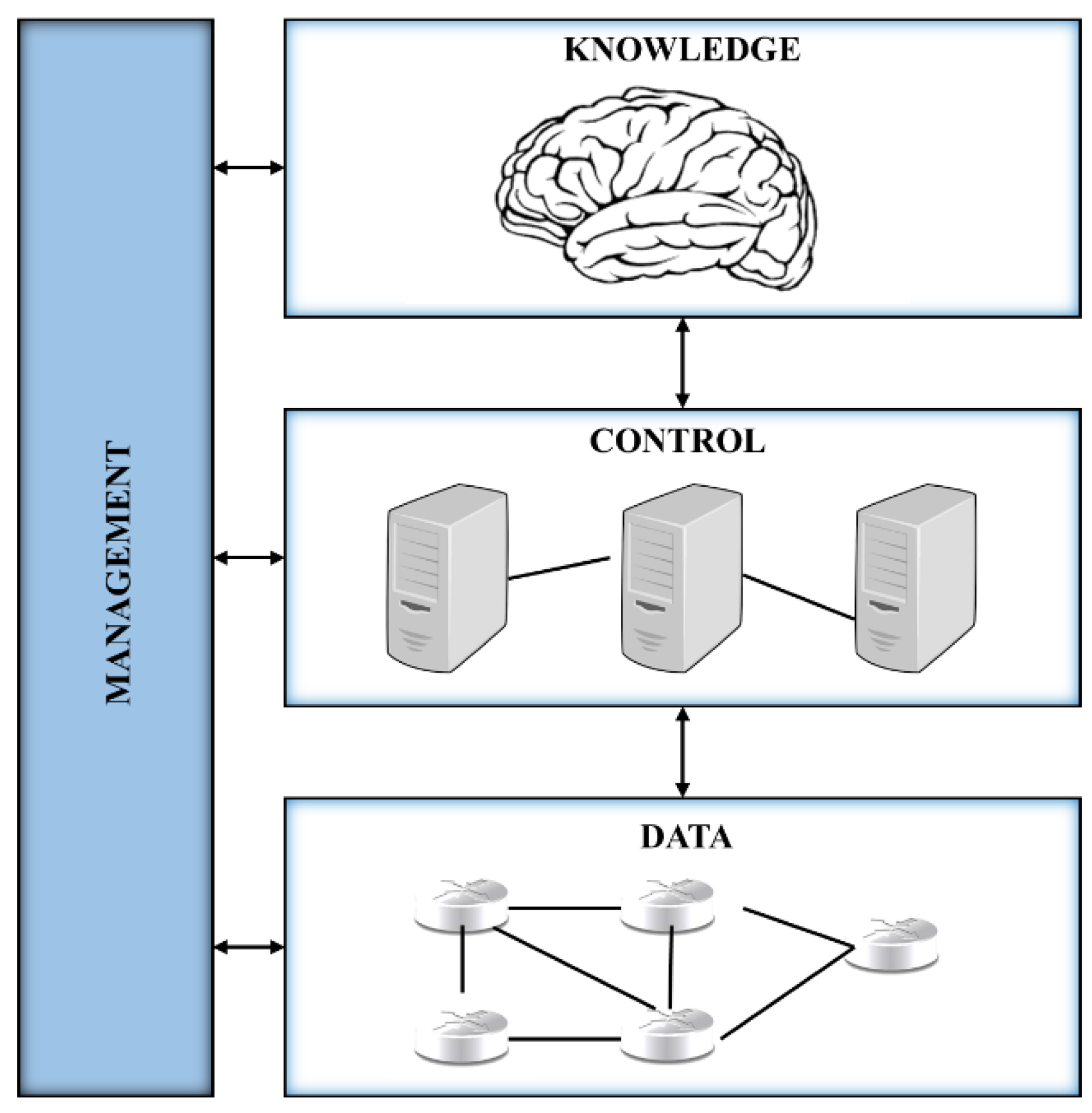
1.1. SDN Model

The Data Plane forwards the data packets. In SDN, the data plane is composed of network devices that can be easily programmed for forwarding via south-bound Application Programming Interface (API) from the controller.

The Control Plane is responsible for the exchange of operational states that enables the data plane to update via south-bound API accordingly. In the SDN setup, it is performed by the centralized controller.

The Management Plane monitors the reliable operation of the network. It helps in configuring data plane elements and outlines the network topology. In the SDN setup, this task is also controlled by the logical centralized controller. The data provided by NA come from the management plane.

To take control over the network the knowledge plane obtains knowledge from the control and network layer. When the KP learns the behavior of the network it can automatically operate the network. Basically, the knowledge plane processes network analytics provided by the management plane, using machine learning to transform it into knowledge; furthermore, this knowledge is used to make decisions [3,5]. Figure 1 illustrates the SDN-with-Knowledge plane.

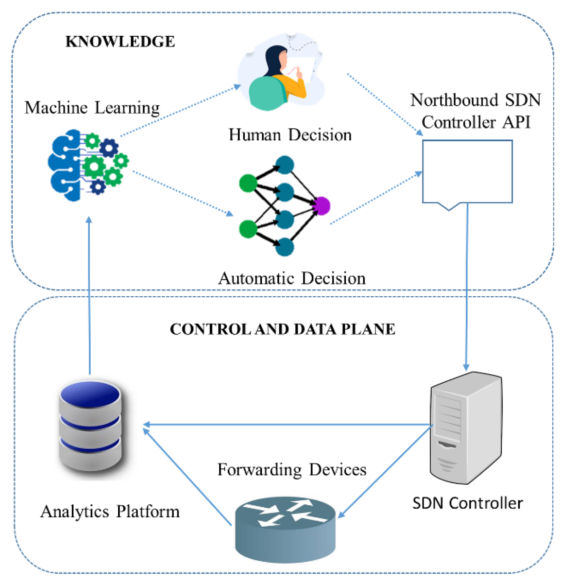
1.2. SDN-with-Knowledge Operation

SDN-with-knowledge borrows some of its ideas from other research areas [1,2,5]. It operates in a control loop, which in turn provides recommendation, optimization, and estimation. A similar approach is also highlighted by other research areas such as neural networks in feedback control systems and automatic network management [14,15]. In addition, the feasibility of our approach is supported by paper [16]. The basic operation of SDN-with-Knowledge is shown in Figure 2, and all entities and their functions are described as follow.

The Analytics Platform is responsible for the collection of information form the network data plane elements such as forwarding devices, switches and routers, and the SDN controller.

Machine learning algorithms play a vital role in KP as they learn the behavior of the network. The information collected by the analytics platform is used by the ML to generate knowledge. Furthermore, ML aids the north-bound controller API to give instructions to the SDN controller on how to operate the network. In the SDN-with-knowledge paradigm, this process is partially assigned to the knowledge plane, which takes advantage of machine learning, makes decisions, and offers recommendations [5].

The SDN controller is responsible for giving control instructions to the forwarding devices via the south-bound protocol, based on the knowledge learned at the KP [5].

1.3. Research Objectives

The objective of this work is to focus on one particular application of the SDN-with-knowledge paradigm and the benefits a knowledge plane combined with machine learning may bring to common networking problems (i.e., resource management in network function virtualization).

1.4. Resource Management in Network Function Virtualization

Here, a use-case is presented which can utilize the concept of the SDN-with-knowledge paradigm in a network setting called network function virtualization [12]. It is a relatively new approach in which network applications, such as firewalls and load balancers, are implemented virtually, called as virtual network functions, without the use of extra hardware [10]; in fact, they are implemented utilizing general hardware.

The management of resources in NFV is very difficult and one of the most researched topics because of its vast applications in Data Centers [12]. The SDN-with-knowledge paradigm has the potential to address resource management problems in NFV [7]. KP with the aid of machine learning techniques can be considered as a new pillar in modeling the resource requirement of VNFs, hence improving the overall performance of the system.

1.5. Machine Learning

ML techniques can be categorized on the basis of the output they produce: Classification and Regression models; furthermore, they can be divided on the basis of the input data they use: Supervised or Unsupervised techniques [6,17].

In classification, the model tries to classify the input in different classes or categories. So, the output value is usually 0 or 1 representing a particular class. On the other hand, the regression models try to learn the continues function for the given input [17]. Similarly, we can say that the regression-based ML model tries to map multiple output continuos functions for the given input. Supervised learning uses labeled input and output data, whereas an unsupervised learning algorithm does not require labeled data. A labeled datum has tags in data fields, such as name, serial number, type, etc., whereas unlabeled data do not contain any tags.

2. Problem Definition and Proposed Models

The considered problem is to check the feasibility of machine learning for accurately estimating the CPU consumption of different virtual network functions deployed in SDN environment, when trained with only traffic features as an input. The CPU needs of a particular VNF depending upon many known and unknown interacting parameters, which is the key motivation factor of using ML-based techniques. Once the ML model is trained, then the CPU’s estimated value can be used by resource allocation schemes [10], which can dynamically assign the required resources to a particular VNF. To solve this resource requirement problem, we preset supervised ML models, Multiple linear regression (MLR), and Support Vector Machine (SVM) in comparison with Artificial Neural Network (ANN). All of the said models are implemented to solve an estimation problem, so they will be termed as multiple linear regression, support vector regression, and fitting neural network, respectively. Furthermore, they are evaluated against each other considering which model best fits the data represented by features.

The main idea is to use a dataset for training our ML models, which can then estimate CPU value for each incoming traffic. For this purpose, first, the dataset must be constructed. Since our proposed models are based on supervised learning, therefore, the dataset must contain a pair of inputs (traffic vector) and outputs (real CPU utilization). The traffic vectors in dataset describes the incoming traffic to the VNFs, while the CPU utilization is the real-world CPU usage of these VNFs when the traffic is processed by them. The traffic is represented by 86 features (number of packets, IP address, total bytes, source and destination address, ports, etc., are a few mentions among others), which are extracted offline in 20 s batches (detail setup in Section 3). Once the dataset is constructed, it is further used to train our proposed ML models, which aim to learn the function that can accurately map the traffic features to CPU consumption. 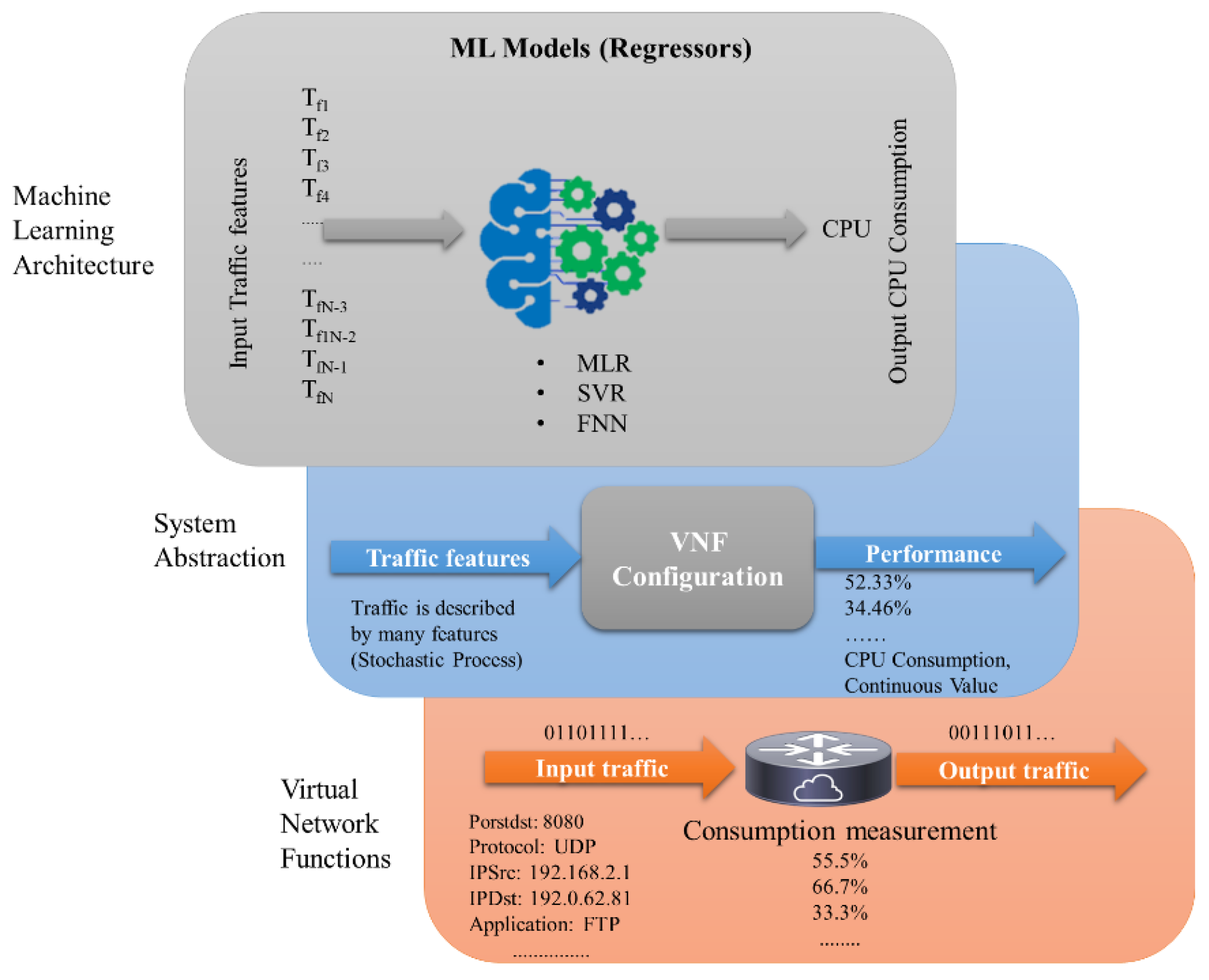Figure 3 defines the considered problem in three layers.

In this work, we modeled the behavior of real-world virtual network function that is shown on the bottom layer in Figure 3. It has been observed that the behavior of a particular VNF depends on different parameters, particularly its configuration, which, in our study, is considered to be constant. In system abstraction, which is the middle layer, the VNF is considered as block box, where the traffic represented by features enters the box and leaves the box, which in turn alters the VNF’s resource requirements. The top layer represents machine learning architecture, where different regressors such as MLR, SVR, and FNN are used to estimate the CPU consumption of VNF. The considered ML models are only trained for CPU estimates of VNF because the exact configuration of VNF is hidden. The following section details the proposed models.

2.1. Multiple Linear Regression

Multiple linear regression analysis is one of the most powerful tools used to model the association between problem variables (i.e., input and output). Modeling the association between these variables can predict future trends [17]. Furthermore, it is used to model the complex relation between dependent variable and multiple independent variables. Assuming $y$ is the dependent variable and $x_1,x_2,x_3\dots \dots \dots ,x_j$ are independent variables, then the MLR regression model can be expressed as follows:

$$y=a_0+a_1{x}_1+a_2{x}_2+a_3{x}_3\dots \dots \dots a_k{x}_k+e,$$

(1)

where $a_0$ is a constant, and $a_1,a_2,\dots \dots ,a_k$ represent regression coefficients.

The main aim of MLR is to minimize the sum of squares of error $\left(\sum e\right)$ by using the Least Square (LS) method [17]. It has been observed that with a large number of dataset observations, this technique gives more robust solutions, but if we have a small number of observations in the dataset, then we obtain poor results.

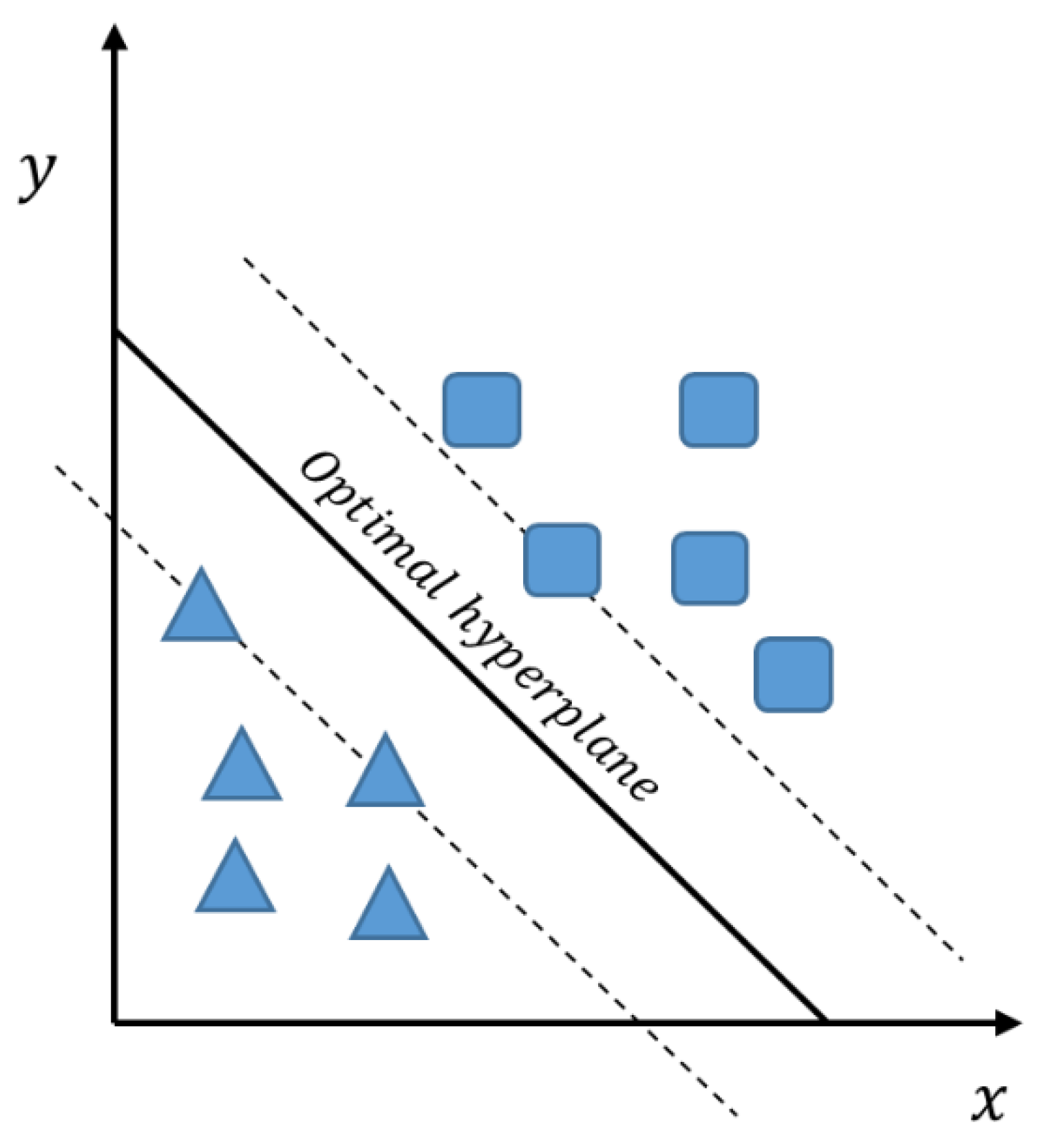
2.2. Support Vector Machines

SVM is a supervised machine learning model widely used for solving regression and classification problems. It was introduced by Vladimir Vapnik et al. at AT&T and Bell Laboratories [18]. SVM maps the training data into higher dimensional space with the help of a nonlinear mapping function also called the kernel function and then applies linear regression to separate data in high-dimensional space [19]. Data Separation is achieved by finding optimum hyperplanes, also called support vectors, that have maximum margins from the separated classes, as shown in Figure 4.

The version of SVM used to solve the estimation problem is called SVR, which is an excellent choice and an efficient method as demonstrated by other related research [19]. Equations (2)–(12) show the principle workings of SVR from a mathematical perspective.

While modelling, the objective of SVM is to find a linear decision function as shown in Equation (2):

$$f\left(x\right)\le \omega ,{\varphi }_i\left(x\right)>+b.$$

(2)

Here, $\omega$ represents the weight vector and $b$ is a constant that has to be estimated from the considered dataset, whereas $\varphi$ is a kernel function or nonlinear mapping function. For the regression problem, the following risk function needs to be minimized:

$$R\left(C\right)=\frac{C}{n}{\displaystyle \sum }_{i=1}^N{L}_{\epsilon }\left(f\left(x_i\right),y_i\right)+\frac{1}{2}\parallel \omega {\parallel }^2,$$

(3)

where $L_{\epsilon }\left(f\left(x_i\right),y_i\right)$ is the $\epsilon -intensivelossfunction$, which is given by the following equation:

$$L_{\epsilon }\left(f\left(x_i\right),y_i\right)=\left\{\begin{array}{cc}\left|f\left(x\right)-y\right|-\epsilon & \left|f\left(x\right)\right|\ge \epsilon \\ 0& otherwise\end{array}\right.$$

(4)

For the attainment of acceptable degree of error, slack variables ${\xi }_{i }$and ${\xi }_i^{*}$ are used, which makes it a constrained minimum optimization problem, as shown in Equation (5):

$$Min.R\left(\omega ,{\xi }_i^2\right)=\frac{1}{2}\parallel \omega {\parallel }^2+ C{\displaystyle \sum }_{i=1}^N\left({\xi }_i+{\xi }_i^{*}\right)$$

(5)

subject to:

$$\left\{\begin{array}{c}{y}_i-<\omega ,x_i>-b\le \epsilon +{\xi }_i\\ <\omega ,x_i>+b-y_i\le \epsilon +{\xi }_i^{*}\\ {\xi }_i,{\xi }_i^{*}\ge 0\end{array}\right.$$

(6)

where$C$ is a regularized constant, which is greater than zero, and provides equilibrium between training error and flatness of model. $C$ is also a penalty for the estimation of error (i.e., greater than $\epsilon$). ${\xi }_{i }$and ${\xi }_i^{*}$ are slack variables that represent the distance of actual values to corresponding boundary values of $\epsilon$. SVM tries to minimize ${\xi }_{i }, {\xi }_i^{*} ,$and ${\omega }^2$. A quadratic programming problem can be achieved by converting the above optimization with constraint to Lagrangian multipliers as follows:

$$f\left(x\right)={\displaystyle \sum }_{i=1}^N\left({\alpha }_i-{\alpha }_i^{*}\right)K\left(x_i,x\right)+b$$

(7)

where $\left({\alpha }_i\right.$ and $\left.{\alpha }_i^{*}\right)$are Lagrange multipliers. Equation (7) is subject to following conditions:

$${\displaystyle \sum }_{i=1}^N\left({\alpha }_i-{\alpha }_i^{*}\right)=0$$

(8)

where $0\le {\alpha }_i\le C, i=1,\dots ,n$ and $0\le {\alpha }_i^{*}\le C, i=1,\dots ,n.$ Here, $K$ represents the kernel function, and its value can be obtained from the inner product of $x_i$and $x_j$ in feature spaces $\varphi \left(x_i\right)$ and $\varphi \left(x_j\right),$ respectively, which satisfies Mercer’s rule. Therefore:

$$K\left(x_i,x_j\right)=\varphi \left(x_i\right).\varphi \left(x_j\right)$$

(9)

In general, SVM has an advantage over MLR and ANN in high-dimensional space, especially when then the size of training data set is small because the support vectors rely only on a small subset of training data, hence giving a computational advantage to SVM over other classical techniques.

2.3. Artificial Neural Networks

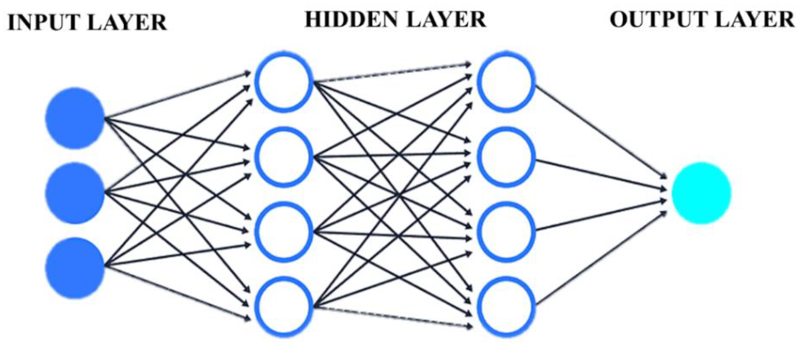
ANNs are ML tools which work on the concept of biological neurons and their inter-connections. ANNs are composed of multiple units in which each unit is called a neuron that takes multiple input signals and converts it to a single output signal with the help of the activation function [20,21]. Therefore, it can be used to solve classification, pattern recognition, and estimation problems [20,21,22]. Interconnections of neurons form a network; in fact, they form a layered structured network, in which the first one is the input layer, the last one is the output layer, and in-between any number of layers are called hidden layers [20,22], as shown in Figure 5.

The mathematical function which is repeatedly performed inside ANN is given by Equation (10):

$$\mathrm{Y}=\mathsf{\sigma }\left[{{\displaystyle \sum }}_{i=1}^n\left(w_{ij}{a}_i+b_i\right)\right]$$

(10)

where $\mathsf{\sigma }$ denotes the activation function applied to the weighted sum of all inputs from this layer, whereas $W_{i.j}$ is corresponding weights of this layer. $a_i$ is the input of this layer, and $b_i$ is the bias of this layer. During the “learning” phase, the aim is to find the optimal value of $W_{i.j}$ and $b_i$ parameters for each layer, which is attained by minimizing the cost function called the mean squared error (MSE) as follows:

$$MSE=\frac{1}{n}{\displaystyle \sum }_{i=1}^N{\left(y_i-{\widehat{y}}_i\right)}^2$$

(11)

where $y$ represents the actual output (target), and $\widehat{y}$ is the estimated or predicted value by ANN.

The performance of ANN depends on combination of multiple parameters such as the learning rate, number of neurons, hidden layers, optimization algorithm, and activation function [20]. In this work, ANN is implemented using the same configuration provided by paper [7], so the results from this model can be compared with our proposed regression models, namely, MLR and SVR. The ANN in [7] has three layers: the input, the output layer, and only one hidden layer in-between. Furthermore, the backpropagation algorithm is used for optimization. The activation function used in this work is sigmoid, which is given by Equation (12):

$$\varphi \left(S\right)=\frac{1}{1+e^{-S}}$$

(12)

2.4. Evaluation Criterion

In order to assess the performance and accuracy of proposed models, two evaluation criteria are used to measure how close the predicted value by these models are to the real value (target value). Firstly, the “regression accuracy” of these models are calculated by means of correlation coefficient $R$ given by Equation (13). $R$ is a correlation coefficient, between the actual outputs and the predictions of each model. A correlation coefficient of $R=1$ shows $100\%$ prediction accuracy, i.e., prediction equals target value:

$$R=\frac{{\sum }_{i=1}^n \left(y_i-\overline{y}\right)\left({\widehat{y}}_i-\overline{\widehat{y}}\right) }{\sqrt{{\sum }_{i=1}^n{\left(y_i-\overline{y}\right)}^2{\sum }_{i=1}^n{\left({\widehat{y}}_i-\overline{\widehat{y}}\right)}^2 }}$$

(13)

where $y$ is the actual output or desired output, $\widehat{y}$ is the value estimated by our ML models, and $n$ represents the total number of observations.

Furthermore, the accuracy of the predictions for the three ML models in terms of cumulative distribution function (CDF) of “percentage prediction error” is used. Accuracy results in the form of CDFs of error are perhaps more useful from a design and analysis perspective. Typically, the prediction performance of the ML tools is interpreted with a target or admissible prediction error

3. Methodology

To assess the performance of our proposed solution, the whole experimental setup provided by [7] was reproduced using a real traffic trace. The purpose was to further validate the data set already publicly available [23]. The traffic represented by features, was processed by different VNFs, and the averaged CPU consumption was monitored in 20 s batches [7]. A set of network, transport, and application layer attributes (total 86 features) were used to describe the traffic. The data set was made by using these traffic features as an input, while the average central processing unit was used as an output.

Once the data set was generated, it was further used to train supervised ML models (i.e., MLR, SVR, and FNN). Then, the accuracy of these frameworks were evaluated using the cross-validation technique. The data set was further split into two sets: the training set contained 70% of the total samples, while the remaining 30% of the samples were assigned to the test set.

The training set as used to train the ML model during the training phase, while the test set was used to further validate the model. Finally, the CPU consumption estimated by the ML technique was compared with the actual measurements.

3.1. Virtual Network Functions VNFs

The experiment was performed by deploying Virtual Machines (VMs), which implements two different VNFs: Open virtual switch (OVS) [24,25] and Snort [25,26]. OVS is an open source implementation of SDN multilayer switch, while Snort is a network anomaly detection and prevention system, which can analyze the traffic.

In this work, OVS was implemented using two different configurations. The first implementation used the default settings, which forwards most of the packets and sometimes forward the packets to the SDN controller when necessary, so the controller can inspect the packets and install new forwarding rules in the OVS, which expires every 20 s. The second implementation does not forward the packets to the controller, and OVS acts as a firewall by implementing more than 300 rules. For Snort VNF, only a single configuration was used, which is the default setting and detects most of the anomalies in the network.

3.2. Traffic Preprocessing

Preprocessing of the data was usually carried out to make the data compatible with the desired ML models. The raw data were synthesized and converted to a form which could be easily utilized by our proposed ML models. The real traffic trace is used to test the performance of different VNFs. From the on-campus interconnection link, which was 10 Gbps (both incoming and outgoing), 2 traffic traces, each 5 min long, were captured at two different moments. These traffic traces were then used to reproduce the traffic in experimental environment, which was further sent to virtual network functions, and the respective CPU consumption was monitored.

For synthesis of the data in the test environment, the speed of the link as considered too high. Therefore, we scaled it by dividing the rate by 10 for day time and 40 for the night time, which resulted in approximately 2000 packets/s. The traffic was described by a set of 86 features from the network to transport layers.

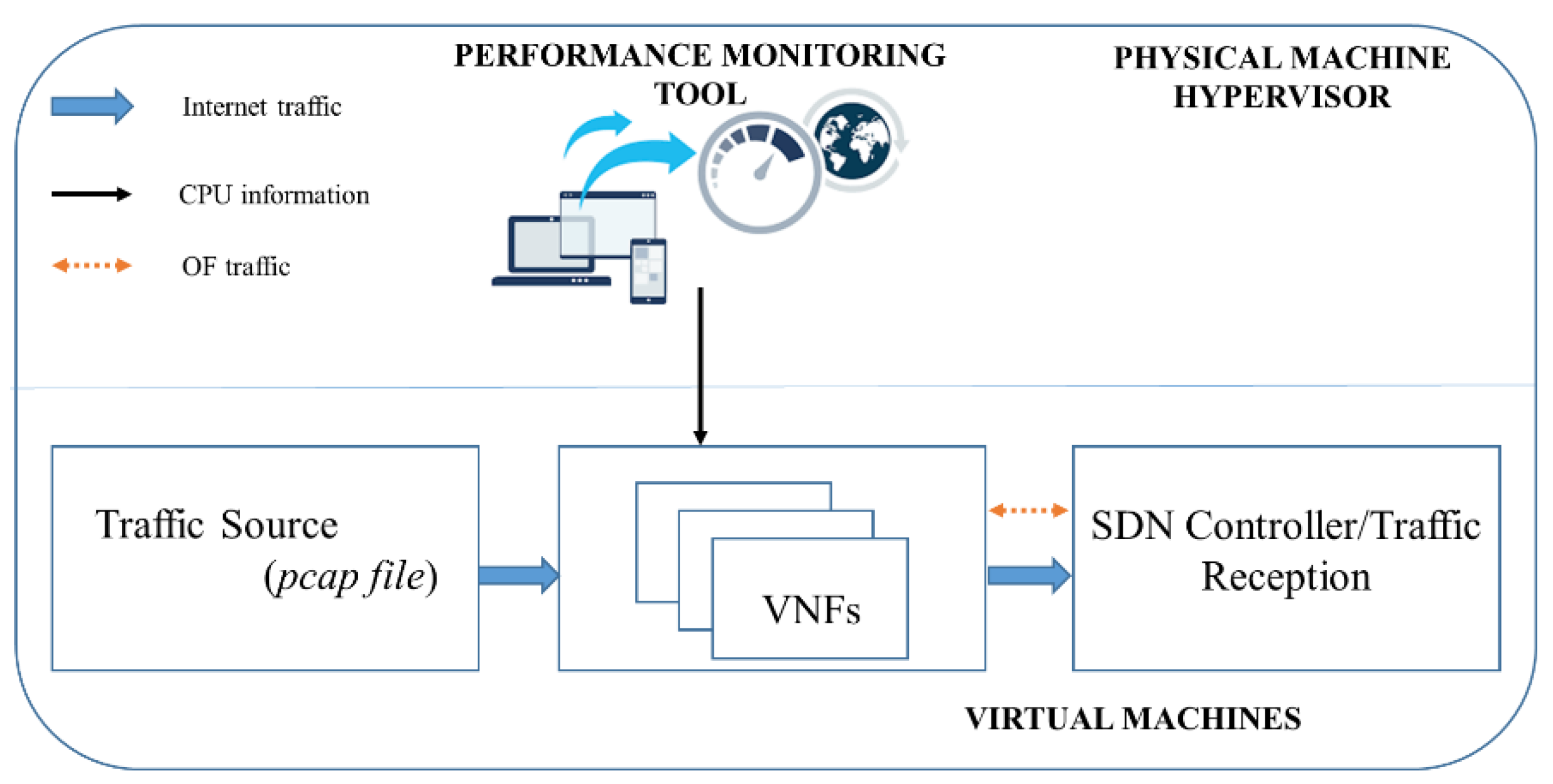
Components needed for the completion of our experiments were deployed in the single physical machine monitored by hypervisor. All the virtual machines (VMware ESXi v5.5) deployed under the hypervisor were connected with virtual links (gigabit). Traffic was generated from one virtual machine and sent to another VM where the VNF was installed. TCPreplay (v 3.4.4) was used to replay the traffic. Each VNF (Firewall, OVS, Snort) was installed on separate virtual machines, and CPU consumption was monitored with the performance monitoring tool of the hypervisor. Another VM was installed as SDN controller, which receives the traffic from VNF working as OVS, when necessary. Figure 6 shows the complete configuration setup.

The hypervisor performance monitoring tool (Virtualization manager v2020.2.1) was used to manage and analyze the VMs performance under a single umbrella. Virtualization manger is a very powerful tool developed by SolarWinds which can monitor the CPU, memory, and storage needs in real time with good accuracy [27]. Out of various output parameters available, only the CPU load was used because the results need to be compared and analyzed with the state-of-the-art, which uses the same parameter. This will help us to adopt the best ML model in the current scenario.

The data set was generated by collecting traffic features as an input while the average central processing unit utilization as the output. A total of 755 data points were collected for firewall, 1172 for OVS, and 1359 for Snort VNF. Our collected data set showed exactly the same behavior when applied to ML models, with the one that is publicly available at [23], which further validates the data set, but for fair comparison with the state-of-the-art, we used the same data set publicly available at [23].

3.3. Machine Learning Training

In this work, we have selected MLR and SVR, which are compared and analyzed against state-of-the-art FNN to identify the best estimator which can accurately predict CPU load for VNF. To train MLR and SVR, we have used MATLAB Statistics and Machine Learning Toolbox 11.5 while Deep Learning toolbox 12.1 is used to train the FNN. The traditional technique MLR model requires little to no parameter tweaking, which means the default settings of the toolbox, with preset and term parameters set to linear and robust parameters set to off, were used. Furthermore, the mathematical function performed by MLR technique on the data set was be based on Equation (14), which can be written as following.

$$y=a_0+{{\displaystyle \sum }}_{i=1}^{86}{a}_i{x}_i$$

(14)

The LS estimation function was used to estimate the values of parameter $a^{\prime }s$, which gave us optimal values for parameters ${\widehat{a}}^{’}s$.

For developing the SVM model, the main aim was to minimize the $\epsilon -intensivelossfunction$ on the training data set, which can be achieved by selecting the appropriate kernel function. For this purpose, all the well-known kernel functions (Linear, quadratic, Gaussian, and cubic) in the MATLAB Statistics and Machine Learning Toolbox were first tested, and finally, SVM with polynomial cubic kernel was used to develop our model, since it outperformed all the other models for our considered data set. Furthermore, parameters such as kernel scale, box constraint, and Epsilon are set to automatic, which is the default setting. Cubic kernel has many advantages over other kernel functions, such as it can easily map non-linearity in the training data.

The FNN was implemented using the same configuration provided by paper [7], which had three layers. The input layer consisted of 86 inputs neurons, while the output layer had only 1 output neuron, in-between only 1 hidden layer with 5 neurons. We also tested the FNN with different numbers of neurons, but empirically, we have learned that the best number of neurons in the hidden layers is five because this number provided the minimum value of MSE in the training and testing phase. In addition, different activation functions were tested in the hidden layer, and sigmoid was selected, which gave the best results among others. Further increasing the number of neurons in the hidden layer gave rise to the overfitting problem in FNN. The Levenberg–Marquardt algorithm was used for the weight optimization of FNN. The next section details the overall system performance of MLR, SVR, and FNN in terms of regression accuracy and percentage error.

4. Experimental Results

This section details the experimental results and their explanation. First, prediction results for each VNF via different ML techniques are presented.

4.1. Accuracy in Terms of Regression

Figure 7, Figure 8 and Figure 9 show the regression plots for the firewall, OVS, and Snort VNFs, respectively, in the three ML models considered in this work. On the x-axis, we have a target which is the desired output, i.e., the real CPU consumption calculated through experiment. On the y-axis, we have the predicted output calculated by the ML models. The figure also provides the correlation factor $R$, according to Equation (13), as described in Section 2.4, between the actual outputs and the predictions of each model. A correlation factor of $R=1$ shows $100\%$ prediction accuracy, in which case the linear fit (solid line) of the ML model becomes aligned with diagonal (dotted line) labelled Y = T, i.e., prediction equals target value.

For the firewall VNF in Figure 7, the most accurate predictions are delivered by the SVR technique. This is evident from the correlation factor approaching 1 and the linear fit almost aligned with diagonal best fit. Predictions from the MLR model are slightly worse with $R=0.97259$. Surprisingly, predictions from the FNN are the least accurate among the considered models, although FNN is a more sophisticated tool. One possible reason for the low accuracy of FNN predictions might be the data set size of the firewall VNF. The set of 755 data points for the firewall function might be too small for the single-layer FNN. Improvement in the prediction accuracy of the FNN in the following VNFs with larger data set sizes provides support to this conjecture.

Figure 8 shows the regression plots for the Open vSwitch VNF. The SVR model produces the most accurate predictions with correlation factor $R=0.99629$, while the FNN produces the least accurate predictions. In terms of the correlation factor, the predictions of the SVR are equally accurate as in the case of firewall VNF. OVS predictions of the MLR model exhibit a degradation compared to those of the firewall. The accuracy of the OVS predictions from FNN show a considerable improvement with respect to the firewall case.

Finally, Figure 9 presents the regression plots for the Snort VNF. Here, again, the SVR produces the most accurate predictions followed, in decreasing order of accuracy, by MLR and FNN. It is interesting to note that the accuracy of the FNN predictions improves significantly for OVS and Snort functions with larger data sets of 1172 and 1359 data points, respectively. The prediction accuracy of the SVR model remains practically the same for the three VNFs. On the other hand, prediction accuracy of the MLR degrades slightly for the OVS and Snort network functions. Figure 7, Figure 8 and Figure 9 demonstrate that the SVR produces the most accurate predictions for the considered VNFs. The correlation factors $R$ of all the results from Figure 7, Figure 8 and Figure 9 are shown in

Table 1. The correlation factor $R$ of all the results from Figure 7, Figure 8 and Figure 9.

Framework	$\mathbf{Firewall}\mathbf{Coefficient}\mathit{R}$	$\mathbf{OVS}\mathbf{Coefficient}\mathit{R}$	$\mathbf{Snort}\mathbf{Coefficient}\mathit{R}$
MLR	0.97259	0.94898	0.94991
SVR	0.99697	0.99629	0.99577
FNN	0.80096	0.92623	0.92819

.

4.2. Accuracy in Terms of Error Percentage

Figure 10, Figure 11 and Figure 12 present the accuracy of the predictions for the three ML models in terms of CDFs of percentage prediction error.

First, Figure 10 shows prediction accuracy of MLR for the three VNFs. It can be seen in the figure that the percentage error in the predictions of MLR is limited to 8% most of the time. For a desired percentage error of up to 8%, prediction accuracy of MLR is very close to each other for the three VNFs, with the accuracy for firewall being slightly better. This is in agreement with the prediction accuracy indicated by correlation factor in results of Figure 7, Figure 8 and Figure 9. However, the prediction accuracy for the three VNFs is not the same if the desired prediction accuracy is higher. For example, if prediction error of up to 2% is admissible, then MLR predictions are accurate 60% of the time for the OVS function, while those for the Snort function are accurate approximately 45% of the time. Alternatively, if the 80th percentile is observed, MLR predictions for Snort contain up to 4% errors, while those for OVS up to almost 3% errors.

Figure 11 shows the CDFs of percentage errors in predictions for the firewall, OVS, and Snort using the SVR model. It can be seen that prediction errors are limited to 4% in almost all cases and are limited to even 2% with a probability exceeding 0.95. For the 80th percentile, the prediction errors are limited to 1%, with predictions for OVS being marginally more accurate.

Figure 12 shows the CDF of the error percentages in the predictions of the FNN. For all the considered VNFs, errors in the predictions of FNN are visibly large compared to SVR and MLR (cf. Figure 10 and Figure 11, respectively). The FNN is able to produce relative accurate predictions for the OVS function. Predictions for the firewall function are least accurate.

5. Discussion

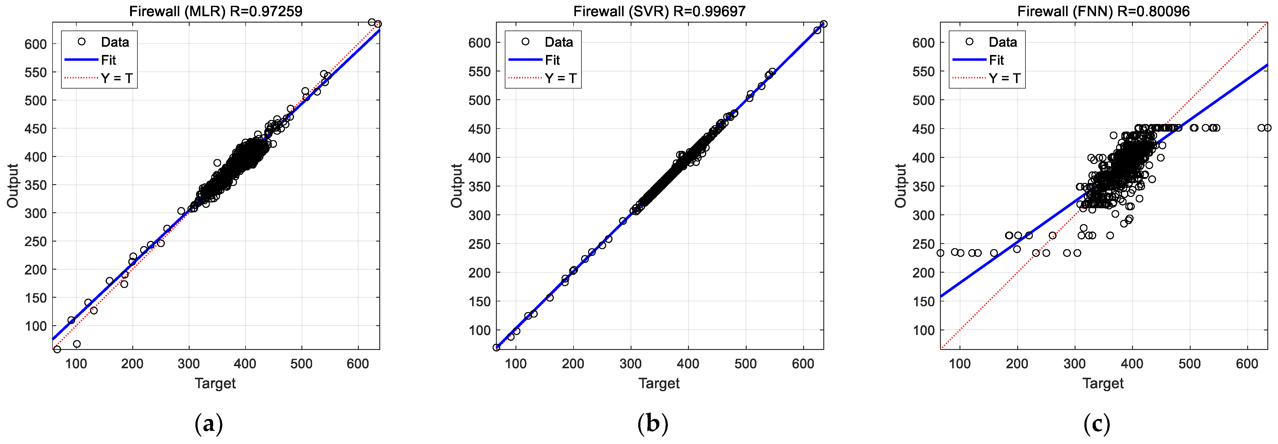
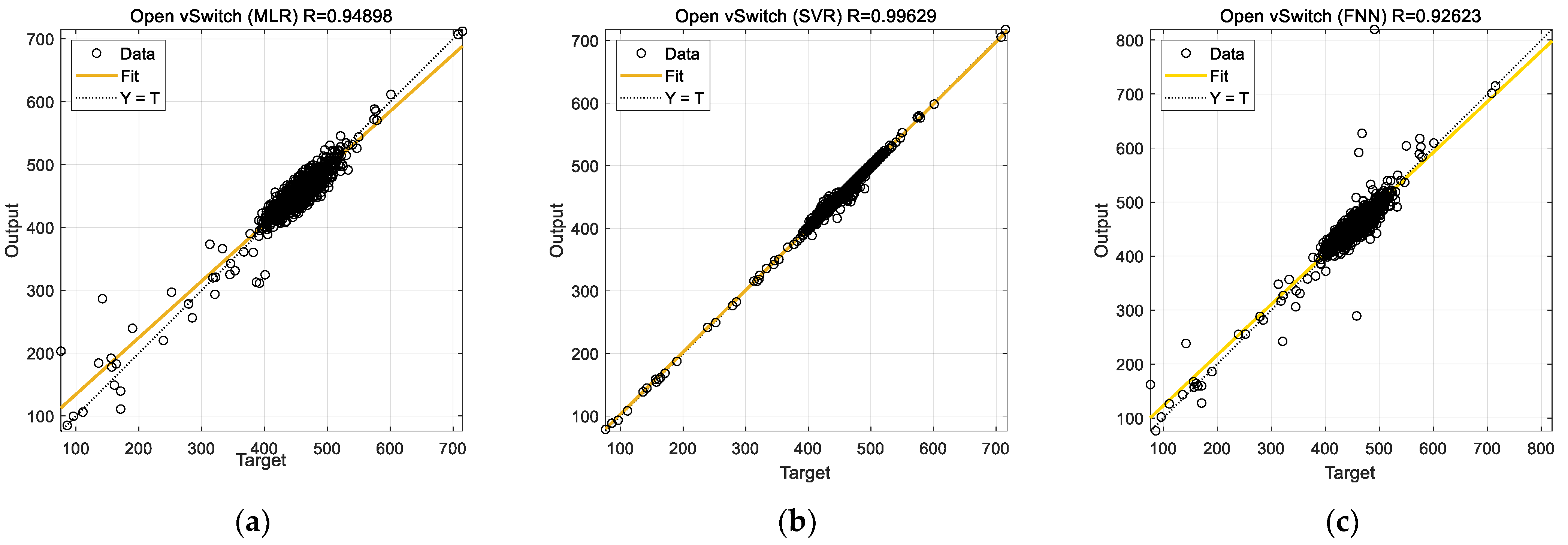
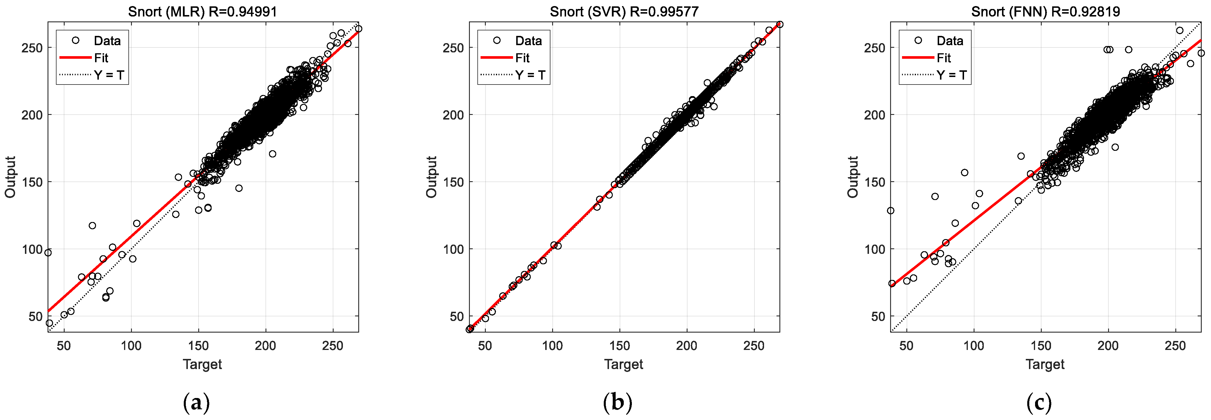
In this section, experimental results from the previous section are discussed. The results concerned prediction of the CPU usage of three VNFs, namely, firewall, OVS, and Snort via different ML models (MLR, SVR, and FNN). The regression plots for predictions (cf. Figure 7, Figure 8 and Figure 9) suggest the superiority of the SVR model in terms of prediction accuracy for the considered VNFs. The prediction accuracy of the FNN for the firewall function is considerably low. Especially, the FNN is very inaccurate in predicting extreme (both low and high) CPU usage (cf. Figure 7c). Although prediction accuracy of FNN improves significantly for the OVS and Snort functions, it remains inferior to MLR and SVR in all the studied cases.

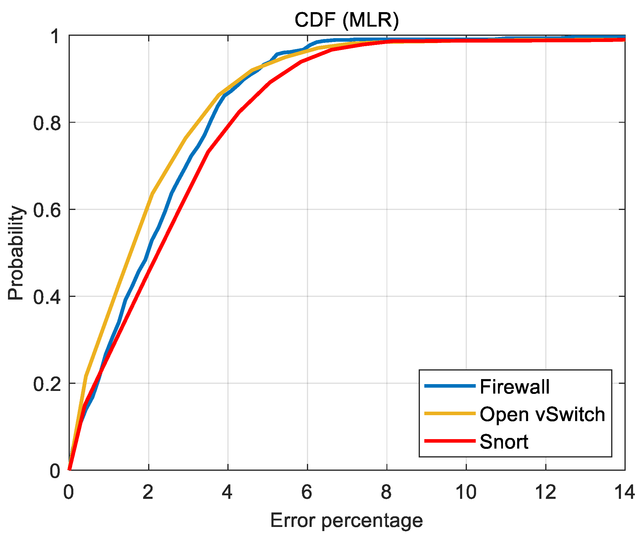
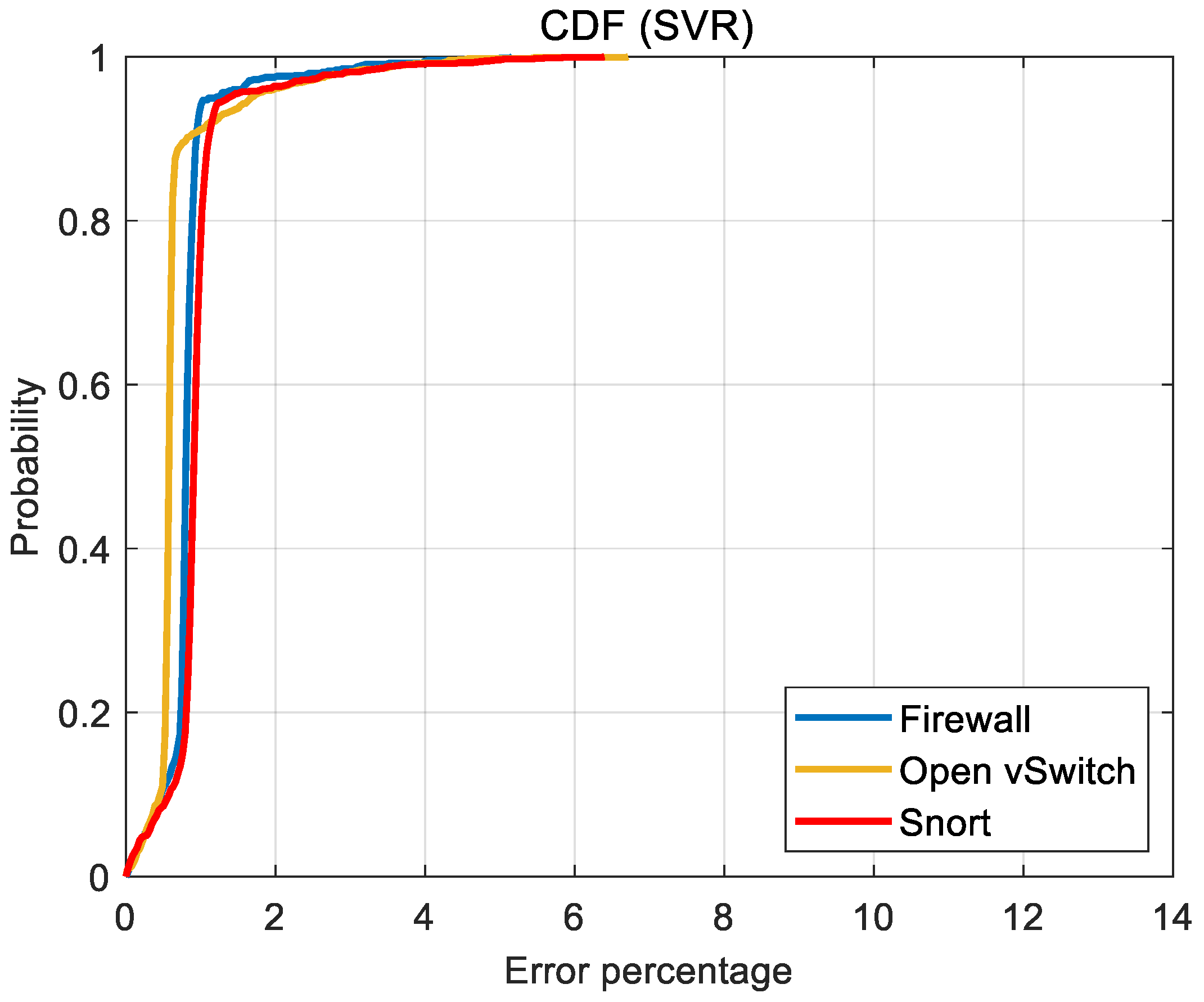
Accuracy results in the form of the CDFs of error (Figure 10, Figure 11 and Figure 12) are perhaps more useful for the design and analysis of SDN. Typically, the prediction performance of the ML tools is interpreted with a target or admissible prediction error. For the following discussion, it is assumed that up to a 2% prediction error is admissible. Then, it is of interest to see how frequent the error in the ML predictions is admissible. For the SVR, the prediction error is admissible at least approximately 95% of the time for all the studied VNFs. On the other hand, both the MLR and FNN produce acceptable predictions only 60% of the time for their best cases, i.e., OVS.

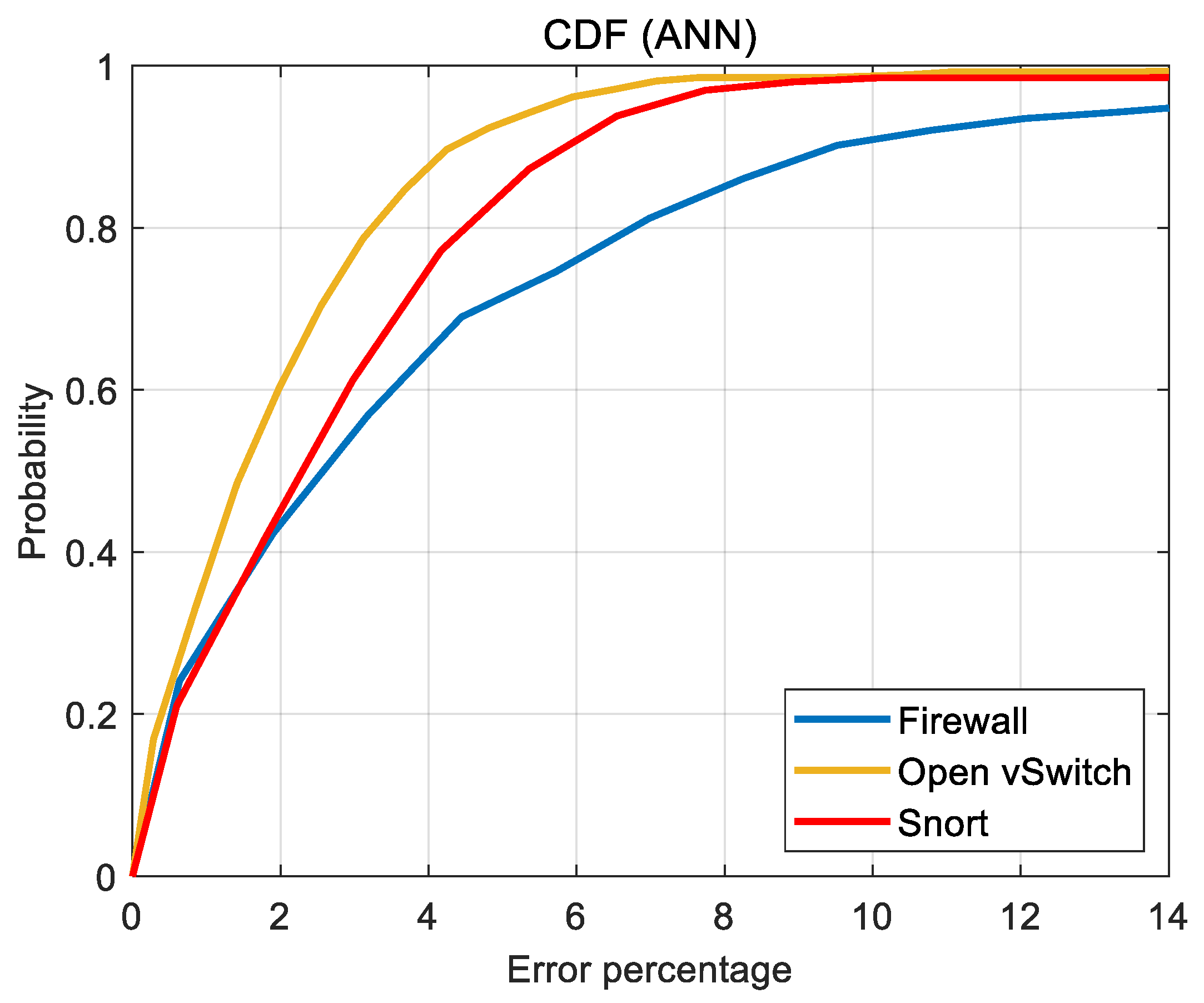
The computational nature or data set size of the VNF appears to have negligible effect on the prediction accuracy of the SVR. On the other hand, prediction accuracy of FNN shows significant variations with data set size. Moreover, for the acceptable error of up to 2%, MLR prediction accuracy improves as the computational intensity of the VNF increases i.e., predictions of OVS are more accurate than those of Snort (cf. Figure 10). However, such a clear trend with respect to computational intensity of the VNF cannot be seen in the FNN predictions (cf. Figure 12).

The poorer prediction performance of FNN, especially in the case of firewall, can be attributed to the relatively small data set size for firewall CPU usage. The prediction performance of FNN can be improved by deploying a deeper ANN with multiple hidden layers. Moreover, the FNN can be complemented with principal component analysis for improving its prediction accuracy. Nevertheless, exploiting the true potential of an ANN typically requires a sufficiently large data set. Therefore, it will be an interesting future work to compare the prediction accuracy of the ML models for a larger and equal-sized data sets for each VNF.

6. Conclusions

In this work, we investigated supervised ML techniques, namely, MLR, SVR, and FNN, to model resource requirements, particularly the CPU consumption of complex network entities such as virtual network functions deployed in software defined networks. A total of 86 input features from the transport to application layer were used to model the association of these input to corresponding output, which is CPU consumption. The feasibility of such an approach is validated by the obtained results and other research work, mentioned in the related work. Our experiments demonstrated that ML techniques can be used to model the resource requirements of different VNF. The results obtained suggest the superiority of the SVR model in terms of prediction accuracy for the considered VNFs over MLR and FNN, which is further validated by CDFs of the percentage prediction error.

Moreover, the prediction performance of FNN can be improved by deploying a deeper ANN with multiple hidden layers. Exploiting the true potential of an ANN typically requires a sufficiently large data set. Therefore, it will be an interesting future work to compare prediction accuracy of the ML models for a larger and equal sized data sets for each VNF. In this study, only the CPU load of different VNFs is modeled using ML techniques; however, in the future, the study can be extended to model and investigate other computer resources such as memory usage, secondary memory usage, or storage requirements.