
Current Sensorless MPPT Control for PV Systems Based on Robust Observer


Abstract
:1. Introduction
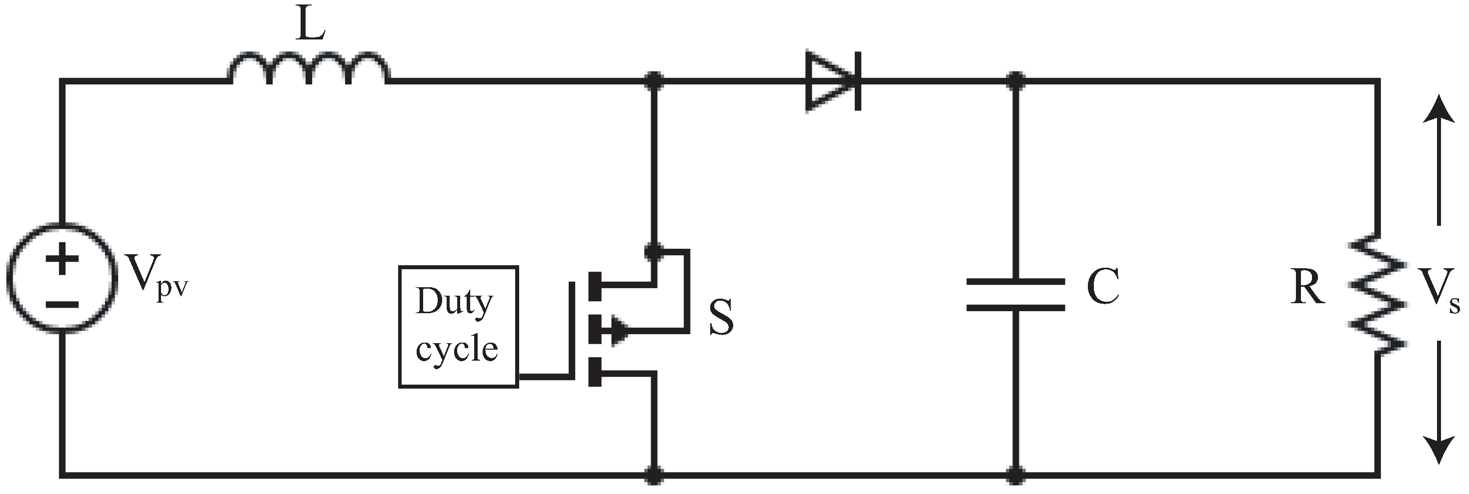
2. System Modeling
Boost Converter Model
3. Problem Formulation
3.1. Mathematical Preliminaries
3.2. Bounded System Model Representation
4. Design of Luenberger Robust Observer Based on AEM
Incremental Conductance MPPT Algorithm
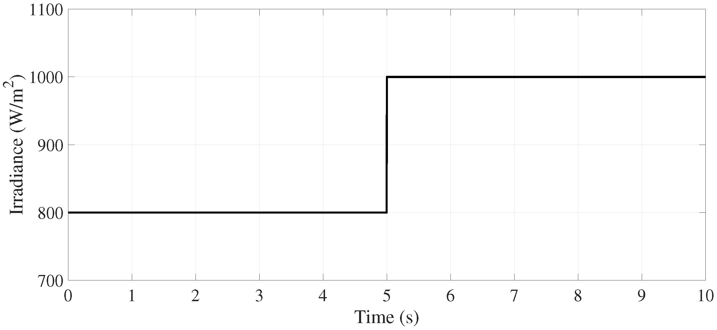
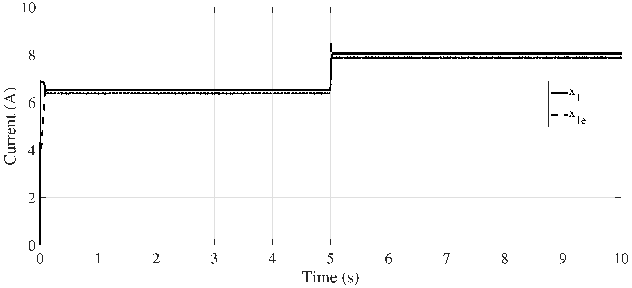
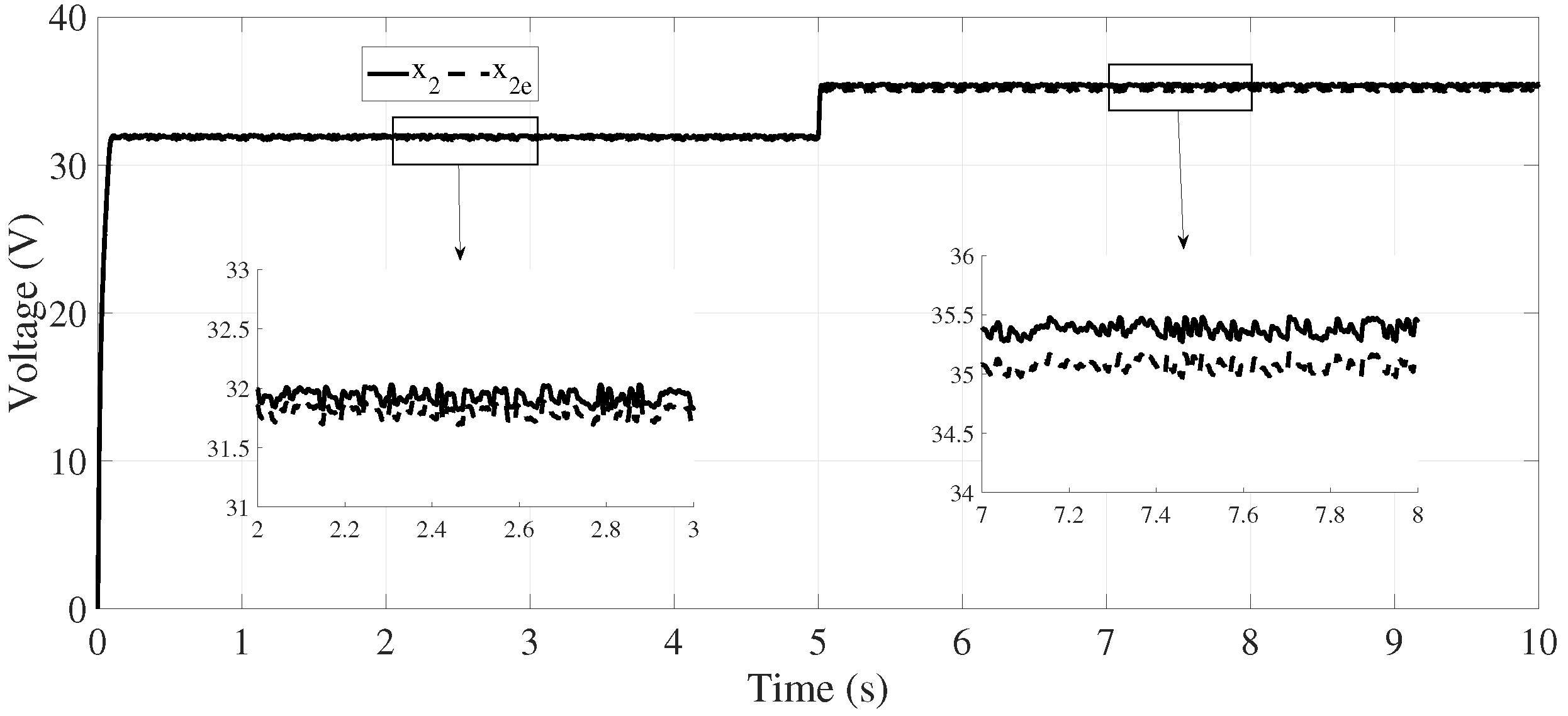
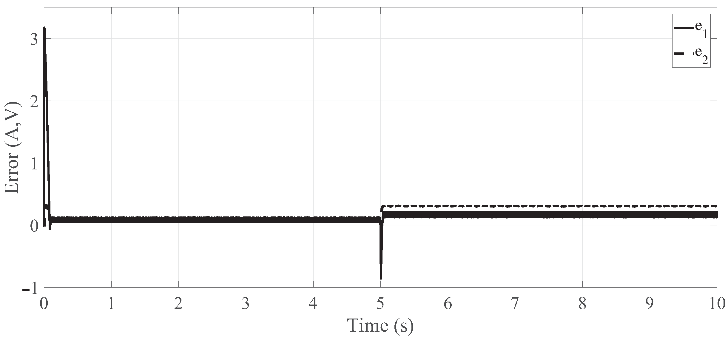
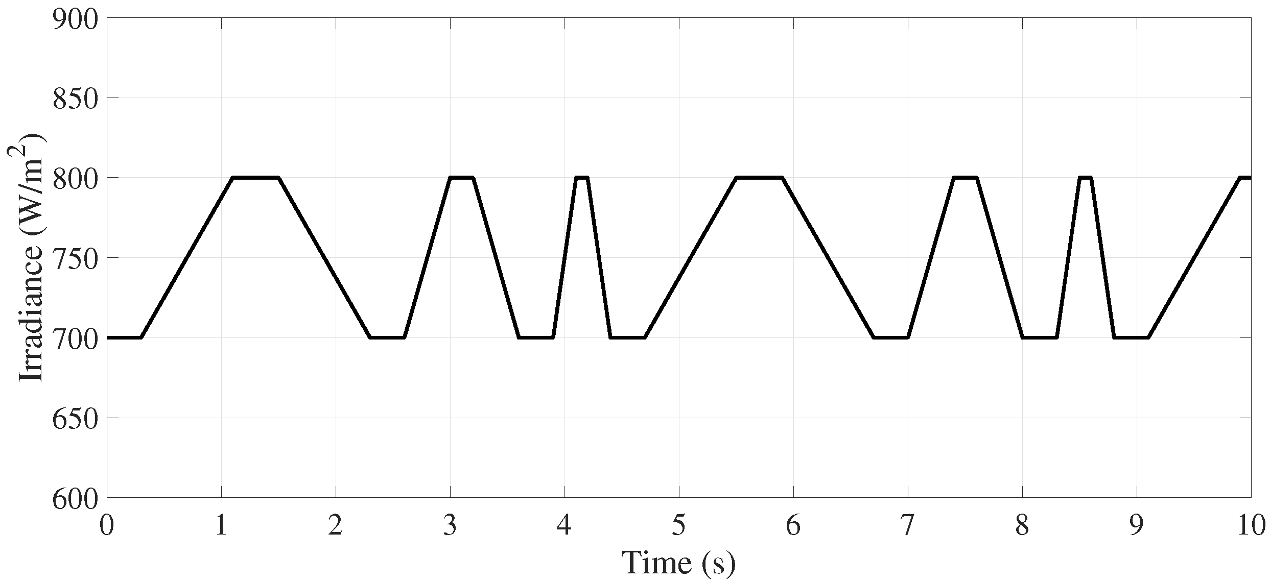
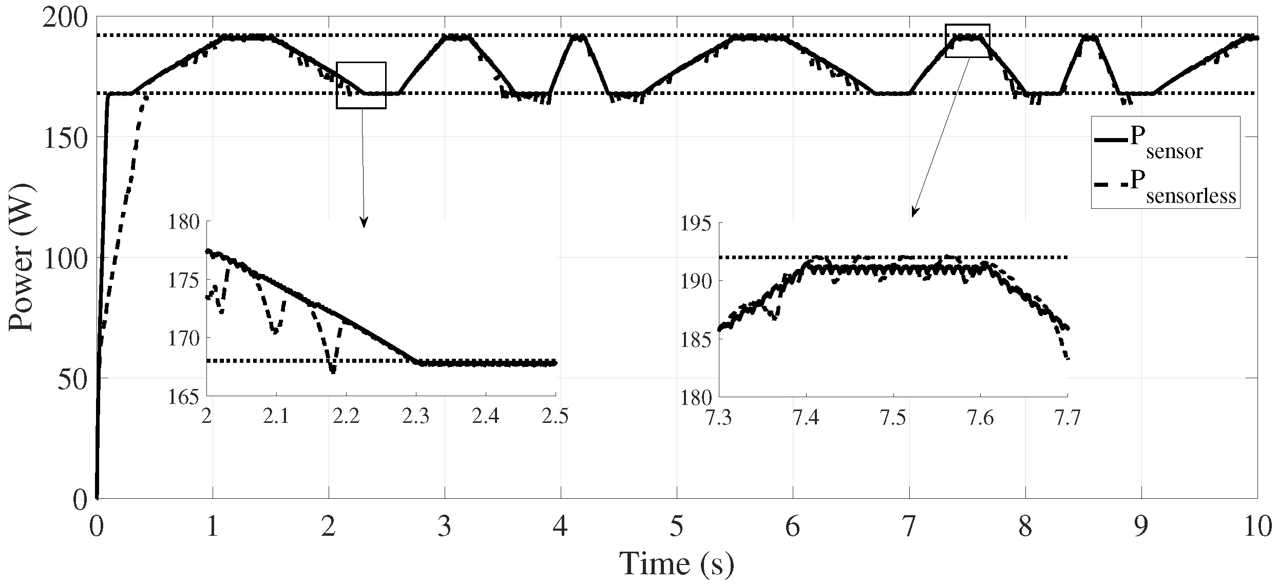
5. Results
6. Conclusions
Author Contributions
Funding
Data Availability Statement
Conflicts of Interest
References
- Kollimalla, S.K.; Mishra, M.K. Variable perturbation size adaptive P&O MPPT algorithm for sudden changes in irradiance. IEEE Trans. Sustain. Energy 2014, 5, 718–728. [Google Scholar]
- Loukriz, A.; Haddadi, M.; Messalti, S. Simulation and experimental design of a new advanced variable step size Incremental Conductance MPPT algorithm for PV systems. ISA Trans. 2016, 62, 30–38. [Google Scholar] [CrossRef] [PubMed]
- Messalti, S.; Harrag, A.; Loukriz, A. A new variable step size neural networks MPPT controller: Review, simulation and hardware implementation. Renew. Sustain. Energy Rev. 2017, 68, 221–233. [Google Scholar] [CrossRef]
- Kulaksız, A.A.; Akkaya, R. A genetic algorithm optimized ANN-based MPPT algorithm for a stand-alone PV system with induction motor drive. Sol. Energy 2012, 86, 2366–2375. [Google Scholar] [CrossRef]
- Algazar, M.M.; El-Halim, H.A.; Salem, M.E.E.K. Maximum power point tracking using fuzzy logic control. Int. J. Electr. Power Energy Syst. 2012, 39, 21–28. [Google Scholar] [CrossRef]
- Life Energy Motion (LEM). Datasheet: Current Transducer LTSR 6-NP. 2017. Available online: www.lem.com (accessed on 7 April 2022).
- Ziegler, S.; Woodward, R.C.; Iu, H.H.C.; Borle, L.J. Current sensing techniques: A review. IEEE Sens. J. 2009, 9, 354–376. [Google Scholar] [CrossRef]
- Chen, Y.; Huang, Q.; Khawaja, A.H. An interference-rejection strategy for measurement of small current under strong interference with magnetic sensor array. IEEE Sens. J. 2018, 19, 692–700. [Google Scholar] [CrossRef]
- Honeywell. Hall Effect Sensing and Application. Available online: https://sensing.honeywell.com/honeywell-sensing-sensors-magnetoresistive-hall-effect-applications-005715-2-en2.pdf (accessed on 15 December 2021).
- Itzke, A.; Weiss, R.; Weigel, R. Influence of the conductor position on a circular array of Hall sensors for current measurement. IEEE Trans. Ind. Electron. 2018, 66, 580–585. [Google Scholar] [CrossRef]
- Min, R.; Tong, Q.; Zhang, Q.; Zou, X.; Yu, K.; Liu, Z. Digital sensorless current mode control based on charge balance principle and dual current error compensation for DC–DC converters in DCM. IEEE Trans. Ind. Electron. 2015, 63, 155–166. [Google Scholar] [CrossRef]
- Yu, B.; Abo-Khalil, A.G. Current estimation based maximum power point tracker of grid connected PV system. In Proceedings of the 2013 IEEE 10th International Conference on Power Electronics and Drive Systems (PEDS), Kitakyushu, Japan, 22–25 April 2013; pp. 948–952. [Google Scholar]
- Wang, Y.; Liu, Y.; Wang, C.; Li, Z.; Sheng, X.; Lee, H.G.; Chang, N.; Yang, H. Storage-less and converter-less photovoltaic energy harvesting with maximum power point tracking for internet of things. IEEE Trans. Comput.-Aided Des. Integr. Circuits Syst. 2015, 35, 173–186. [Google Scholar] [CrossRef]
- Ahmed, M.; Abdelrahem, M.; Kennel, R.; Hackl, C.M. A robust maximum power point tracking based model predictive control and extended Kalman filter for PV systems. In Proceedings of the 2020 International Symposium on Power Electronics, Electrical Drives, Automation and Motion (SPEEDAM), Sorrento, Italy, 24–26 June 2020; pp. 514–519. [Google Scholar]
- Mattavelli, P. Digital control of DC-DC boost converters with inductor current estimation. In Proceedings of the Nineteenth Annual IEEE Applied Power Electronics Conference and Exposition, 2004. APEC’04, Anaheim, CA, USA, 22–26 February 2004; Volume 1, pp. 74–80. [Google Scholar]
- Zhang, Y.; Zhao, Z.; Lu, T.; Yuan, L.; Xu, W.; Zhu, J. A comparative study of Luenberger observer, sliding mode observer and extended Kalman filter for sensorless vector control of induction motor drives. In Proceedings of the 2009 IEEE Energy Conversion Congress and Exposition, San Jose, CA, USA, 20–24 September 2009; pp. 2466–2473. [Google Scholar]
- Kandepu, R.; Foss, B.; Imsland, L. Applying the unscented Kalman filter for nonlinear state estimation. J. Process Control 2008, 18, 753–768. [Google Scholar] [CrossRef]
- Metry, M.; Balog, R.S. An Adaptive Model Predictive Controller for Current Sensorless MPPT in PV Systems. IEEE Open J. Power Electron. 2020, 1, 445–455. [Google Scholar] [CrossRef]
- Valenciaga, F.; Inthamoussou, F.A. A novel PV-MPPT method based on a second order sliding mode gradient observer. Energy Convers. Manag. 2018, 176, 422–430. [Google Scholar] [CrossRef]
- Pati, A.K.; Sahoo, N.C. Super-Twisting Sliding Mode Observer for Grid-Connected Differential Boost Inverter based PV System. In Proceedings of the IECON 2019-45th Annual Conference of the IEEE Industrial Electronics Society, Lisbon, Portugal, 14–17 October 2019; Volume 1, pp. 4025–4030. [Google Scholar]
- Stitou, M.; El Fadili, A.; Chaoui, F.Z.; Giri, F. Output feedback control of sensorless photovoltaic systems, with maximum power point tracking. Control Eng. Pract. 2019, 84, 1–12. [Google Scholar] [CrossRef]
- Esfandiari, F.; Khalil, H.K. Output feedback stabilization of fully linearizable systems. Int. J. Control 1992, 56, 1007–1037. [Google Scholar] [CrossRef]
- Das, D.; Madichetty, S.; Singh, B.; Mishra, S. Luenberger observer based current estimated boost converter for PV maximum power extraction—A current sensorless approach. IEEE J. Photovolt. 2018, 9, 278–286. [Google Scholar] [CrossRef]
- Poznyak, A.; Polyakov, A.; Azhmyakov, V. Attractive Ellipsoids in Robust Control; Springer: Cham, Switzerland, 2014. [Google Scholar]
- Alazki, H.; Hernández, E.; Ibarra, J.M.; Poznyak, A. Attractive ellipsoid method controller under noised measurements for SLAM. Int. J. Control Autom. Syst. 2017, 15, 2764–2775. [Google Scholar] [CrossRef]
- Alazki, H.; Poznyak, A.S. A class of robust bounded controllers tracking a nonlinear discrete-time stochastic system: Attractive ellipsoid technique application. J. Frankl. Inst. 2013, 350, 1008–1029. [Google Scholar] [CrossRef]
- Medina-García, J.; Martín, A.D.; Cano, J.M.; Gómez-Galán, J.A.; Hermoso, A. Efficient wireless monitoring and control of a grid-connected photovoltaic system. Appl. Sci. 2021, 11, 2287. [Google Scholar] [CrossRef]
- Samano-Ortega, V.; Padilla-Medina, A.; Bravo-Sanchez, M.; Rodriguez-Segura, E.; Jimenez-Garibay, A.; Martinez-Nolasco, J. Hardware in the Loop Platform for Testing Photovoltaic System Control. Appl. Sci. 2020, 10, 8690. [Google Scholar] [CrossRef]
- Leyva, R.; Cid-Pastor, A.; Alonso, C.; Queinnec, I.; Tarbouriech, S.; Martinez-Salamero, L. Passivity-based integral control of a boost converter for large-signal stability. IEE Proc.-Control. Theory Appl. 2006, 153, 139–146. [Google Scholar] [CrossRef]
- Olalla, C.; Leyva, R.; El Aroudi, A.; Queinnec, I. Robust LQR control for PWM converters: An LMI approach. IEEE Trans. Ind. Electron. 2009, 56, 2548–2558. [Google Scholar] [CrossRef]
- Kassakian, J.G.; Schlecht, M.F.; Verghese, G.C. Principles of Power Electronics; Addison Wesley: Boston, MA, USA, 1991. [Google Scholar]
- Krein, P.T.; Bentsman, J.; Bass, R.; Lesieutre, M.B.L. On the use of averaging for the analysis of power electronic systems. IEEE Trans. Power Electron. 1990, 5, 182–190. [Google Scholar] [CrossRef]
- Mei, Q.; Shan, M.; Liu, L.; Guerrero, J.M. A novel improved variable step-size incremental-resistance MPPT method for PV systems. IEEE Trans. Ind. Electron. 2010, 58, 2427–2434. [Google Scholar] [CrossRef]


| Parameter | Description | Value |
|---|---|---|
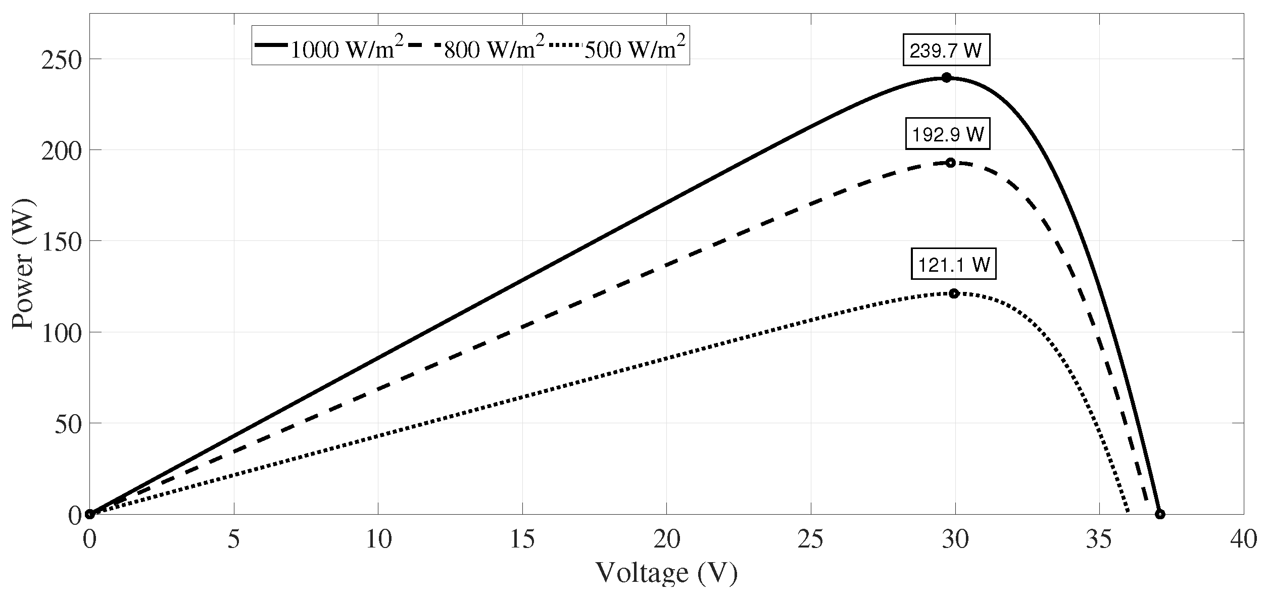
| Maximum power | 239.68 W | |
| Open circuit voltage | 37.1 V | |
| Short-circuit current | 8.58 A | |
| Voltage at MPP | 29.7 V | |
| Current at MPP | 8.07 A |
| Parameter | Description | Value |
|---|---|---|
| Inductor | 0.988 mH | |
| Output capacitor | 1880 F | |
| R | Load resistance | 5 |
Publisher’s Note: MDPI stays neutral with regard to jurisdictional claims in published maps and institutional affiliations. |
© 2022 by the authors. Licensee MDPI, Basel, Switzerland. This article is an open access article distributed under the terms and conditions of the Creative Commons Attribution (CC BY) license (https://creativecommons.org/licenses/by/4.0/).
Share and Cite
Cortes-Vega, D.; Alazki, H.; Rullan-Lara, J.L. Current Sensorless MPPT Control for PV Systems Based on Robust Observer. Appl. Sci. 2022, 12, 4360. https://doi.org/10.3390/app12094360
Cortes-Vega D, Alazki H, Rullan-Lara JL. Current Sensorless MPPT Control for PV Systems Based on Robust Observer. Applied Sciences. 2022; 12(9):4360. https://doi.org/10.3390/app12094360
Chicago/Turabian StyleCortes-Vega, David, Hussain Alazki, and Jose Luis Rullan-Lara. 2022. "Current Sensorless MPPT Control for PV Systems Based on Robust Observer" Applied Sciences 12, no. 9: 4360. https://doi.org/10.3390/app12094360
APA StyleCortes-Vega, D., Alazki, H., & Rullan-Lara, J. L. (2022). Current Sensorless MPPT Control for PV Systems Based on Robust Observer. Applied Sciences, 12(9), 4360. https://doi.org/10.3390/app12094360