
Hourly Power Consumption Forecasting Using RobustSTL and TCN


Abstract
:1. Introduction
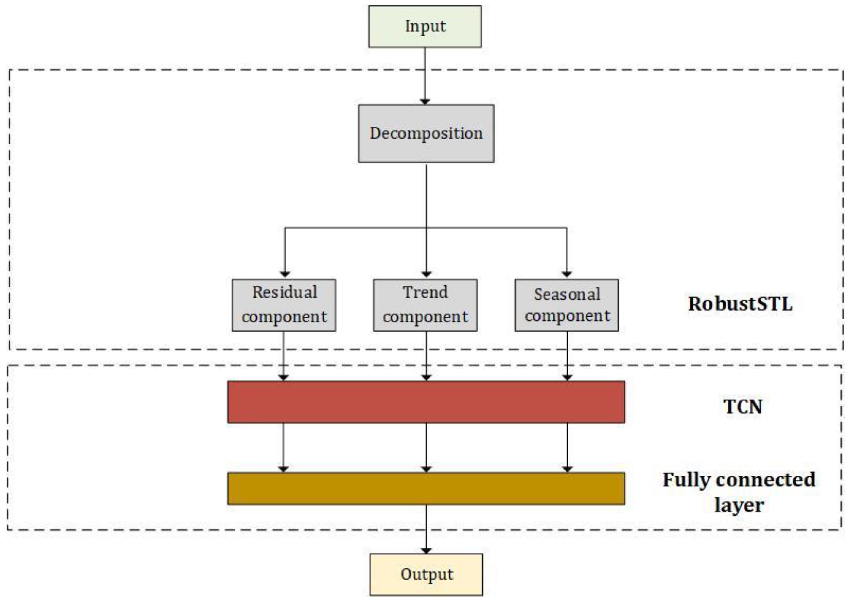
- We propose a forecasting model for single time series data regarding hourly power consumption utilizing RobustSTL and TCN;
- The study’s key contribution is the hybrid model of RobustSTL and TCN as the forecasting model;
- The proposed model can capture and understand the time series data despite containing dynamic patterns and burstiness;
- The experimental stage was performed based on real hourly power consumption and validated with the existing forecasting models.
2. Materials and Methods
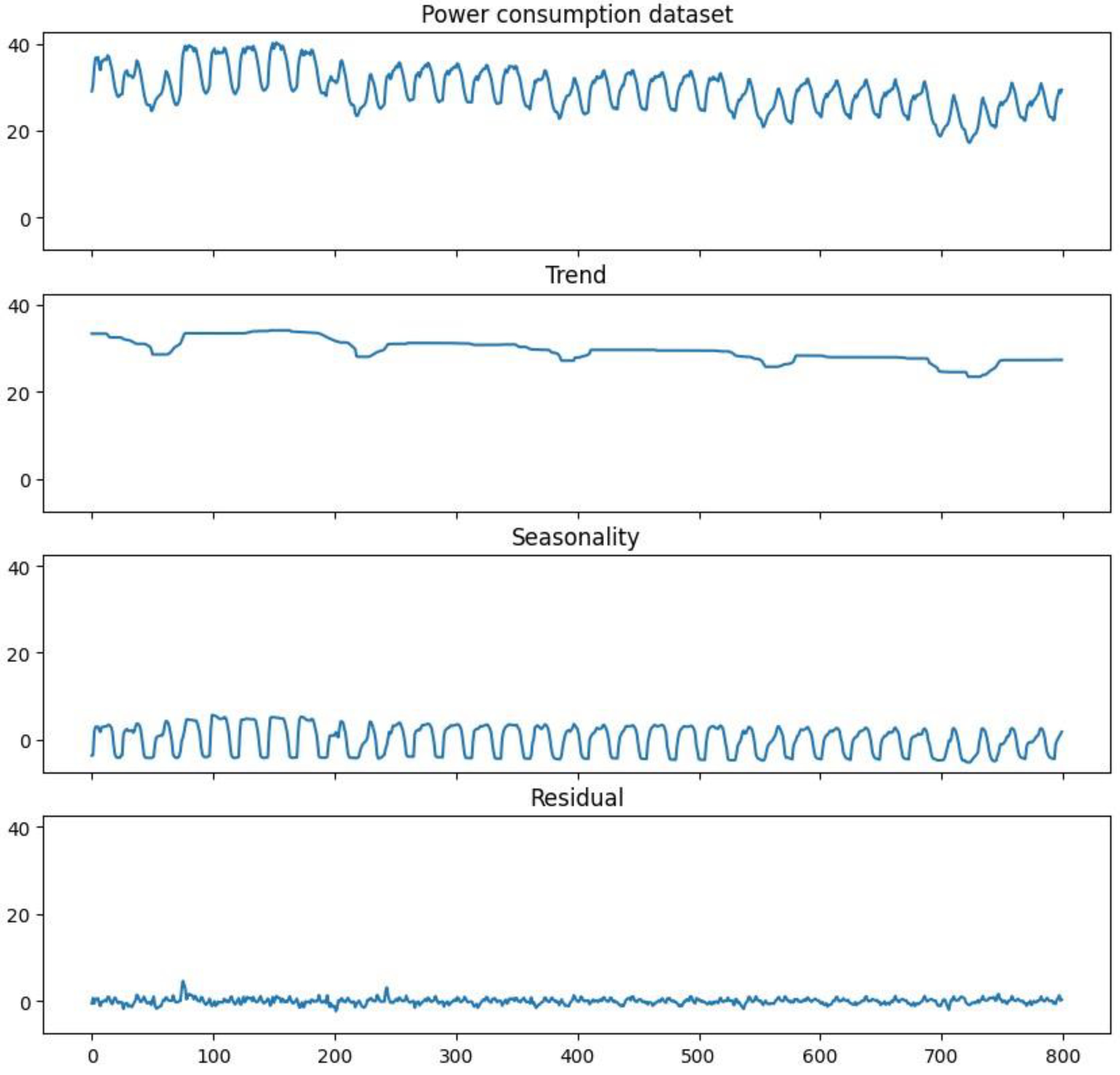
2.1. RobustSTL
| Algorithm 1. RobustSTL method summary |
| Input: yt, parameter configuration |
| Output: τt, st, rt |
| Step 1: Denoise the time series data using bilateral filtering, |
| Step 2: Calculate the relative trend, , |
| Step 3: Calculate the seasonality using non-local seasonal filtering, |
| Step 4: Adjust the trend, seasonality, and remainder components |
| , , |
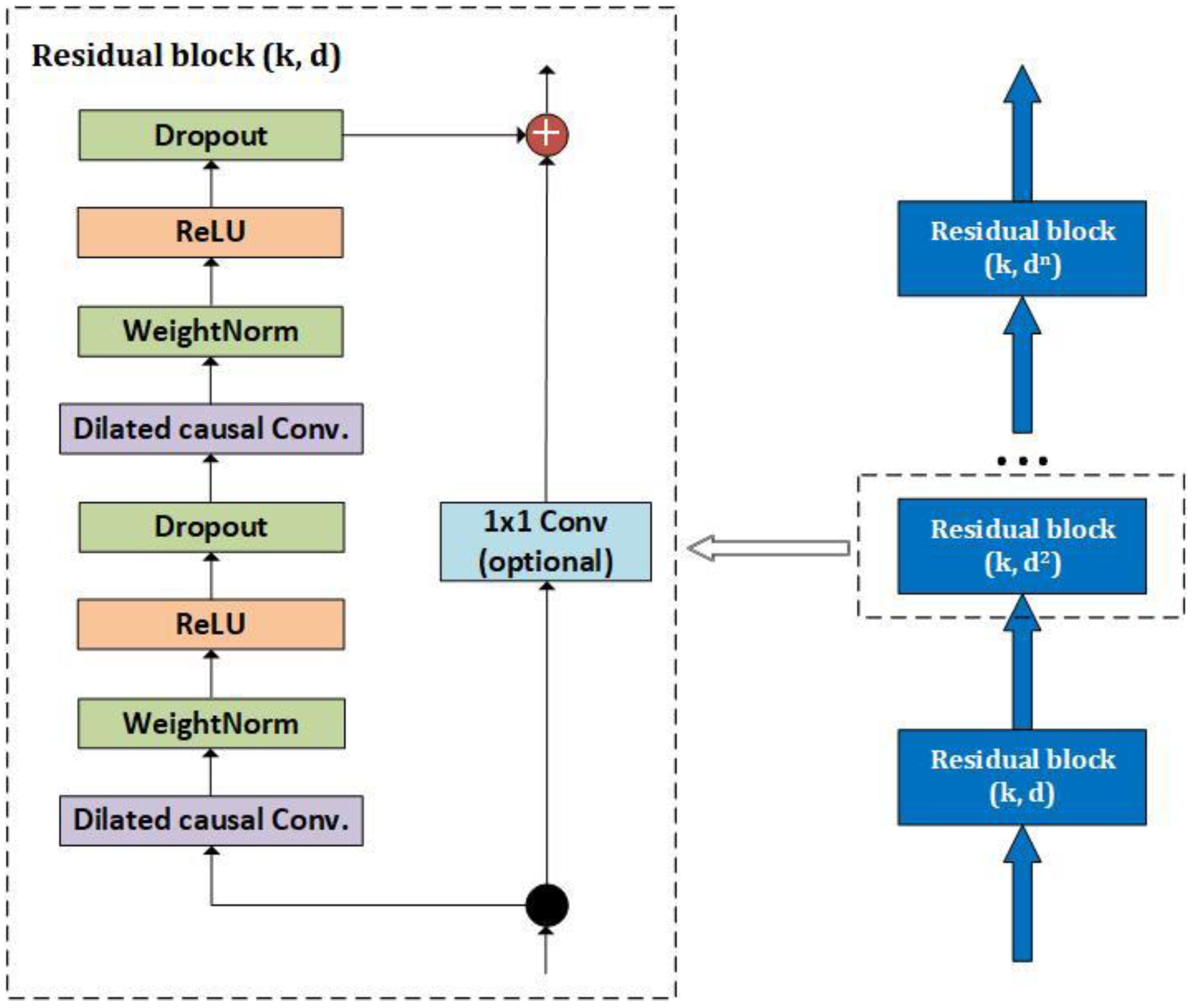
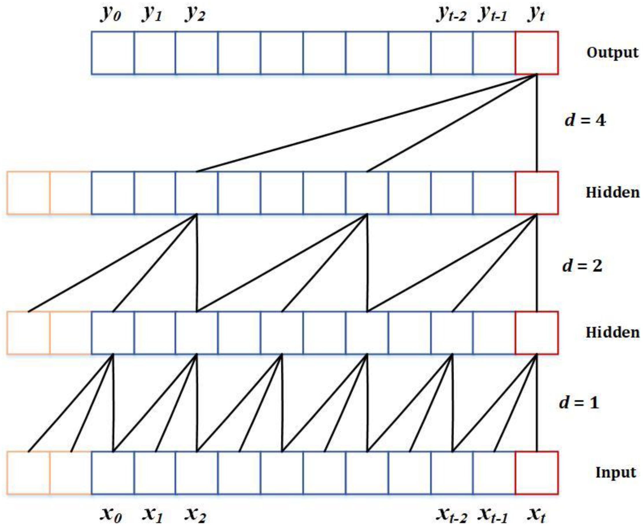
2.2. TCN
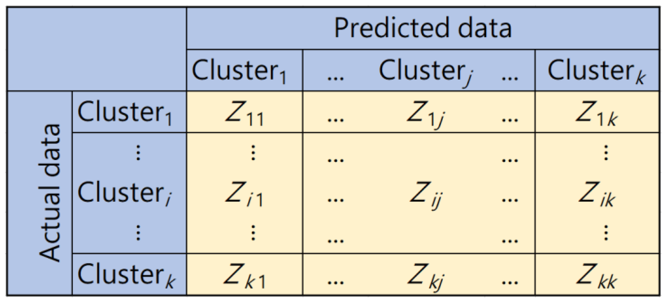
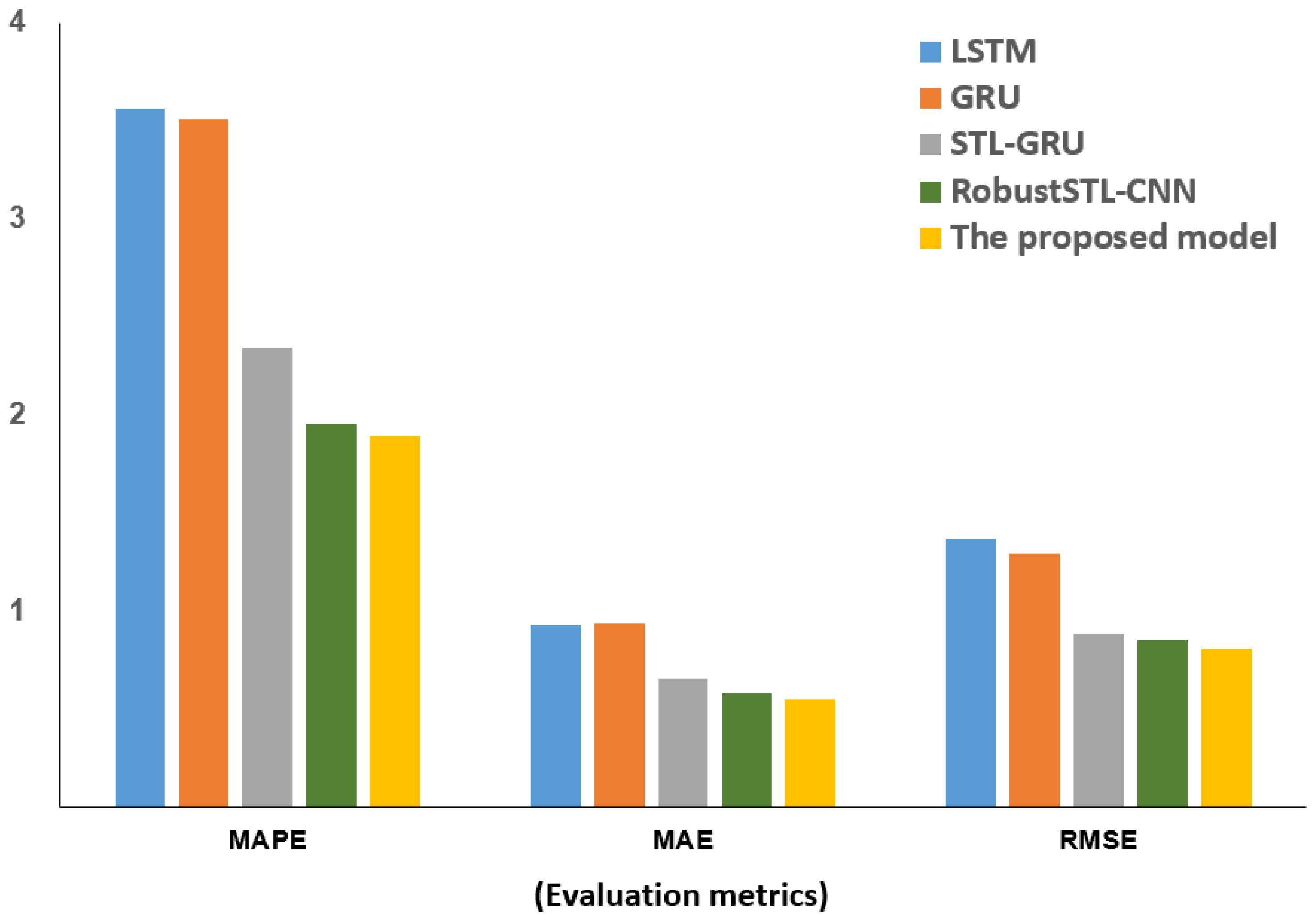
2.3. Evaluation Metrics
3. Results and Discussion
3.1. Data Preparation
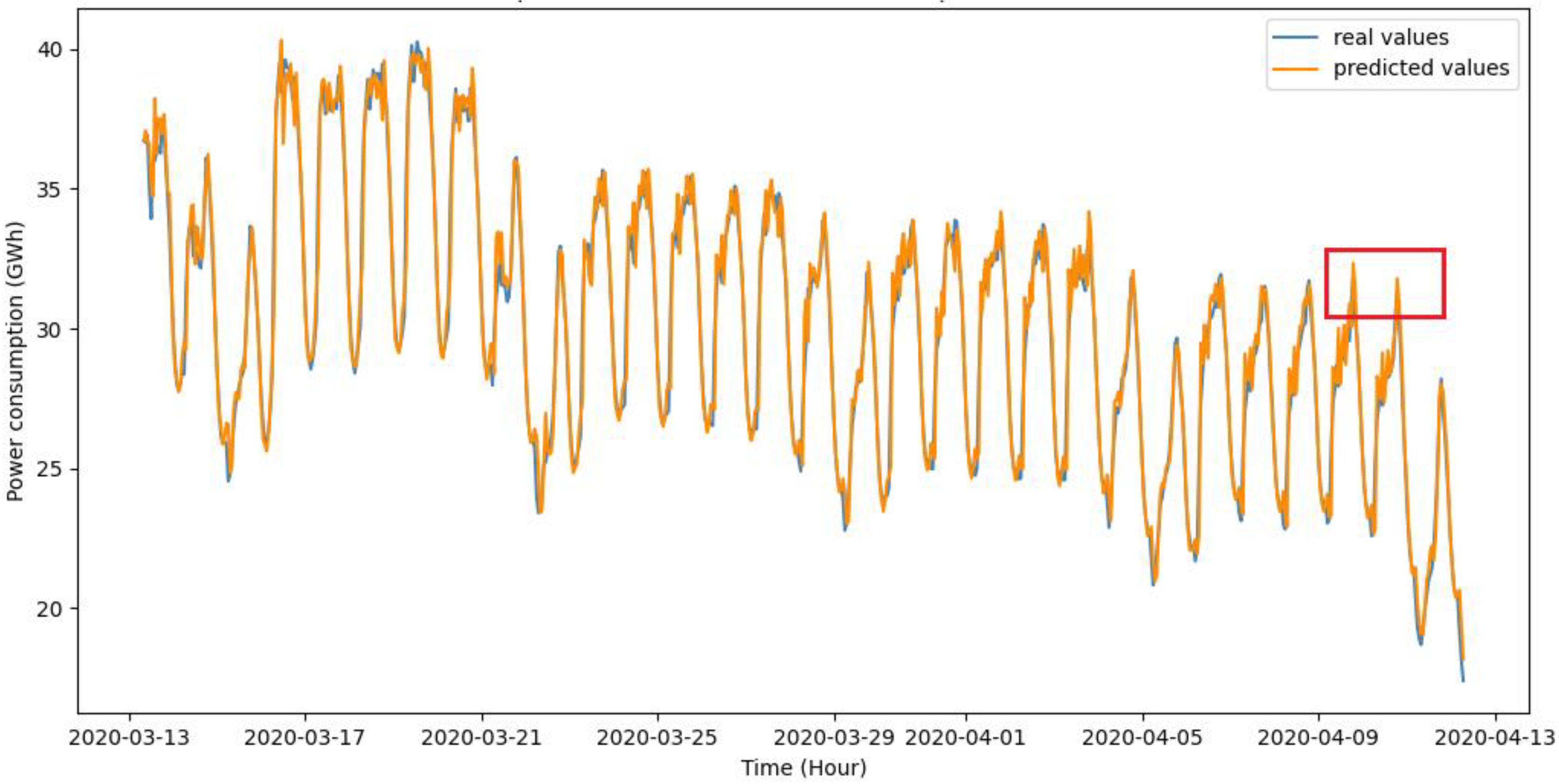
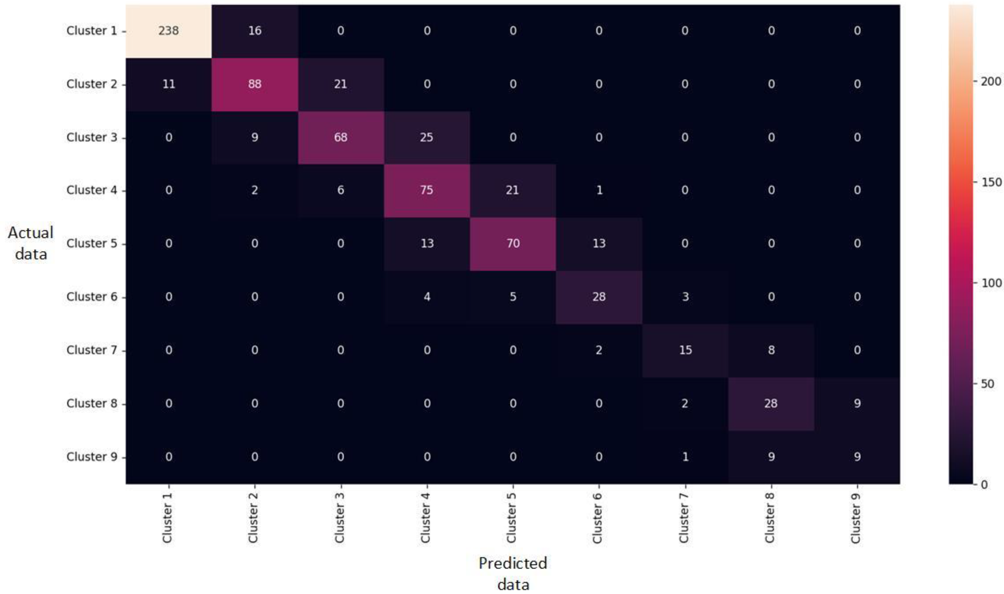
3.2. Experimental Results
4. Conclusions
Author Contributions
Funding
Institutional Review Board Statement
Informed Consent Statement
Data Availability Statement
Conflicts of Interest
References
- Zheng, S.; Huang, G.; Zhou, X.; Zhu, X. Climate-change impacts on electricity demands at a metropolitan scale: A case study of Guangzhou, China. App. Energy 2020, 261, 114295. [Google Scholar] [CrossRef]
- Albuquerque, P.C.; Cajueiro, D.O.; Rossi, M.D.C. Machine learning models for forecasting power electricity consumption using a high dimensional dataset. Expert Sys. App. 2022, 187, 115917. [Google Scholar] [CrossRef]
- Lee, J.; Cho, Y. National-scale electricity peak load forecasting: Traditional, machine learning, or hybrid model. Energy 2022, 239, 122366. [Google Scholar] [CrossRef]
- Petrosanu, D.M. Designing, developing and validating a forecasting method for the month ahead hourly electricity consumption in the case of medium industrial consumers. Processes 2019, 7, 310. [Google Scholar] [CrossRef] [Green Version]
- Sulandari, W.; Subanar; Lee, M.H.; Rodrigues, P.C. Indonesian electricity load forecasting using singular spectrum analysis, fuzzy systems and neural networks. Energy 2020, 190, 116408. [Google Scholar] [CrossRef]
- Fan, M.; Hu, Y.; Zhang, X.; Yin, H.; Yang, Q.; Fan, L. Short-term load forecasting for distribution network using decomposition with ensemble prediction. In Proceedings of the Chinese Automation Congress (CAC), Hangzhou, China, 22–24 November 2019. [Google Scholar]
- Tian, Y.J.; Wen, M.; Li, J.G. A short-term electricity forecasting scheme based on combined GRU model with STL decomposition. In Proceedings of the IOP Conference Series: Earth and Environmental Science, Xi’an, China, 3–6 November 2020. [Google Scholar]
- Mendez-Jimenez, I.; Cardenas-Montes, M. Time series decomposition for improving the forecasting performance of convolutional neural networks. In Proceedings of the Advances in Artificial Intelligence, Granada, Spain, 23–26 October 2018. [Google Scholar]
- Wen, Q.; Gao, J.; Song, X.; Sun, L.; Xu, H.; Zhu, S. RobustSTL: A robust seasonal-trend decomposition algorithm for long time series. In Proceedings of the 33th AAAI Conference on Artificial Intelligence (AAAI-19), Honolulu, HI, USA, 27 January–1 February 2019. [Google Scholar]
- Jiang, F.; Zhang, C.; Sun, S.; Sun, J. Forecasting hourly PM based on deep temporal convolutional neural network and decomposition method. App. Soft Comp. 2021, 113, 107988. [Google Scholar] [CrossRef]
- Wang, Z.; Tian, J.; Fang, H.; Chen, L.; Qin, J. LightLog: A lightweight temporal convolutional network for log anomaly detection on the edge. Comp. Net. 2022, 203, 108616. [Google Scholar] [CrossRef]
- Cleveland, R.B.; Cleveland, W.S.; McRae, J.E.; Terpenning, I. STL: A seasonal-trend decomposition procedure based on Loess. J. Off. Stat. 1990, 6, 3–73. [Google Scholar]
- Bai, S.; Kolter, J.Z.; Koltun, V. An empirical evaluation of generic convolutional and recurrent networks for sequence modeling. arXiv 2018, arXiv:1803.01271. [Google Scholar]
- Yuan, X.; Qi, S.; Wang, Y.; Wang, K.; Yang, C.; Ye, L. Quality variable prediction for nonlinear dynamic industrial processes based on temporal convolutional networks. IEEE Sens. J. 2021, 21, 20493–20503. [Google Scholar] [CrossRef]
- Yin, L.; Xie, J. Multi-feature-scale fusion temporal convolution networks for metal temperature forecasting of ultra-supercritical coal-fired power plant reheater tubes. Energy 2022, 238, 121657. [Google Scholar] [CrossRef]
- Li, J.; Wu, Y.; Li, Y.; Xiang, J.; Zheng, B. The temperature prediction of hydro-generating units based on temporal convolutional network and recurrent neural network. In Proceedings of the 40th Chinese Control Conference (CCC), Shanghai, China, 26–28 July 2021. [Google Scholar]
- Katarya, R.; Verma, O.P. Effectual recommendations using artificial algae algorithm and fuzzy c-mean. Swarm Evol. Comput. 2017, 36, 52–61. [Google Scholar] [CrossRef]
- Deng, X.; Liu, Q.; Deng, Y.; Mahdevan, S. An improved method to construct basic probability assignment based on the confusion matrix for classification problem. Inf. Sci. 2016, 340–341, 250–261. [Google Scholar] [CrossRef]
- Hourly Power Consumption of Turkey (2016–2020). Available online: https://www.kaggle.com/datasets/hgultekin/hourly-power-consumption-of-turkey-20162020 (accessed on 1 November 2021).
- –Namina, S.S.; Tavakoli, N.; Namin, A.S. A Comparison of ARIMA and LSTM in Forecasting Time Series. In Proceedings of the 17th IEEE International Conference on Machine Learning and Applications (ICMLA), Orlando, FL, USA, 17–20 December 2018. [Google Scholar]
- Liu, B.; Fu, C.; Bielefield, A.; Liu, Y.Q. Forecasting of Chinese Primary Energy Consumption in 2021 with GRU Artificial Neural Network. Energies 2017, 10, 1453. [Google Scholar] [CrossRef]
- Yang, S.; Deng, Z.; Li, X.; Zheng, C.; Xi, L.; Zhuang, J.; Zhang, Z.; Zhang, Z. A novel hybrid model based on STL decomposition and one-dimensional convolutional neural networks with positional encoding for significant wave height forecast. Renew. Energy 2021, 173, 531–543. [Google Scholar] [CrossRef]


| Model | MAPE (%) | MAE | RMSE |
|---|---|---|---|
| LSTM | 3.56 | 0.93 | 1.37 |
| GRU | 3.51 | 0.94 | 1.29 |
| STL-GRU | 2.34 | 0.66 | 0.88 |
| RobustSTL-CNN | 1.95 | 0.58 | 0.85 |
| The proposed model | 1.89 | 0.55 | 0.81 |
| Model | Precision | Recall | F1-Score |
|---|---|---|---|
| LSTM | 0.65 | 0.64 | 0.64 |
| GRU | 0.61 | 0.63 | 0.62 |
| STL-GRU | 0.60 | 0.61 | 0.60 |
| RobustSTL-CNN | 0.63 | 0.62 | 0.62 |
| The proposed model | 0.70 | 0.70 | 0.70 |
Publisher’s Note: MDPI stays neutral with regard to jurisdictional claims in published maps and institutional affiliations. |
© 2022 by the authors. Licensee MDPI, Basel, Switzerland. This article is an open access article distributed under the terms and conditions of the Creative Commons Attribution (CC BY) license (https://creativecommons.org/licenses/by/4.0/).
Share and Cite
Lin, C.-H.; Nuha, U.; Lin, G.-Z.; Lee, T.-F. Hourly Power Consumption Forecasting Using RobustSTL and TCN. Appl. Sci. 2022, 12, 4331. https://doi.org/10.3390/app12094331
Lin C-H, Nuha U, Lin G-Z, Lee T-F. Hourly Power Consumption Forecasting Using RobustSTL and TCN. Applied Sciences. 2022; 12(9):4331. https://doi.org/10.3390/app12094331
Chicago/Turabian StyleLin, Chih-Hsueh, Ulin Nuha, Guang-Zhi Lin, and Tsair-Fwu Lee. 2022. "Hourly Power Consumption Forecasting Using RobustSTL and TCN" Applied Sciences 12, no. 9: 4331. https://doi.org/10.3390/app12094331
APA StyleLin, C.-H., Nuha, U., Lin, G.-Z., & Lee, T.-F. (2022). Hourly Power Consumption Forecasting Using RobustSTL and TCN. Applied Sciences, 12(9), 4331. https://doi.org/10.3390/app12094331