Applying a Deep Learning Neural Network to Gait-Based Pedestrian Automatic Detection and Recognition

Abstract

Gait recognition is a noncontact biometric procedure that determines the identity or health status of a person by analyzing his or her walking posture and habits, including skeletal and joint movements. The most remarkable feature of this method is the possibility of conducting recognition without demanding much cooperation from participants. Therefore, this recognition technique has attracted much attention from scholars. Additionally, because of the rapid development of graphics processing unit technology, related hardware and computation performance, the applications of deep-learning technology are considerably enhanced. The objective of this study was to apply a deep neural network (DNN), which employs deep-learning technology, to achieve gait-based automatic pedestrian detection and recognition. In contrast to using wearable devices to precisely capture skeletal and joint movements, pedestrian color-image sequences were used as input in this study. Subsequently, a pretraining convolutional neural network (CNN) was employed to capture pedestrian location and extract pedestrian dense optical flow to serve as concrete low-level feature inputs. Then, a finely-tuned DNN based on the wide residual network was employed to extract high-level abstract features. In addition, to overcome the difficulty of obtaining local temporal features by using a 2D CNN, part of the 3D convolutional structure was introduced into the CNN. This design enabled use of limited memory to acquire more effective features and enhance the DNN performance. The experimental results show that the proposed method has exceptional performance for pedestrian detection and recognition.

1. Introduction

In recent years, because of the rapid development of graphics processing unit (GPU) technology, hardware and computation performance in the research and application of artificial intelligence have improved considerably. Accordingly, machine learning technologies based on neural networks (NNs) have also seen rapid advancement. Common NNs include the recurrent NN, which is suitable for handling tasks in a specific context, and convolutional NN (CNN), which is suitable for image processing. Evidence has shown that NNs with deep-learning technology excel at classification tasks. Moreover, such NNs can achieve exceptional results in research and application in various fields through design of a suitable NN framework based on the task features, so long as the task in question can be transformed into a classification task. In particular, biometric identification is the primary field exhibiting marked development in the use of NN technology.

In contrast to conventional handcrafted features, which are intuitive and observable by human eyes, higher level abstract features extracted using deep learning NNs contain extremely detailed information that is difficult for humans to understand, particularly the features acquired from deep NN.

Regarding biometrics, gait recognition refers to the analysis of pedestrians’ walking habits and postures to obtain a variety of information. Depending on the features of the task at hand, gait data can be obtained by observing and recording skeletal movements with instruments, such as wearable devices and multiple cameras, and through clinical measurement or analyses of image sequences to identify a specific pedestrian. Moreover, in contrast to other biometric identification such as iris recognition and fingerprint recognition—both of which require collecting biometric data from users—gait-based pedestrian recognition does not require collaboration from pedestrians in biometric feature collection because cameras are set up at a distance. Moreover, habitual movements are difficult to alter over a short period. Therefore, gait-based pedestrian recognition is not subject to changes in appearance (e.g., face coverage or outfit change) and is considerably more applicable to security systems—such as surveillance cameras—than is facial recognition, which requires complete facial images. Numerous scholars have conducted research on this topic in recent years.

Gait recognition is similar to activity recognition, which involves series of analyses of human action sequences. Therefore, dense optical flow, which is often used in activity recognition, is considered effective in gait recognition. Dense optical flow eliminates back-ground influences and effectively captures low-level features of pedestrian activities.

A deep-learning NN was applied in this study to analyze pedestrian gait, and high-level abstract features of walking manners were extracted to conduct biometric recognition tasks. This study incorporated deep-learning NNs to conduct gait recognition. Such NNs include the pretrained NN, which extracts dense optical flow. This process obtained the moving speed of pixels between two consecutive images in a color pedestrian image sequence and eliminated influence from appearance features and backgrounds. Subsequently, a pedestrian detection NN was applied to obtain pedestrian location by focusing on the region of the pedestrian in question. By processing a sizable gait database, this study obtained a sufficient number of samples to train a deep learning NN that can effectively extract pedestrian gait features. This was followed by verification of the performance and reliability of the deep-learning NN.

Research on gait analysis and recognition methods has involved various aspects such as portrait segmentation and skeleton tracking, which are similar to activity recognition [1,2]. Favorable outcomes have been achieved on activity recognition by inputting the RGB color model and optical flow into the NN. Additionally, studies such as [3,4] have applied the recurrent NN recognition method based on time sequences. In particular, [3] adopted long short-term Memory (LSTM), whereas [4] converted the convolution kernel in the standard CNN framework to a three-dimensional (3D) structure. However, compared with activity recognition, differences observed during gait recognition are extremely subtle. Consequently, gait recognition entails discarding intuitively or visually identifiable appearance cues to prevent changes in appearance from affecting the recognition results.

Studies regarding other gait recognition methods involving NNs included the following. In [5], the CNN was applied to estimate posture in images to obtain the location of each body part, in order to input the observed sequence into LSTM for distinction. In [6], sensors were applied on human bodies to track the up–down oscillation of five body parts including the waist and hand; subsequently, the collected data were compiled to be inputted into the NN. In [7], the silhouette-based method was employed; this method captures joints such as the pelvis, waist, neck, and knees from the partitions of a silhouette and trains the NN using data on the relative locations of these joints. In [8], after computation of an individual’s optical flow, each body part that moved considerably while walking, such as the pelvis (including arm movement), legs, upper body, and lower body, was tracked; subsequently, the optical flow of each body part (the length and width of the input of each part were adjusted to 48 × 48) was inputted into the NN to enhance performance. In [9], the optical flow of a segment of a complete image was employed instead of purposely capturing images of pedestrians, and the complete displacement of the pedestrian in the image was visible. This method reduced the length and width of the data to 1/8 of the original data for NN input; in addition, four CNNs with different convolution kernel scales were employed.

The present study employed the DNN to detect the region where a pedestrian in an image was located. This region was then set as the region of interest (ROI) and its coordinates were sent to the optical flow sequence to capture the ROIs of pedestrians in the corresponding optical flow. In addition, the wide residual networks (Wide ResNet) framework, featuring an exceptional performance and training rate, was employed as the foundation for minor modification. Then, a 3D convolution structure was concatenated at the front to establish a gait feature extraction DNN with optimal representation.

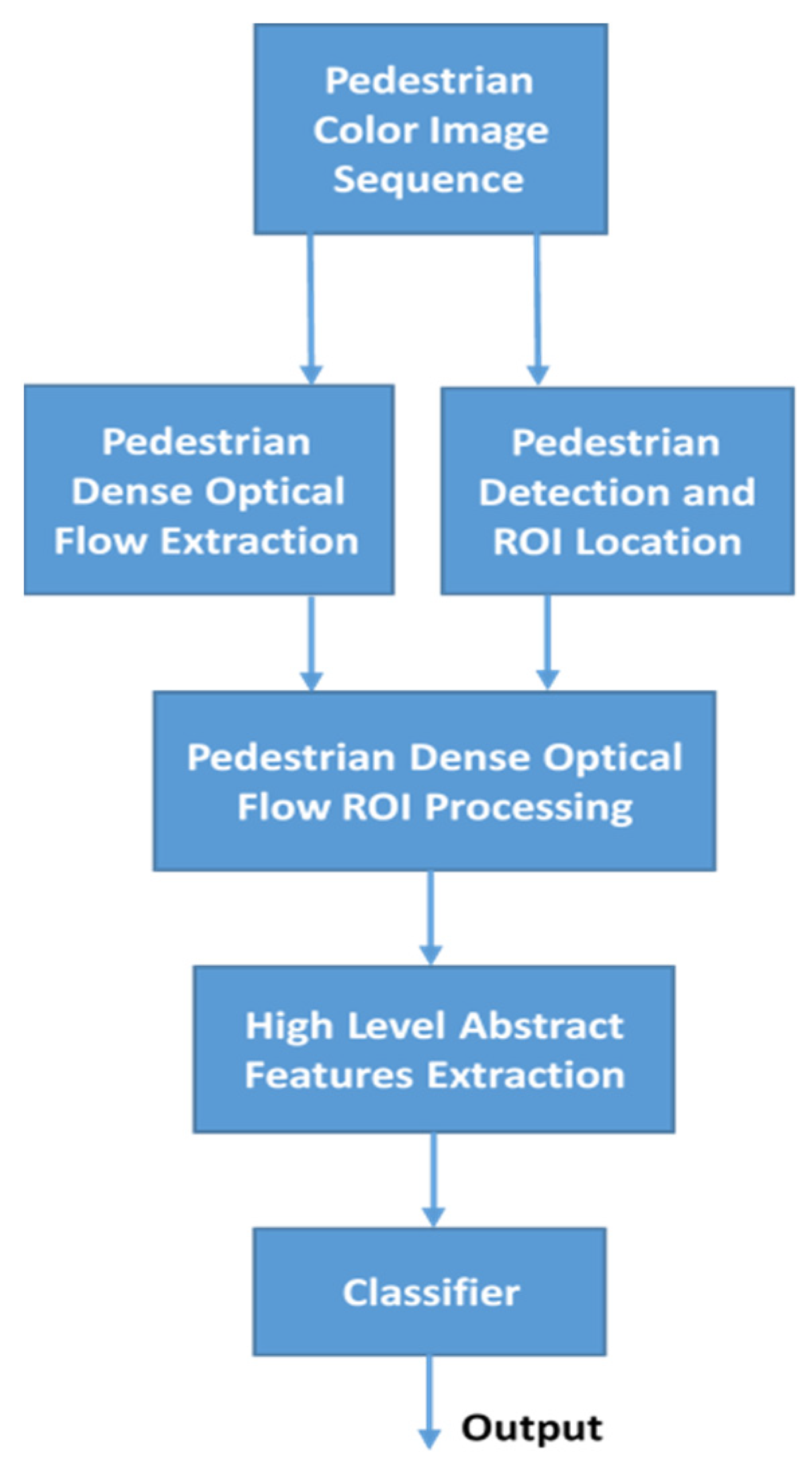
This study established a pedestrian recognition method involving pedestrian gait analysis using dense optical flow and pedestrian detection. The flowchart of this method is presented in Figure 1. Items in this flowchart include pedestrian dense optical flow, tracking pedestrian location and capturing pedestrian ROI, the NN that captures high-level abstract features, and a classifier.

The first input contained a set of pedestrian color image sequences with n images. Subsequently, two pretraining DNNs, namely YOLOv2 [10] and FlowNet2.0 [11], were applied to track the bounding box of pedestrian location and generate dense optical flow (total of n − 1) from each pair of two consecutive images. The obtained pedestrian location border was applied to determine the complete pedestrian ROI (PROI). The PROI location data was then applied to the pedestrian optical flow data. Subsequently, the background region where no pedestrian optical flow had been detected was discarded from the captured PROI of the optical flow to reduce the size of the optical flow. Then, the obtained pedestrian optical flow was aligned centrally to facilitate zero-padding in the surrounding area until the maximal border (H length and W width) was reached. The ROIs of the processed pedestrian optical flows were concatenated to form an optical flow sequence of size H × W pixels that would be inputted into the DNN to capture high-level abstract features. Finally, the captured high-level abstract features were inputted into the classifier for recognition. The outcome was the recognition results of the initial input.

2. Pedestrian Color Image Sequence

The TUM-GAID Gait Dataset [1] is a pedestrian gait dataset maintained by Kinect that contains raw color image sequences and corresponding depth map sequences; the raw resolution is 640 × 480 pixels.

This dataset initially contained gait sequences of 305 pedestrians. These image sequences comprised two trajectories, namely left to right and right to left. In addition, each pedestrian had his or her own scenario, described as follows:

• Normal clothing (regular daytime outfit; marked as “N” for normal): Six sequences, namely walking three times from left to right and three times from right to left.
• Backpack (addition of a backpack weighing approximately 5 kg; marked as “B” for backpack): Two sequences, namely walking once from left to right and once from right to left.
• Shoe covers (addition of white shoe covers to the original shoes; marked as “S” for shoe covers): Two sequences, namely walking once from left to right and once from right to left.
• Seasonal clothing (documented at various times with notably different clothing; marked as “TN” for elapsed time—normal): Six sequences, namely walking three times from left to right and three times from right to left.
• Seasonal clothing + backpack (marked as “TB”): Two sequences, namely walking once from left to right and once from right to left.
• Seasonal clothing + shoe covers (marked as “TS”): Two sequences, namely walking once from left to right and once from right to left.

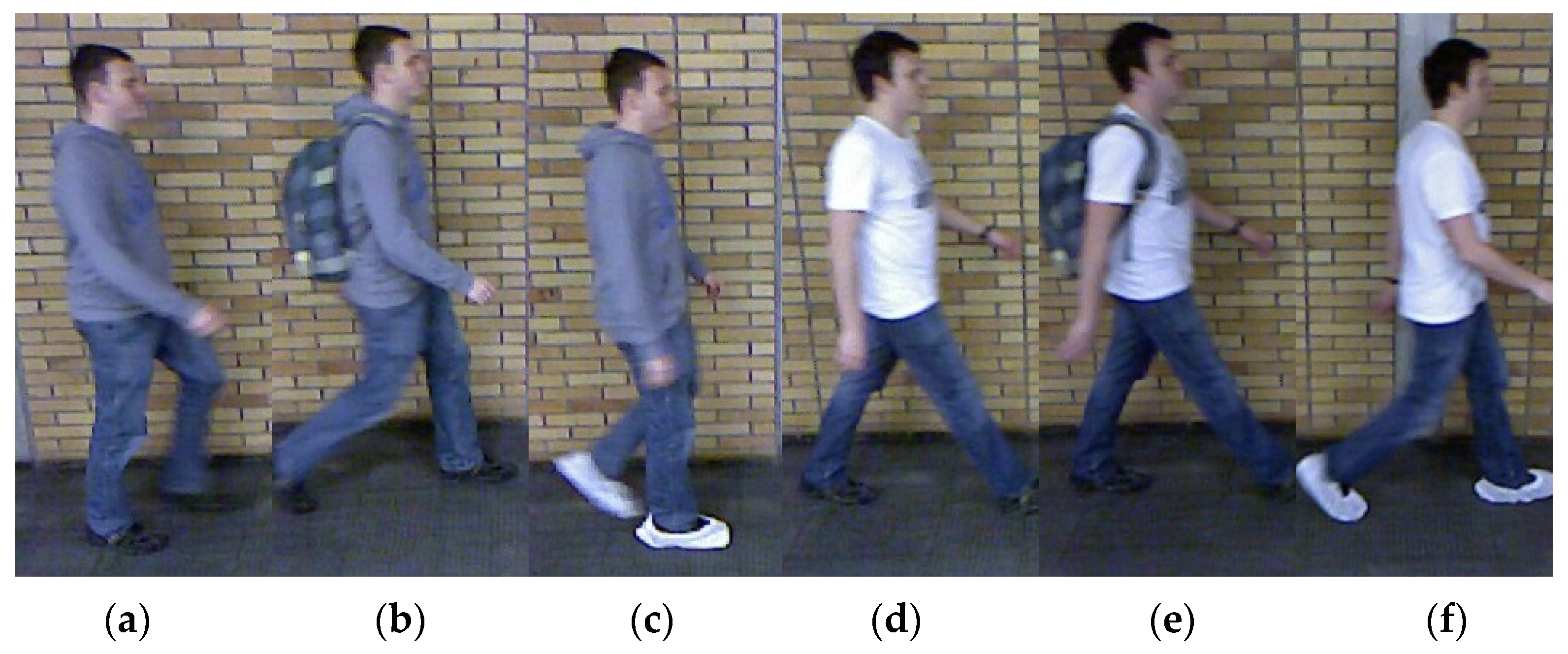
As shown is Figure 2, each pedestrian had at least six N sequences (N1, N2, … N6), two B sequences (B1 and B2), and two S sequences (S1 and S2) documented. Subsequently, 32 pedestrians participated in documentation in multiple seasons; thus, an additional eight sequences marked as TN, TB, and TS were documented for these participants. In total, the dataset currently contains more than 3000 pedestrian sequences. Each sequence spans 1 to 2 s (approximately 30 frames per second) and contains 60 to 90 frames.

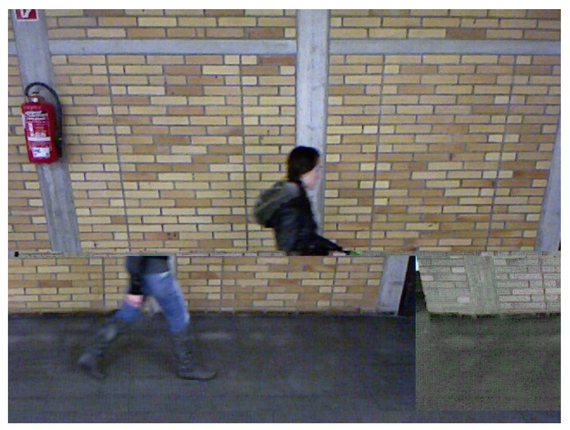
At the beginning and end of each sequence, where the pedestrian entered and exited the screen, respectively, most of his or her body was cropped. Although the pedestrian-tracking NN was able to detect the pedestrian, the present study eliminated the first and final five frames of each sequence for the integrity of the pedestrian. In addition, misaligned images shown in Figure 3 caused by the equipment were discarded. Misalignment resulted in a considerable number of unlikely values generated from the captured optical flow value such as sudden displacement of more than 100 pixels. After such misaligned images had been discarded, the horizontal and vertical moving speeds mostly fell within the reasonable range.

3. Pedestrian Detection and ROI Location

Observation of a complete raw color image revealed that the background, which did not move, accounted for a large part of the image and would result in redundant computation during subsequent NN training. Furthermore, non-pedestrian regions or objects in the background would cause interference. To eliminate excessive input and focus the analysis on the pedestrians, a pretraining NN for object detection, namely YOLOv2, was introduced to detect pedestrian location. This NN captured PROIs from image sequences.

Object detection is a common problem in the CNN framework. Object detection methods involving NNs are many in number. Better-known methods include the two-stage R-CNN series and YOLO, the NN with an end-to-end framework [12]. The logic and technology of YOLO and the improved YOLOv2 [10] are described as follows.

The R-CNN series employs a region proposal as its logical basis. Initially, a high number of possible bounding boxes is generated. Then, a classifier is applied to discriminate the content of these bounding boxes. Finally, postprocessing is conducted to eliminate repeated bounding boxes and retain the optimal solution. The subsequently developed Fast R-CNN [13] and Faster R-CNN [14] inherited the same logic and integrate various network models used over multiple stages into one unified NN. Finally, two main NNs are generated, namely the region proposal network and classification network.

Compared with the R-CNN series, YOLO regards the detection problem as a regression problem and combines the processes of predicting bounding and objects into a single NN. In addition, YOLO conducts image prediction based on the entire image. Therefore, compared with the R-CNN, the rate of mistaking the background as an object can be reduced by more than 50%. Moreover, evaluation of plural candidate frame areas is no longer required, and thus speed and generalizability are improved.

4. Pedestrian Dense Optical Flow Extraction

Optical flow refers to the instantaneous velocity of the motion of each pixel in an image plane during the movement of an object. Correlation of two frames in this moving sequence is necessary to compute the offset of the object in two consecutive frames. Dense optical flow is an image comparison method that uses point-to-point matching of images. Compared with sparse optical flow, which compares only several feature points in an image, dense optical flow computes all pixel offsets in an image. To eliminate excessive information that the NN does not require such as background and pedestrian appearance—including colors of clothes and shifts between light and shadow—the present study set pedestrian movement as the focal point. In particular, gait sequences were described by capturing dense optical flow from two color images.

In this study, the DNN used to capture dense optical flow was a variant of the fully convolutional network (FCN) framework called FlowNet2.0. The FCN was first introduced in [15] to solve a problem that the original CNN framework could not solve, namely recognizing an object at a particular location or a particular part of an image. Although the CNN framework is suitable for classifying a complete image, it cannot identify possible sub-elements in the image. Therefore, the FCN was introduced to solve such problems.

The fundamental CNN usually flattens an entire image into a one-dimensional vector after classifying the convolution layer, followed by classification at the fully connected layer by using the Softmax function. The fundamental concept of the FCN is to classify each pixel in an image to achieve pixel-level image segmentation. Specifically, the FCN replaced the fully connected layer with a convolution layer. Therefore, the end result of the NN was an unflattened high-dimensional feature map. Another benefit of replacing the fully connected layer with a convolution layer is the possibility of sliding on large input images; the outcomes obtained from each location where the convolution kernel slid were the classification results of said locations in this study.

FlowNet [16] operates by training an FCN and obtaining pixel-level optical flow in an image sequence. This method is based on two basic NNs, namely FlowNetS and FlowNetC, as well as a refinement. The main difference between FlowNetS and FlowNetC is that FlowNetS concatenates two consecutive frames for input, whereas FlowNetC separately inputs two image frames through three convolution layers before conducting correlation analysis on the two frames and calculating the relationship between the two feature maps. For single network operations, FlowNetC is superior to FlowNetS. The refinement section is a network that uses deconvolution to obtain the final optical flow, and employs bilinear interpolation, which requires relatively few computational resources yet does not cause considerable differences in results. Moreover, to not lose details, the deconvolution process concatenates the convolution result with the previous deconvolution prediction result.

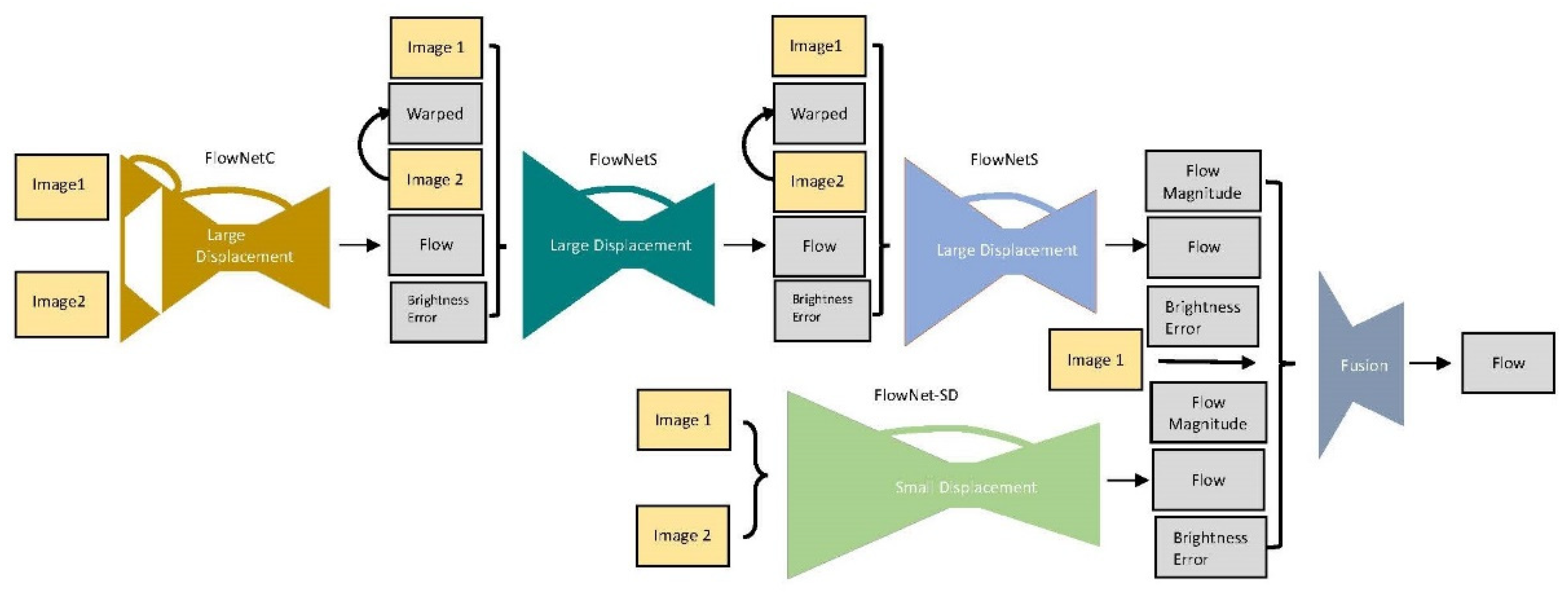
Because the results of using only FlowNetS or FlowNetC for training could still be improved, a follow-up study [11] concatenated these networks. Consequently, FlowNet2.0 with enhanced performance was developed; its network structure is presented in Figure 4 which was redrawn based on the information in [11].

Because FlowNetC is more accurate but FlowNetS can more easily replace an input, the first network was set as FlowNetC. Subsequently, bilinear interpolation was applied to the second frame and the result of the first network to calculate warping. Then, the brightness error was added as the input for the next network, namely FlowNetS. Because bilinear interpolation is suitable for computation of the gradient, the aforementioned three networks could be combined; this combination was named FlowNet-CSS.

The original network was not sensitive to extremely low displacement, which is disadvantageous in processing of real-world data. Therefore, in [11], a dataset of low displacement data was employed to conduct fine tuning and obtain a low displacement network. Finally, the results from the two networks were inputted into the fusion network to obtain the final NN, namely FlowNet2.0. This network benefits from the advantage of effective GPU computation, which enables marked improvement in computation speed and generates results similar to those of most advanced conventional handcrafted feature methods such as FlowFields [11]. Therefore, the present study employed FlowNet2.0 to capture the pedestrian dense optical flow.

5. Pedestrian Dense Optical Flow ROI Processing

The pedestrian dense optical flow of the entire image obtained by FlowNet2.0 revealed that a large part of the optical flow consisted of immobile backgrounds, which could have caused excessive computation or even interference in the subsequent NN training and recognition. To eliminate excessive background areas and focus the analysis on pedestrians, a YOLOv2 object detection NN was employed to detect pedestrian location. Subsequently, the PROI was captured from the corresponding pedestrian dense optical flow, and the background region where no pedestrian optical flow was detected was discarded to reduce the optical flow size. Then, the obtained pedestrian optical flow was aligned centrally to facilitate zero-padding on the surrounding area until the maximal border (H length and W width) was reached. Through this method, the raw pedestrian color image was converted into a pedestrian optical flow ROI sequence.

To facilitate batch training, the size of all optical flow input was set to 304 × 480 pixels, and all values were normalized to the interval of [0, 1]. However, this size was still a considerable burden for the training network. According to [8,9], low resolution can achieve similar effects while accelerating the training process. In contrast to [9], which reduced the size of raw images, the present study reduced the optical flow size to one-eighth of the original size (38 × 60). 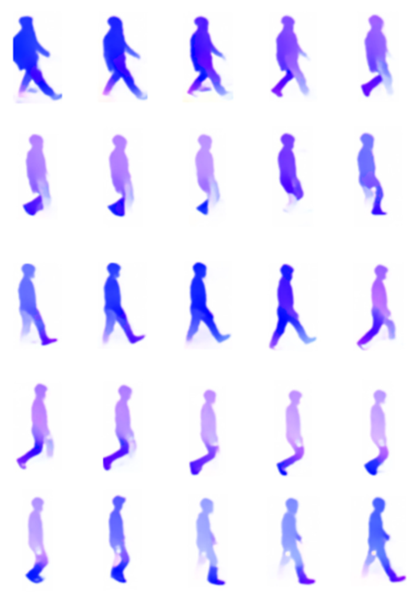Figure 5 presents the results of the encoded PROI captured from the optical flow, which was captured by the optical flow-capturing NN mapped onto the color image space.

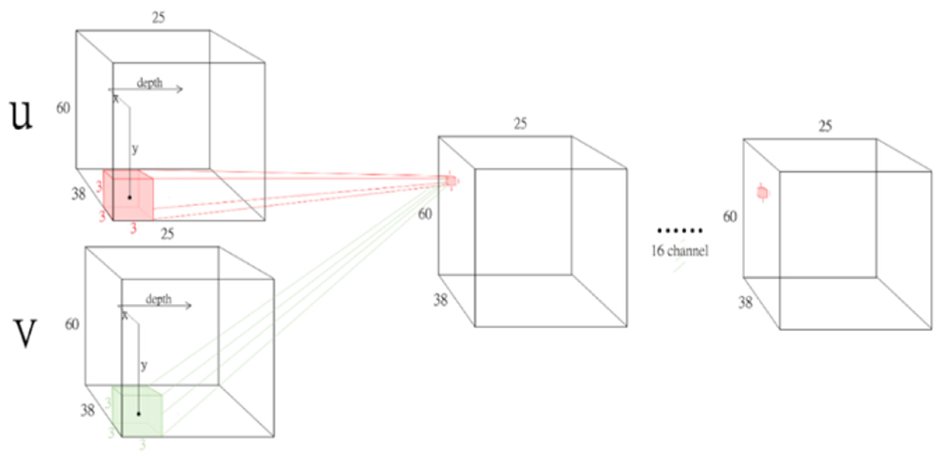
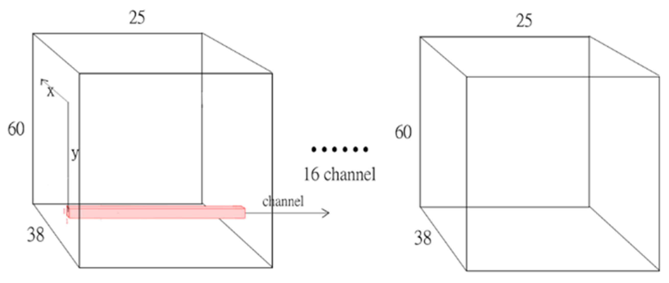
According to the training strategy and actual observation dataset in [9], the walking cycle of a pedestrian is approximately 25 frames per cycle. Therefore, every 25 frames from the processed pedestrian optical flow sequence were taken as a sample and each sample was taken five frames apart. Eight to twelve samples were taken from each sequence and the total number of samples was 26,948. Each optical flow contained two channels of directional displacement velocity, namely the x-direction displacement at velocity u and y-direction displacement at velocity v. Therefore, an input of size 38 length × 60 width × 50 channels was obtained for each sample.

At the input stage, samples were processed by one-hot encoding (305 pedestrians coded from 0 to 304) to obtain the same number of dimensional vectors as that of pedestrian optical flow samples. Each dimension represented the probability of a specific pedestrian. The correct dimension was marked 1.0 and all others were marked 0.0. For example, if one ground truth was tagged No. 25, one-hot encoding would obtain a 305-dimensional vector where the vector with an index of 25 would be marked 1.0, and all others would be marked 0.0.

The 26,948 samples were divided into a training set and testing set. This study established the following experimental plans:

• All samples were randomly distributed at a 7:3 ratio to yield 18,978 training samples and 7970 testing samples.
• All samples were randomly distributed at a 5:5 ratio to yield 13,558 training samples and 13,390 testing samples.

6. High-Level Abstract-Feature Extraction

To obtain further pedestrian motion feature data from the captured pedestrian dense optical flow ROI, a new NN needed to be trained to perform higher level abstract feature extraction. To achieve rapid training and exceptional performance, this study employed the Wide ResNet structure as its fundamental model. Compared with the VGG-like structural model, the Wide ResNet structure is easier to train, is quicker to converge, and has fewer parameters; moreover, its structure is simple. Because of the lack of a fully connected layer, the limitation on input size is low, and thus conducting fine tuning on a multiscale input in the NN is easier. Additionally, the Wide ResNet structure is more effective than residual networks (ResNet) [17]. The present study introduced the predecessor to Wide ResNet, namely ResNet, by explaining the influence of the residual block on NN design before presenting Wide ResNet and its improvements.

6.1. Wide Residual Network (Wide ResNet)

Numerous variants of ResNet have been developed; one of the most popular of these is Wide ResNet. ResNet [17] focused on the effect of NN depth on accuracy, whereas Wide ResNet [18] determines the effect of NN width on accuracy.

In [18], the researchers indicated that in an overly deep NN, some residual blocks were unable to provide feature data or only some residual blocks could learn key feature data. In other words, a large number of residual blocks in an overly deep network had no actual function but rather caused redundant computation. Wide ResNet reduced the depth of networks and widened the number (width) of convolution kernels in residual blocks for verification. The ResNet and Wide ResNet designs [18] are compared in Figure 6 which was redrawn based on the information in [18].

ResNet contains more than 50 layers of models. To reduce the number of model parameters, a bottleneck design was employed to replace two 3 × 3 convolution kernels with a 3 × 3 convolution kernel that had two 1 × 1 convolution kernels clipped onto it. However, to test the effect of width on this design [18], as shown in

Table 1. Basic structure of Wide Resnet.

Group Name	Output Size	Block Type = B(3,3)
conv1	32 × 32	[3 × 3, 16]
conv2	32 × 32	$\left[\begin{array}{c}3\times 3,16\times \mathrm{k}\\ 3\times 3,16\times \mathrm{k}\end{array}\right]\times \mathrm{N}$
conv3	16 × 16	$\left[\begin{array}{c}3\times 3,32\times \mathrm{k}\\ 3\times 3,32\times \mathrm{k}\end{array}\right]\times \mathrm{N}$
conv4	8 × 8	$\left[\begin{array}{c}3\times 3,64\times \mathrm{k}\\ 3\times 3,64\times \mathrm{k}\end{array}\right]\times \mathrm{N}$
avg-pool	1 × 1	[8 × 8]

that adopted the data in [18], the researchers still employed two 3 × 3 convolution kernels. In addition, to impede overfitting as the number of parameters increased, a dropout layer was added between any two consecutive layers. Based on this structure, two parameters were proposed, namely the number of residual blocks (N) and the number of times that convolution kernels are widened (K).

In [18], experiments on residual blocks composed of multiple combinations of convolution kernels were conducted and optimal results were obtained from the basic B(3,3) framework. Adding more layers or incorporating the bottleneck structure yielded testing outcomes with higher error occurrence or no performance improvement; by contrast, adding a dropout layer engendered notable effects. For more information about Wide ResNet, refer to [18].

6.2. Wide ResNet Modification

Because of its advantages, the present study employed Wide ResNet as the foundation to extract high-level abstract features. The residual block kernel consisted of the B(3,3) structure with dropout layers. In addition, the order of batch normalization, activation, and the conv layer was altered from that established in [18] from conv layer, activation, batch normalization to batch normalization, activation, conv layer. The modified Wide ResNet structure is detailed in

Table 2. Modified Wide Resnet structure.

Group Name	Kernel Size	Output Size (Batch,Height,Width,Channel)	Note
Input		(Batch,60,38,50)
Initial Conv2d	3	(Batch,60,38,32)	Stride = 1
Res Group 01	3	(Batch,60,38,16k)	N = 2 k = 4 Drop rate = 0.3
Res Group 02	3	(Batch,30,19,32k)
Res Group 03	3	(Batch,15,19,64k)
Batch Normalization
Activation function
Global Average Pooling	[15 × 19]	(Batch,1,1,64k)

.

The settings of the other global hyperparameters were as follows:

• Batch Normalization Layer, Momentum = 0.99
• Dropout Layer, Drop rate = 0.3
• Activation Function = LeakyReLU, Equation (1)

$$\mathrm{f}\left(\mathrm{x}\right)=\{\begin{array}{cc}\mathrm{x}& \mathrm{when}\mathrm{x}>0\\ \mathsf{\alpha }\mathrm{x}& \mathrm{when}\mathrm{x}\le 0\end{array}$$

(1)

where α > 0 and α ∈ R.

According to each task, the hyperparameters and parts of the network structure of a deep-learning CNN should be modified to achieve the optimal effect. The present study determined several methods for modifying the Wide ResNet model and added an extra 3D convolution layer to enhance the representation of the temporal feature.

6.2.1. NN Width Modification and Batch Training Size

The fundamental factor affecting NN performance was the number of parameters, and the usual approach to raising the number of parameters was to design a network with more layers. However, in [18], increasing the width by using the residual block was more efficient than increasing the depth. Therefore, the present study adjusted the width of the network, that is, the k value.

Selecting the batch size for training is a critical aspect of NN training. The two extremes of the batch size entail either using all data as the training batch or inputting training data points individually. The first option is largely unfeasible because of the extremely large amount of data and the memory limitations of graphics cards. The second option resulted in an unstable system that causes the results of the testing and verifying stage to be markedly different from those of the training stage. Therefore, the mini-batch approach is most frequently chosen for training. Theoretically, the greater the batch size, the more stable is the system. Moreover, accuracy at the testing stage increases but the number of iterations decreases, and thus the difficulty of reaching convergence is high. When the batch size increases to a certain level, the level of effectiveness is extremely similar to when the entire dataset is used as batch training data.

In this study, because of the limitations of graphics card memory, when the model size increased, the batch size limit decreased. Therefore, the experiment involved configuring k = 4 or 8 with batch size = 128 and k = 4 with batch size = 256 to verify the number of parameters required for the NN.

6.2.2. Kernel Size Modification

Another method of improving network performance is to increase the size of kernels in residual blocks. Therefore, this study increased the initial convolution layer in the network and the size of the convolution kernel in the first Res Group. Specifically, the convolution kernel in the first block was modified from 3 × 3 to 5 × 5 and the batch size was 128. The network structure was then modified, as detailed in

Table 3. Modified Wide Resnet structure and kernel size.

Group Name	Kernel Size	Output SIZE (Batch,Height,Width,Channel)	Note
Input		(128,60,38,50)
Initial Conv2d	5	(128,60,38,32)	Stride = 1
Res Group 01	5,3	(128,60,38,16k)	N = 2 k = 4 Drop rate = 0.3
Res Group 02	3	(128,30,19,32k)
Res Group 03	3	(128,15,19,64k)
Batch Normalization
Activation function
Global Average Pooling	[15 × 19]	(Batch,1,1,64k)

.

6.2.3. Adding 3D Convolution Layers and Depth Compaction

Because the aforementioned network structures directly superimposed all 25 consecutive frames along the u and v channels, the temporal feature fell on the channel axis. However, two-dimensional (2D) convolution slid along the width and height axes and the convolution kernel value on the channel axis was equal to the channel input value. Therefore, the extracted temporal feature was a global feature. In other words, use of a simple 2D convolution layer may have caused the loss of numerous detailed local temporal features. A quick and intuitive method for extracting these features is use of 3D convolution layers.

The input format of each 2D convolution layer was batch, height, width, channel, whereas that of each 3D convolution layer was adjusted to batch, depth, height, width, channel. In other words, an independent axis, namely depth, was assigned to time and the 3D convolution kernel, as shown in Figure 7 (e.g., 3 × 3 × 3), and slid along the depth, height, and width axes.

Constructing Wide ResNet by using only 3D convolution layers was unfeasible because this approach would use a considerable amount of graphics card memory. Therefore, this study proposed a method of connecting 3D and 2D convolution layers. This method compressed the local temporal features obtained by 3D convolution layers and converted these data into a format that 2D convolution layers could process; finally, the data were processed by Wide ResNet established by 2D convolution layers to obtain optimal results.

To retain the local temporal features and input these features into convolution layers, this study computed the mean values of results obtained by 3D convolution layers along the depth dimension (i.e., the time dimension). Subsequently, the original feature map was processed by multiple convolution kernels through 3D convolution computation. This process divided the dense optical flow into multiple sparse high-level feature maps. Subsequently, these sparse local temporal features were compressed to a 2D plane and mapped to the spatial plane. Because of the process of computing the mean value, differences caused by time were eliminated. In other words, the inconsistency in 2D convolution computation resulted from the different starting points of the gait cycle in the sample being effectively eliminated. As shown in Figure 8, compared with locating the time difference on the channel axis and conducting a global operation by using 2D convolution layers, this operation achieved optimal distinction of temporal features and obtained more feature information, which in turn enhanced the representation of the entire network.

With respect to the actual network structure, this study inputted the 3D feature map into batch normalization and the activation function before conducting feature compression. Therefore, the actual structure was as illustrated in

Table 4. Integrated framework of 3D convolution structure and the original network.

Input	Layer	Output
(batch,25,60,38,2)	3dConv, kernel = (3,3,3), stride = 1	(batch,25,60,38,16)
Batch Normalization
Activation function
(batch,25,60,38,16)	Reduce mean along depth	(batch,60,38,16)
Default Wide ResNet(N = 2, k = 4)

.

The number of parameters required for each convolution layer was calculated using the following equation (bias parameters were omitted from the equation even though strictly speaking, each convolution kernel should have one bias parameter):

(kernel size) × (input channel) × (output channel)

Therefore, the parameters added in the previous section of this study to modify the convolution kernel size in the previous convolution layers are expressed as follows:

((5 × 5) − (3 × 3)) × (32 × 50 + 64 × 32 + 64 × 32) = 91,136

The parameters added when this study simply introduced one extra 3D convolution layer (output channel = 16) are expressed as follows:

(3 × 3 × 3) × 2 × 16 = 864

Because the results obtained by 3D convolution layers were 3D in structure and thus had one dimension more than the original 2D structure, the graphics card for computation required sufficient memory to the store data. That is, the amount of memory needed to be a multiple of the amount in the channel. Therefore, the number of additional layers was limited.

Another plan to incorporate 3D convolution was to replace the initial convolution layer in the first layer with a 24-channel 3D convolution layer. We believed that placing a 3D convolution layer at the beginning could replace the function of 2D convolution computation in the first layer. Therefore, removing this 2D convolution layer should not exert any notable effects.

The following experiment verified and compared the efficiency of employing 3D convolution layers and adding kernel parameters.

6.2.4. Learnable Depth Compaction

To continue the concept expressed in the previous section, for compression of the temporal feature to the 2D structure, the mean value of the temporal axis (i.e., the depth axis) was calculated after one round of feature extraction by 3D convolution. In a broader sense, this process was equivalent to conducting linear transformation along the depth axis to reduce multiple dimensions to a single dimension. Moreover, calculating the mean value along the depth axis resulted in a fixed outcome every time. If this process is regarded as learnable progress, required features could perhaps be enhanced. Therefore, the averaging process described in the previous section was modified to a new structure, as shown in Figure 9.

The present study conducted convolution along the height, width, and channel axes by using a 1 × 1 × 1 convolution kernel. This method was equivalent to conducting convolution after transposing the depth and channel axes to reduce the depth axis to a single dimension. Subsequently, the network would decide which features on the time axis must be enhanced.

We believed that more channel structures on the 3D convolution layer resulted in greater effectiveness. Therefore, the second approach (channel = 24) proposed in the previous section was applied to modify the structure.

7. Experiments

Based on the sample segmentation methods mentioned in Section 5, this study conducted training and testing with all NN structures. In addition, the accuracy rate and convergence process of each NN was assessed. Finally, the effectiveness of the integrated model of 3D convolution and the original 2D structure proposed in this study was verified.

7.1. Deep Neural Network Label and Experiment Platform

The experiment platform employed in this study is shown in

Table 5. Experiment platform specifications.

Experiment Platform
CPU	Intel i7-7700
RAM	32 G
GPU	NVIDIA GTX 1080-8G
OS	Ubuntu 16.04 (in NVIDIA-Docker)

. Wide ResNet was employed as the foundation in this study. All modified NNs were marked as shown in

Table 6. DNN labels.

	Deep Neural Network	Batch Size	Code
1	Wide ResNet(N = 2, k = 4)	128	WRN_k4
2	Wide ResNet(N = 2, k = 8)	128	WRN_k8
3	Wide ResNet(N = 2, k = 4)	256	WRN_b256
4	Wide ResNet(N = 2, k = 4) Some kernels were enlarged to 5 × 5.	128	WRN_kernel5
5	Wide ResNet(N = 2, k = 4) A 3D convolutional structure was added to the front. (channel = 16, mean)	128	WRN_ex3D
6	Wide ResNet(N = 2, k = 4) The first 2D convolution layer was removed. A 3D convolutional structure was added to the front. (channel = 24, mean)	128	WRN_ex3D_v2
7	Wide ResNet(N = 2, k = 4) The first 2D convolution layer was removed. A 3D convolutional structure was added to the front. (channel = 24, learnable)	128	WRN_ex3D_v3

.

7.2. Learning Rate Adjustment Strategy and Loss Fuction

The learning rate of the NN in the initial training stage was set at 1 × 10⁻⁴. When the network was unable to continue converging, the learning rate was lowered. The learning rate lowering strategy varied according to the model and the two frequently used modes in this study are described as follows. One was the simplest and most commonly used strategy, which reduces the learning rate to 0.1 times the current rate when the loss cannot steadily decrease for more than 20 epochs at the current learning rate. In other words, starting from 1 × 10⁻⁴, the learning rate is lowered to 1 × 10⁻⁵, 1 × 10⁻⁶,……, 1 × 10⁻⁸, where the process ends because the rate cannot be lowered further. The other mode is to slowly lower the learning rate; when the loss cannot decrease at a learning rate of 1 × 10⁻⁴, for every N_epoch epochs, the learning rate is reduced α times. Specifically, N_epoch is an integer between 3 and 8, whereas α is a real number between 0.92 and 0.8. These two values vary depending on the model.

For understanding the quality of the model training, this paper applied the loss function to evaluate the prediction error of the model; if the predicted error is too large from the actual result, the loss function will be large. In the model training stage, the loss function gradually reduces the prediction error while the model is learning.

This paper used the cross entropy as the loss function. Compared with other loss functions, the gradient of cross entropy decreases faster.

In the classification application, each data point has a set of predicted probabilities, so when computing the cross entropy of each data point, the entropy computed by each category is added, as shown in Equation (2):

$$H={{\displaystyle \sum }}_{c=1}^C{{\displaystyle \sum }}_{i=1}^n-y_{c,i}lo{g}_2\left(p_{c,i}\right)$$

(2)

where H represents the cross entropy, n is the number of data points and c means the category, y_c,i is a binary indicator which is the i-th data point belongs to the real category of the c-class, p_c,i represents the probability of the i-th data point belongs to the c-class prediction.

7.3. Dataset Splitting at a 7:3 Ratio

All the samples were completely randomly distributed as training and testing samples at a 7:3 ratio. Because this experiment had considerably more training samples than testing samples and the timing for the convergence limit of NN training could not be pinpointed accurately, whenever the loss convergence became unnoticeable, and lowering the learning rate did not result in improvement, training was halted. In other words, the experiment had a relatively unusual trial nature. However, the experiment still exhibited referencing value. The main objective of this experiment was to eliminate models with relatively low efficiency so that they would no longer be employed for training and testing in the subsequent experiments.

7.3.1. Convergence Results

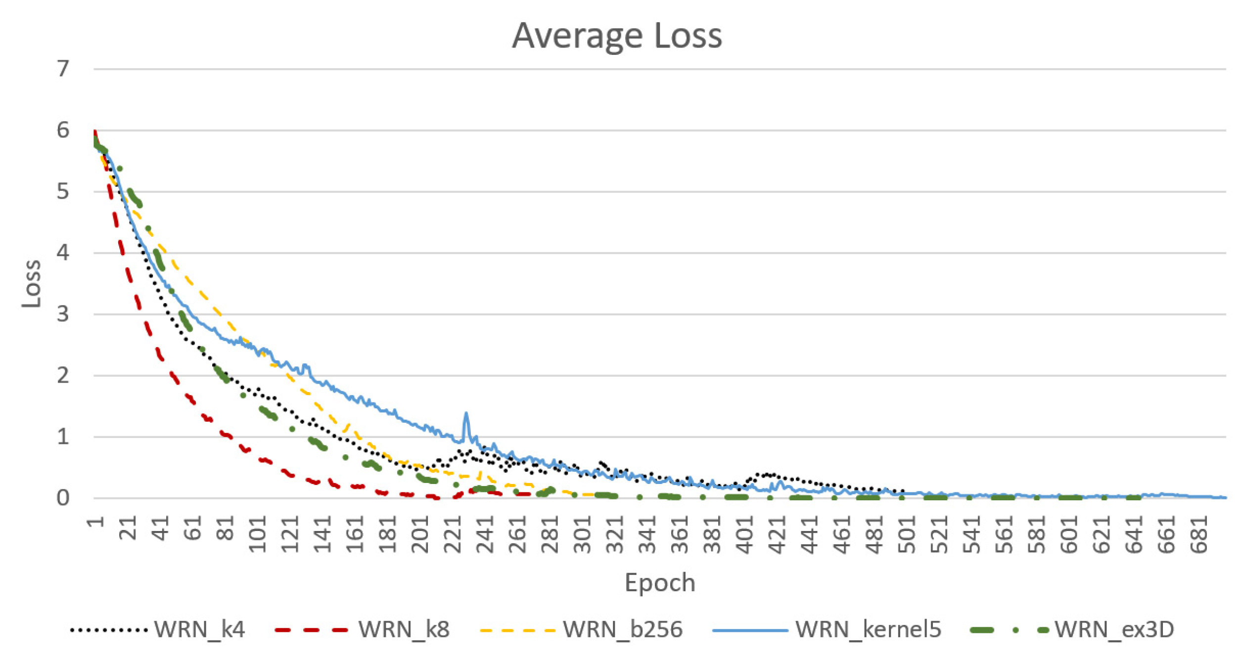
Figure 10 presents the convergence result for average loss under the condition where the samples were randomly distributed between the training and testing sets at a 7:3 ratio. According to Figure 10, the WRN_k8 model, which increased the width of the entire network, effectively reduced the number of epochs required for initial convergence. However, as the model size expanded and the number of parameters doubled, the required time increased by a factor of at least two. Additionally, model WRN_b256, which applied a batch size of 256, reached a similarly low loss with approximately 320 epochs, and thus was quicker than model WRN_k8. Generally, systems with larger batch sizes are more stable and exhibit greater accuracy during testing. However, model WRN_kernel5, in which the size of some kernels was expanded, was less stable than the original model WRN_k4.

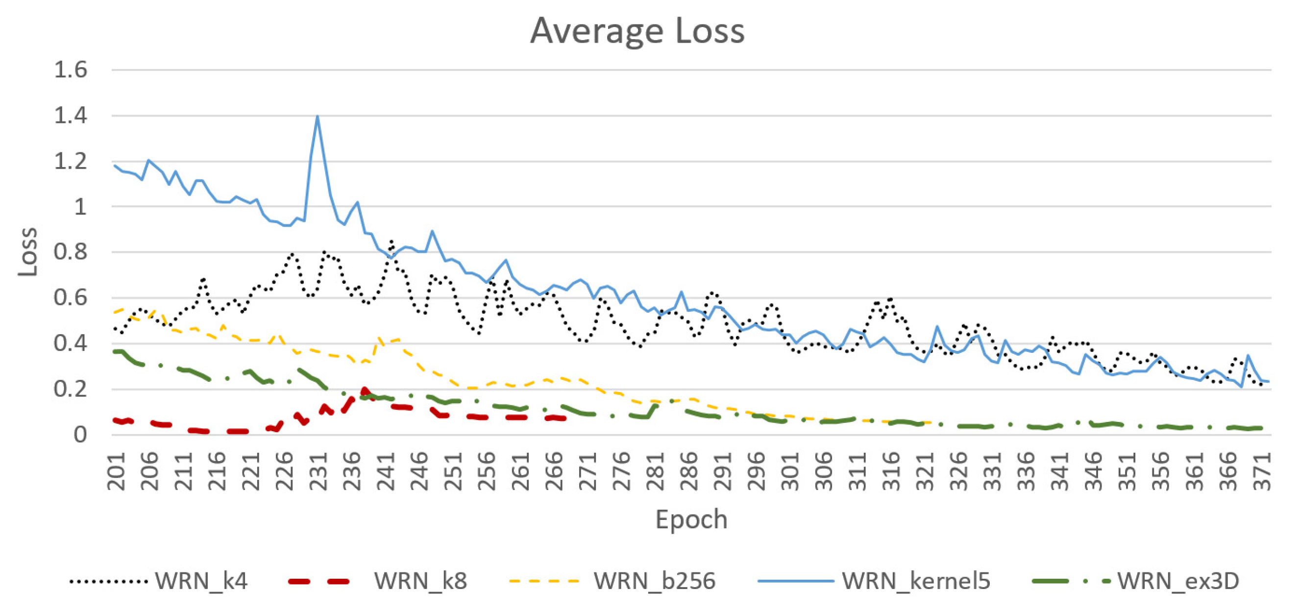
As shown in Figure 11, the WRN_ex3D model which employed the integrated structure of 3D convolution, exhibited stable convergence with approximately the same number of epochs as model WRN_b256 for convergence. In other words, this model required fewer parameters and was relatively quick. Moreover, the limit of loss convergence was low.

7.3.2. Comparison of Loss and Accuracy in The Testing Stage

Because the parameters in the training stage varied according to batch size, the average loss calculated in the training stage was not completely reflected in the testing stage. Therefore, NN performance could not be determined until the testing stage. In addition, the data obtained in the testing stage and training stage differed.

Table 7. Testing results under the condition where the samples were randomly distributed between training and testing sets at a 7:3 ratio.

	Network	Loss	Accuracy
Training Set	WRN_k4	1.667588	66.7036%
	WRN_k8	1.326531	66.7562%
	WRN_b256	0.738129	91.3373%
	WRN_kernel5	0.363532	88.5657%
	WRN_ex3D	0.224468	93.8139%
Testing Set	WRN_k4	1.870392	58.6575%
	WRN_k8	1.554162	59.6236%
	WRN_b256	0.963743	82.5471%
	WRN_kernel5	0.783152	78.2560%
	WRN_ex3D	0.304827	90.3513%

presents the data obtained in the testing stage.

According to Table 7, expanding the network width such as in model WRN_k8 did not increase the representation in this experiment. Longer training might result in a more favorable outcome; however, this approach was inefficient. Moreover, the results of model WRN_b256 revealed sufficient representation with the parameters set at N = 2 and k = 4. The following experiments revealed that with sufficient training time, the model with a batch size of 128 could have similar performance to one with a batch size of 256. This observation verified that a larger batch size benefited the stability of the system.

With respect to the experiment results of model WRN_b256, which was excellent in terms of NN performance, the results obtained from the testing set were notably different from those obtained from the training set. Two possible reasons for this outcome were overfitting and the need to improve the representation of the features that the NN had learned from the training set. Because numerous anti-overfitting methods were employed, such as batch normalization and dropout, the second possibility was more likely to be true. Therefore, this study intended to improve the NN structure to increase the number of features learned.

After referencing [4], the present study incorporated partial 3D convolution layers to extract local temporal features and obtained model WRN_ex3D. The results revealed that this approach effectively improved the convergence rate and reduced the difference between the training and testing set results, with only 864 additional parameters required. Although further computation and more graphics card memory were required to store matrices generated by 3D convolution, this model was more efficient than the other models.

7.4. Dataset Splitting at a 5:5 Ratio

The main objective of this section was to determine which NN could achieve ultimate performance with the highest efficiency. Additionally, model WRN_ex3D was modified. All samples were randomly and equally divided into training samples and testing samples. The NN was trained until extreme convergence was reached. In this experiment, a learning rate of 1 × 10⁻⁴ was employed up to approximately 400 epochs. Slight tuning of the learning rate in accordance with the condition of each model was conducted at the terminal stage of NN convergence to achieve optimal performance. The numbers of samples in the training and testing sample sets were 13,558 and 13,390, respectively.

7.4.1. Convergence Results

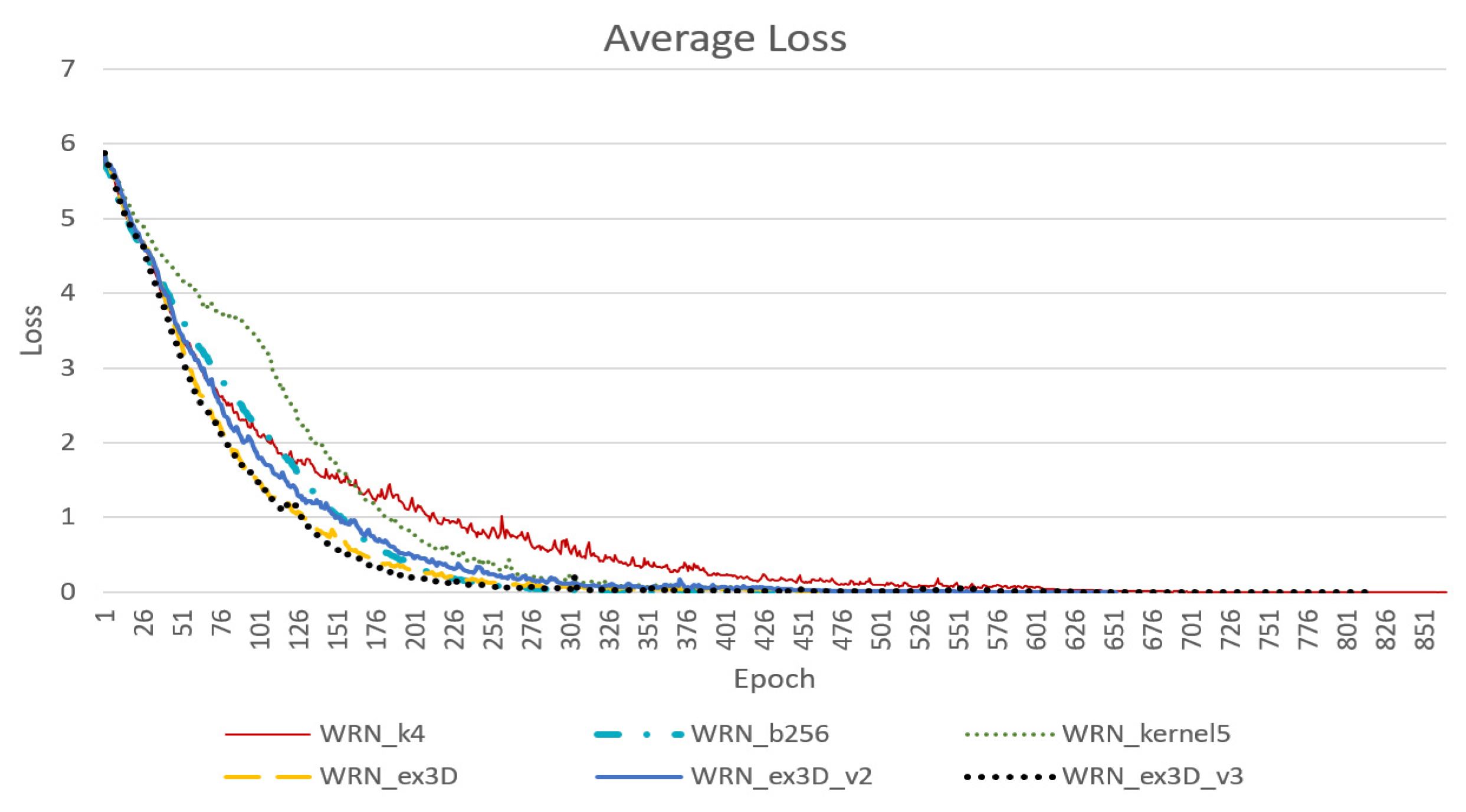
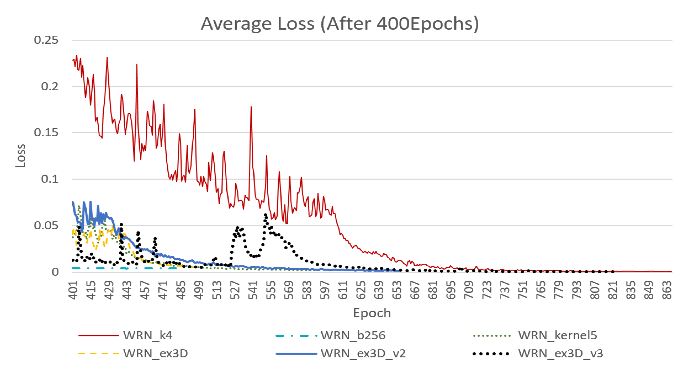
Figure 12 reveals that a larger batch size was beneficial to the convergence rate and system stability, whereas enlarging some kernels hindered NN stability. In addition, networks concatenated with a 3D structure were faster and more stable in terms of convergence. However, among the networks concatenated with a 3D structure, the model that did not remove the original first layer of the 2D convolution layer (WRN_ex3D) was faster in terms of convergence than was the model that removed the 2D convolution layer and widened the channel (WRN_ex3D_v2). Moreover, the model that replaced the mean compression method with a convolution layer with learnable parameters (WRN_ex3D_v3) was even more stable, and the convergence rate was faster than that of model WRN_ex3D.

As shown in Figure 13, enlarging the batch size could stabilize the model. However, ultimate loss stopped at approximately 0.0043 and was unable to be lowered further, even if the learning rate was lowered. In addition, employing a batch size of 128 resulted in instability in the terminal stage; however, ultimate loss reached approximately 0.001, whereas that of model WRN_kernel5 was approximately 0.0026.

With respect to the 3D convolution layer concatenation structure, the original WRN_ex3D model was the most stable and its loss reached the lowest at approximately 0.006. Although model WRN_ex3D_v2 was slow, it was stable in the terminal stage, with an ultimate loss at 0.0014. However, the loss of model WRN_ex3D_v3, which had a 3D convolution layer with learnable parameters, was prone to a sudden rise in the terminal stage. Because of this instability, a less inclined curve for reducing the learning rate was required. The ultimate loss achieved was approximately 0.000448.

7.4.2. Comparison of Loss and Accuracy in the Testing Stage

According to

Table 8. Testing results under the condition where the samples were randomly distributed between training and testing sets at a 5:5 Ratio.

	Network	Loss	Accuracy
Training Set	WRN_k4	0.01442	99.6091%
	WRN_b256	0.01703	99.7418%
	WRN_kernel5	0.123924	96.4154%
	WRN_ex3D	0.017713	99.4837%
	WRN_ex3D_v2	0.013119	99.6755%
	WRN_ex3D_v3	0.004656	99.8746%
Testing Set	WRN_k4	0.268009	93.0769%
	WRN_b256	0.301332	91.6729%
	WRN_kernel5	0.589504	84.6527%
	WRN_ex3D	0.101426	97.0276%
	WRN_ex3D_v2	0.076275	97.4981%
	WRN_ex3D_v3	0.056063	98.3794%

, under the condition where all samples were randomly and equally divided, the results were highly favorable. Models with original structures, namely WRN_k4 and WRN_b256, achieved excellent performance in the training set, which meant that the features learned covered the entire training set. However, the difference between the training and testing set results discussed in the previous section was still observed. In addition, the instability of the system caused by the enlargement of some kernels impeded a notable outcome. Consequently, more epochs were required to reduce the loss in training to an ideal level.

The NN with 3D structure concatenation was not only rapid in terms of convergence during training but also stable. The results of this experiment for the training and testing sets were considerably close. In other words, the 3D concatenation network proposed in this study was capable of improving the overall NN performance, and stabilizing and accelerating model convergence.

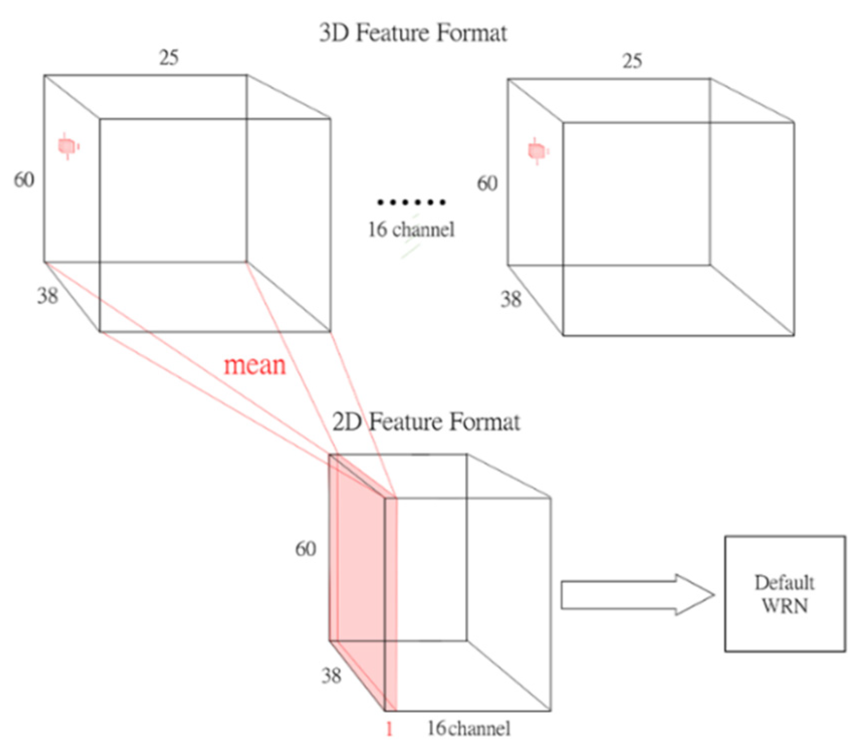
In the meantime, comparing the results of models WRN_ex3D and WRN_ex3D_v2 revealed that the original 2D convolution layer in the first layer became obsolete after the addition of a 3D structure. Additionally, model WRN_ex3D_v3 was a modification of model WRN_ex3D_v2, indicating that using the compression method with learnable parameters to reduce the depth axis (i.e., the time axis) to one dimension was more effective in bringing out the surplus performance of the NN than simply using the mean method to reduce the number of dimensions.

7.5. Effects of Sample Frame Number

The aforementioned experiments revealed that the model established in this study was effective in processing the pedestrian gait optical flow sequence. In particular, samples employed in these experiments were set at 25 frames per unit for training because on average, the pedestrian gait cycle was shorter than 1 s and the average gait cycle from the samples in the sample set was contained within approximately 25 frames. However, the walking speed of each sequence differed. Therefore, another objective of this study was to determine whether accuracy was hindered and enhanced when the sample contained fewer and more than one complete gait cycle, respectively.

In this experiment, the same sample distribution method as that described in D was employed. However, because the distribution was random, the exact training set and testing set differed from those described in D. As shown in

Table 9. Effects of sample frame number on accuracy.

	Sample Frame	Loss	Accuracy
Training Set	15 frames	0.050401	98.40%
	25 frames	0.002754	99.97%
	30 frames	0.000066	100%
Testing Set	15 frames	0.893275	78.35%
	25 frames	0.484642	88.06%
	30 frames	0.341710	92.26%

, the sample was set as having 15, 25, and 30 frames. For fairness, the same sequence of the training set and testing set was applied to the three conditions of frame numbers. The NN employed was model WRN_ex3d because its computational demand was lower than that of model WRN_ex3d_v2 and it was more accurate than the basic model and more stable than model WRN_ex3d_v3. Therefore, the results of model WRN_ex3d were more favorable.

The results revealed that a low sampling frame number hindered accuracy, whereas a high sampling frame number evidently enhanced accuracy. This finding may have resulted from more feature data being contained in a single sample when the sampling frame number was higher. However, increasing the sampling frame number to enhance accuracy raised the computational demand and required more memory. This situation was particularly evident in the model that employed 3D convolution computation.

7.6. Comparison with Related Research

According to Table 10, the dataset employed in studies [5,7] (CASIA) differed from and was much smaller than that employed in the present study, namely the TUM-GAID Gait Dataset. In [5], additional computer-generated data (Human3.6M dataset for foreground and CASIA for background) were employed to increase the data size; however, this takes the model away from reality. In [6], an accelerometer was employed, and in [5,6,7], feature vectors related to displacement were employed as input instead of optical flow. These observations can explain the low reference value of these studies for the present study. Therefore, these studies are not discussed further.

In the method employed in [9], sampling was set at 25 frames per unit. The samples of half of the pedestrians were used for training and those of the other half were tested using transfer learning to verify the effectiveness of the NN in terms of processing gait optical flow. However, this study employed a VGG-like network that contained two fully connected layers and a high number of parameters. Therefore, in addition to a considerable model size, the computational demand was higher than that of the ResNet-based NN model used in the present study. The requirement for equipment was high ([9] used Tesla K40c for experimentation). In addition, the processing method employed in [9] did not conduct tracking on pedestrians in addition to capturing optical flow. By contrast, the present study took the middle segment of the pedestrian image sequences to present the target pedestrian completely in the center of the image and reduced the image size to one-eighth of the original size. However, the method employed in the present study applied automatic pedestrian detection, which focused on the pedestrian, to reduce the number of parameters in the model with a smaller input. In addition, this method had slightly higher accuracy and its data were easier to transfer to other datasets for computation.

Table 10. Comparisons with related research.

Method	Dataset	Accuracy	Parameter Number
[5]	Generated from Human 3.6M dataset & CASIA	83.8%	Over 1.2 million
[6]	iGAIT	98.0%	Over 160 million
[7]	CASIA (Silhouettes)	99.0%	Unspecified
[9]	TUM-GAID(RGB)	98.0%	VGG-based Over 20 million
[8]	TUM-GAID(RGB)	99.78%	WRN (k = 4, N = 3) Approximately 4.285 million
Ours	TUM-GAID(RGB)	98.38%	WRN_ex3D_v3 Approximately 3.173 million

Table 10. Comparisons with related research.

Method	Dataset	Accuracy	Parameter Number
[5]	Generated from Human 3.6M dataset & CASIA	83.8%	Over 1.2 million
[6]	iGAIT	98.0%	Over 160 million
[7]	CASIA (Silhouettes)	99.0%	Unspecified
[9]	TUM-GAID(RGB)	98.0%	VGG-based Over 20 million
[8]	TUM-GAID(RGB)	99.78%	WRN (k = 4, N = 3) Approximately 4.285 million
Ours	TUM-GAID(RGB)	98.38%	WRN_ex3D_v3 Approximately 3.173 million

In [8], Wide ResNet (N = 3, k = 4), which conducted pedestrian detection and pedestrian segmentation, was employed. This method segmented a human body into five parts, namely the entire body, left foot, right foot, upper body, and lower body, and reduced the image size of each part to 48 × 48. Feature vectors extracted from all five parts were then incorporated for NN training. The pedestrian detection method employed in [8] was a simple background-filtering method that was less friendly with data that were unable to provide information of background areas without pedestrians. By contrast, the present study employed YOLOv2 for pedestrian detection. This method was not concerned with the background and extracted the ROI in a rectangular shape fit for the body form of a pedestrian, and thus was capable of filtering excessive background information. Additionally, the preprocessing measure in [8] was more complex than that in the present study because an entire sequence was employed for each sample (the maximum was 90 frames; employment of only 50 frames reduced the accuracy rate to 94.28%). In addition, the optical flow employed was an RGB image (three channels) and the total input size was 48 × 48 × 270. By contrast, the input size of the present study was 60 × 38 × 2 × 25. Therefore, the number of parameters was reduced by more than 1 million. The sampling method was the stepping sliding method. As indicated in Section 4, the method employed in the present study did not require the entire sequence but rather only one or two pedestrian gait cycles for effective recognition.

In summary, the model and preprocessing approach proposed in the present study are more easily adaptable to other input situations compared with those in [9]. The present study conducted far simpler preprocessing than did [8] and applied a superior pedestrian detection method to eliminate excessive input. Moreover, fewer parameters were used in the present study than in [8,9]. Finally, the present study modified the original WRN and developed a 3D-2D concatenated network with enhanced representation that could be applied to solve similar temporal problems.

The accuracy rate obtained by applying multiple data segmentation methods to the same dataset revealed several findings. Regarding the method employed in the present study, the objective was to modify the original WRN model and verify the possibility of improving NN performance for solving gait recognition problems concerning time series. Therefore, the method employed in the present study differed from that employed in [8,9] in that the proposed method used half of all the pedestrians for NN training and the other half for transfer learning to verify the effectiveness of descriptors. Because of these differences, the comparison of accuracy rates detailed in Table 10 merely served as a reference rather than for comparing the efficiency of the different methods.

8. Conclusions

This study employed optical flow to conduct automatic pedestrian detection and recognition. Regarding image preprocessing, automatic pedestrian location detection and pedestrian region extraction techniques were introduced to reduce the size of the optical flow that required processing. Moreover, the method employed in this study could effectively conduct feature extraction while focusing on pedestrian activity to achieve flexible concatenation with other components and facilitate the practical solution and adjustment for similar temporal problems.

The main contribution of this study was determining the possibility of improving the performance of the NN structure for solving temporal gait recognition problems. An additional 3D convolution layer concatenated to the original 2D convolution NN was introduced to conduct dimension reduction along the depth axis (i.e., the time axis). This technique compressed the 3D feature map into a 2D feature map and enabled the original 2D convolution NN to process simplified 3D convolution features. This structure effectively improved NN performance in the face of limited graphics card memory; thus, optimal representation in temporal gait recognition problems and acceleration of the NN convergence rate were achieved. Finally, this study incorporated an additional convolution layer with learnable parameters to replace the original method of obtaining the mean value and enhanced the overall performance of the NN. The 3D–2D concatenated structure established in the present study could be applied to other recognition tasks involving temporal information such as activity recognition and sign language recognition etc.