1. Introduction
This study aims to develop a method for multivariate spatial overdispersion count data. In general, count data can be analyzed using Poisson regression models. However, the assumption of equidispersion in Poisson regression is difficult to fulfill. On the other hand, variance that exceeds the mean (overdispersion) is frequently found when analyzing real data [
1,
2]. Therefore, alternative methods are needed to model data with overdispersion conditions. Mixed Poisson models are often used as an alternative to Poisson regression models, such as the negative binomial (NBR) regression model [
3,
4,
5] and Poisson-inverse Gaussian regression (PIGR) model [
6,
7,
8]. In this study, the PIGR model was chosen because this model performs better when modeling data with high overdispersion. In this study, the PIGR model was developed into a multivariate model with two or more response variables [
9,
10].
The PIGR model is a global regression model that assumes each observation location is influenced by the same predictor. However, in some cases, effects of location cannot be ignored because each location has different characteristics, such as geography and culture, among others. Other spatial regression models, specifically a point-based spatial regression model for overdispersed count data, have been studied. The Geographically Weighted Bivariate Generalized Poisson Regression (GWBGPR) model was used by [
11] to analyze the factors affecting the amount of infant and maternal mortality in East Java, Indonesia. Parameter estimation and hypothesis testing of the Geographically Weighted Multivariate Generalized Poisson Regression (GWMGPR) model has been studied by [
12], theoretically. Both studies use the maximum likelihood estimation (MLE) method and Newton-Raphson (NR) iterative algorithm to estimate the model parameters. The NR methods require the second derivatives of the log-likelihood function with respect to each parameter in the model.
Generalized Poisson regression deals with problem related to over- or underdispersion. Meanwhile, the negative binomial regression (NBR) and PIGR models only deal with overdispersion. The Geographically Weighted Negative Binomial Regression (GWNBR) model was studied by [
13], who applied it to simulation data and real data to show the superiority of the model compared to global regression models, such as the Poisson and negative binomial regression models. The iteratively reweighted least squares (IRLS) and NR methods are often used in parameter estimation. The GWNBR model was also used by [
14] to model the confirmed COVID-19 cases in East Java. The model uses the adaptive bisquare Kernel weighting function and the parameter estimation is performed using a combination of the IRLS and NR methods. The results showed that COVID-19 spread quickly in locations with a high population density. The authors of [
15] evaluated the Geographically Weighted Multivariate Negative Binomial Regression (GWMNBR) in a multivariate way, and the parameters were estimated by combination of the MLE and NR methods. The results showed that the GWMNBR method performed better than the global method.
As mentioned before, the PIGR method only deals with overdispersion, and according to [
1] and other previous empirical studies [
7,
8,
16], the PIGR model has larger variance than the NBR model. Therefore, the PIGR model can accommodate greater overdispersion than the NBR model can. The PIGR model has been developed into a multivariate model with two or more response variables [
10,
17]. Globally, the bivariate Poisson inverse Gaussian regression (BPIGR) model was developed by [
9], while the multivariate Poisson inverse Gaussian regression (MPIGR) was developed by [
10,
18]. Locally, the Geographically Weighted Poisson Inverse Gaussian Regression (GWPIGR) model was created by [
19]. For bivariate cases, Ref. [
20] developed the Geographically Weighted Bivariate Poisson Inverse Gaussian Regression (GWBPIGR) model. To accommodate a combination of global and local parameter estimates, Ref. [
21] developed an alternative GWBPIGR model, namely the Mixed Geographically Weighted Bivariate Poisson Inverse Gaussian Regression (MGWBPIGR) model. In all those studies, parameter estimation was carried out using the MLE and NR methods and the spatial kernel weighting function.
The purpose of this study was to develop a spatial based-point model for multivariate count data with PIG distribution, namely the Geographically Weighted Multivariate Poisson Inverse Gaussian Regression (GWMPIGR) model. The proposed model was developed based on the MPIGR model, which was developed by [
10]. There are two main differences in the model that we developed in this study compared to those that have been developed in previous studies. First, by considering the probability of each occurrence in each research unit, several exposures were used for the case study in this study. We have previously studied univariance, via case study, using the PIGR model with exposure, which performed better than the PIGR model without exposure [
9]. Second, we used the iterative Berndt-Hall-Hall-Hausman (BHHH) methods for parameter estimation. Compared to the NR method, the BHHH method does not need the second derivative of the log-likelihood function with respect to each parameter in the model. This second derivative has the potential to cause problems such as the Hessian matrix and may not be positively definite. It also typically results in a complex nonlinear function that needs to be solved, meaning that the expected value remains unknown. Therefore, the second derivative was eliminated, and a simpler computation with guaranteed convergence was obtained, the BHHH method [
22,
23].
For the real-world application of the proposed model, we analyzed one of the health problems in Indonesia, namely the high number of infant, under-5 and maternal deaths. Numerous studies have been conducted to produce effective policies to reduce the mortality rate of the three groups of individuals. This problem is also one of the targets in the third goal of the SDGs for 2030, living a healthy and prosperous life, which can partially be achieved by reducing the neonatal mortality rate to 12 per 1000 live births and the under-5 mortality rate by 25 per 1000 children under five in the middle of the same year. Furthermore, the maternal mortality rate should also be reduced to less than 70 per 100,000 live births.
Indonesia, the fourth most populous country in the world, is struggling to achieve the 2030 SDG targets for maternal and under-5 mortality. Based on the Indonesian Demographic and Health Survey (IDHS) in 2017, the Maternal Mortality Rate (MMR) was 305 per 100,000 live births. In 2020, the Infant Mortality Rate (IMR) in Indonesia was 17.6 per 1000 live births and the under-5 Mortality Rate (U5MR) was 23 per 1000 live births [
24,
25]. East Java is one of the cities in Indonesia with the highest number of infant, under-5 and maternal deaths compared to other regions in Indonesia. Therefore, it is necessary to study the causal factors to reduce infant, under-5 and maternal mortality in East Java.
In terms of the factors that affect infant, under-5 and maternal mortality, various aspects of life such as socioeconomic status, health facilities, environment, education and culture play equally important roles. Several factors are often the closest factor or the direct cause of the death. These factors include maternal factors, nutrition and disease control in infant and children under five, while bleeding and hypertension are the main causes of death in mothers [
26,
27]. In 2018, Ref. [
28] conducted a study on the factors of neonatal mortality in Indonesia and found that low birth weight (LBW), giving birth to children too close together, medical personnel and postnatal/postpartum visits have a significant effect on neonatal mortality in Indonesia.
In this study, we use four GWMPIGR models, the exposure variable and the spatial weighting function. This study aims to compare on the performance of each model in modeling the number of infant, under-5 and maternal deaths and determine the factors that cause those events based on the best model. District/city level data with different characteristics (spatial heterogeneity) are used. Thus, the form of functions and parameters between locations are divergent. As a result, the parameter significance is also different for each location. Through the GWMPIGR model, districts/cities in Java can be grouped based on predictor variables that significantly affect the number of infant, under-5 and maternal deaths. This grouping is expected to help the relevant agencies make policies to solve this issue.
The specifications of the GWMPIGR model are described in
Section 2, the real-world application of the GWMPIGR model is described in
Section 3 and a discussion of the factors affecting the number of infant, under-5 and maternal deaths in East Java in 2019 based on the selected model will be discussed in
Section 4.
2. Specifications of Geographically Weighted Multivariate Poisson Inverse Gaussian Regression
The MPIGR model is a model that was expanded from the PIGR model, which is a GLMs model with a logarithmic link function. Let (
Y1,
Y2, …,
Ym) ~ MPIG (
μ1, μ2, …,
μm), and the joint probability mass function is as follows:
with
yj = 0, 1, 2, … and
is the dispersion parameter
,
,
, and
is the third modification of the Bessel function [
8]. The properties of the PIGD can be found in [
29,
30]. The MPIGR model can be described as
where
j = 1, 2, …,
m,
is the predicted mean of the
jth response variable,
is the exposure for the
jth response variable, and
τ is the overdispersion parameter.
is the regression parameter that corresponds to the predictor variable
k, for
k = 1, 2, …,
p [
10,
18].
The GWMPIGR model is based on MPIGR model when it incorporates spatial or location-based aspects into the model. The GWMPIGR model is a point-based spatial model where the regression parameters depend on the geographic location. Therefore, each location has different functions and parameters. The GWMPIGR model for the
jth response variable can be written as follows:
where
refer to the longitude and latitude coordinates of the
ith location,
is a regression parameter vector of the
jth response variable for location
i with the following dimension (
p + 1) × 1.
For the GWMPIGR model, parameter estimation is performed using the maximum likelihood estimation (MLE) method and the Berndt-Hall-Hall-Hausman (BHHH) iteration method. At each observation location (point), parameter estimation is carried out using a spatial weighted matrix (W). The elements of matrix W show how much influence the observations at a particular location have on the surrounding observations (wii*).
The joint probability mass function of
Yi1,
Yi2, …,
Yim with
j = 1, 2, …,
m, i = 1, 2, …,
n and
coordinates is as follows:
with
,
,
,
j = 1, 2, …,
m,
, and
.
Let
is the vector of parameter the GWMPIGR model. Then, the likelihood function for the GWMPIGR model is
Let
is the vector of parameter for location
i*. Then, the likelihood function to estimate the parameter at location
i* with the spatial weighted matrix
wii* is as follows:
The log-likelihood function of Equation (6) is as follows:
Several methods can be used to determine the spatial weights for each different location in the GWMPIGR model, including the kernel function. There are two types of the kernel functions: the fixed kernel function and the adaptive kernel function. The difference between those two functions lies in the bandwidth value (
h). The bandwidth value for the fixed kernel function is the same for every location (
h). Meanwhile, the bandwidth value for the adaptive kernel function is different for every location (
hi). In this study, we used fixed kernel functions, specifically the fixed Gaussian kernel functions and fixed bisquare kernel functions. The fixed Gaussian kernel function is formulated as follows:
Meanwhile, the fixed bisquare kernel function is
with
is the eucliden distance between location
and location
and
h is a smoothing parameter (bandwidth).
The bandwidth value is related to the accuracy of the model. A very small bandwidth value causes the variance to become larger. On the other hand, a large bandwidth value can cause a larger bias. Therefore, it is very important to choose the appropriate bandwidth value. According to [
31], the selection of the optimal bandwidth value can be achieved using the cross validation (CV) criteria, which can be formulated mathematically as follows:
The ML estimator that maximizes the log-likelihood function of the GWMPIGR model in Equation (7) is obtained by solving the system of equations for all of the first partial derivatives of the log-likelihood function for each parameter and then equating it with zero as follows:
The first-order partial derivatives of the log-likelihood function are as follows:
where
The first derivative of the log-likelihood function of the GWMPIGR model parameters (Equations (12)–(15)) is non-closed-form equation. Thus, the estimator value is obtained through the Berndt-Hall-Hall-Hausman (BHHH) iteration method using the following algorithm:
- Step-1
Determine the initial value of each parameter using the results of the MPIGR model parameter estimator.
- Step-2
Define the gradient vector
with the first derivative (Equation (11)) as the element.
- Step-3
Define the Hessian matrix
,
where
is the individual gradient vector.
- Step-4
Define the tolerance limits (ε = 10−3) and maximum iteration (t* = 1000).
- Step-5
Start the BHHH iteration using the following equation:
- Step-6
The iteration will stop at the t* iteration or at the value of
Repeat this algorithm for each location i (i = 1, 2, …, n).
The simultaneous hypothesis testing of the GWMPIGR model parameters is carried out by testing H
0:
versus H
1: at least one
, where
j = 1, 2, …,
m;
k = 1, 2, …,
p; and
i = 1, 2, …,
n. The following statistical test used is:
where
is the log-likelihood function for a parameter set under population
and
is the log-likelihood function for a parameter set under the null hypothesis
.
The log-likelihood function of GWMPIGR model for parameter set under population is:
The log-likelihood function of GWMPIGR model for parameter set under H
0 is:
The estimator value for the parameter set under H0 are obtained using the same steps as those for estimating the parameters of the GWMPIGR model.
The
G2 test statistic (Equation (18)) has a
, where trace(
R) is the number of effective parameters for the GWMPIGR model, in which the elements of the matrix
R are formulated as follows:
The critical area for testing the regression parameter hypothesis can be determined for the GWMPIGR model simultaneously by rejecting H
0 if the value of
[
32,
33].
This study will compare several models based on the exposure variable and the spatial weighting function used. The exposure variable in the GWMPIGR model in Equation (3) can consist of the same or different exposure levels for all of the response variables. Therefore, the best model will be selected using the corrected AIC (AICc) value:
where
k* is the number of effective parameters in the GWMPIGR model, and
is the likelihood function of the GWMPIGR model (Equation (5)).
3. Results
This section shows the fit of the GWMPIGR model on the number of infant, under-5 and maternal deaths in East Java in 2019. The data were sourced from the Public Health Office and Statistics Indonesia. The Health Office of Indonesia provides data on health indicators from the provincial and district/city levels, and these data are published regularly every year. Meanwhile, Statistics Indonesia provides data for all indicators (including health), and these data are published annually. District/city level data are provided by the Public Health Office and Statistics Indonesia for every province in Indonesia.
In this study, the data consisted of 38 districts/cities in the province of East Java Province, and there were three response variables: the number of infant deaths (
Y1), the number of under-5 deaths (
Y2) and the number of maternal deaths (
Y3); five predictor variables: the percentage of active integrated service post (
X1), the percentage of active family planning participants (
X2), the percentage of the population with BPJS health insurance (
X3), education index (
X4) and the percentage of household that has improved sanitation (
X5); and three exposure variables sourced from the Public Health Office and Statistics Indonesia. Four models will be used based on the exposure and the spatial weighting function, as presented in
Table 1.
The first two GWMPIGR models only had one exposure variable, the number of live births, which was used by considering the definitions of the mortality rate for each individual group. Meanwhile, the third and fourth models use three exposure variables by considering the number of people who are at risk in each individual group. The best of the four models will be selected based on the AICc value. Then, the factors affecting the number of infant, under-5 and maternal deaths in East Java in 2019 are discussed based on the best model.
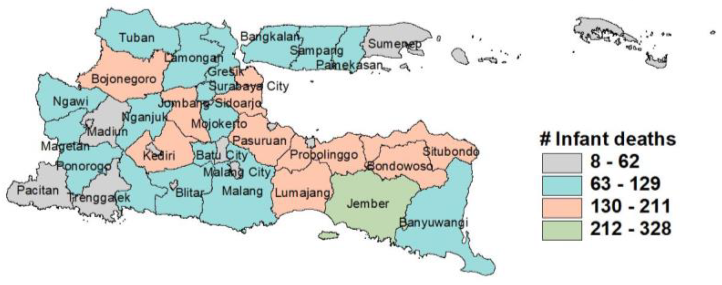
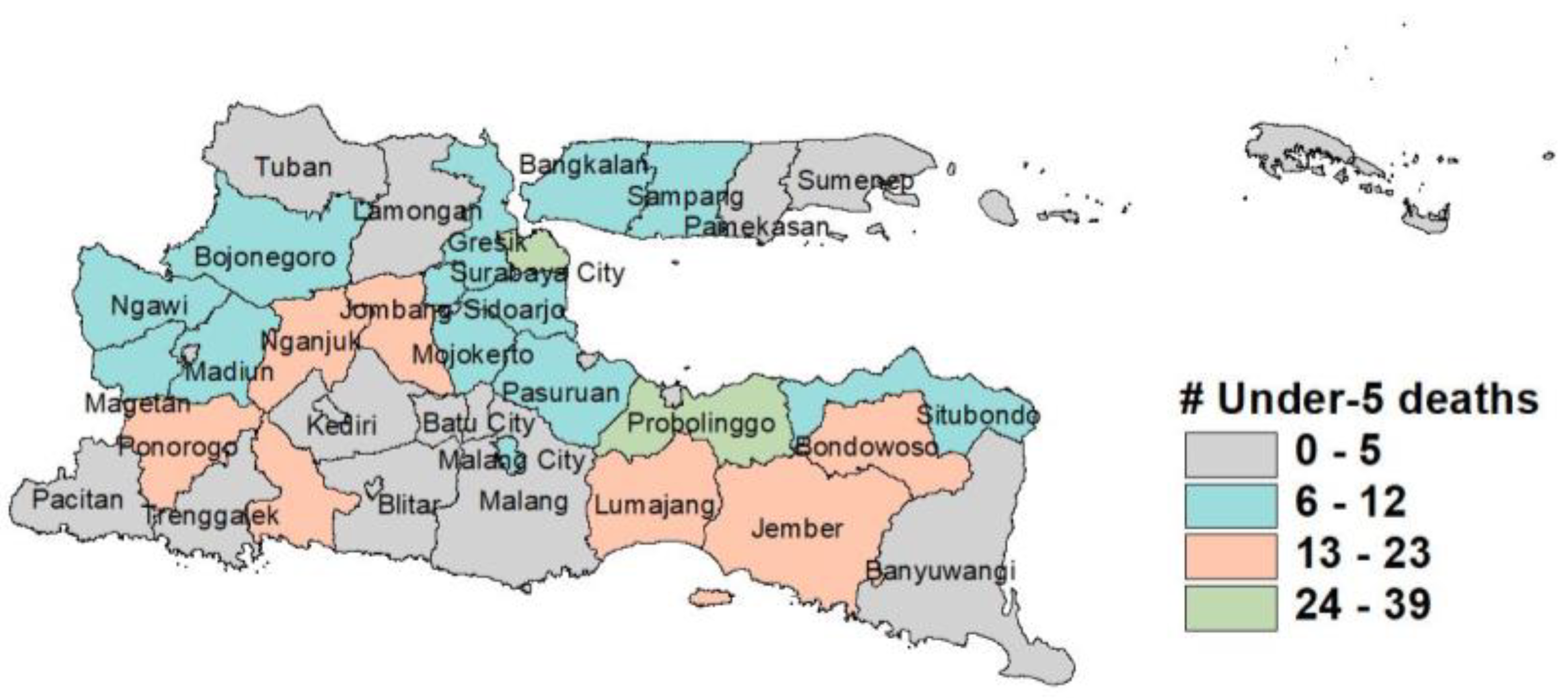
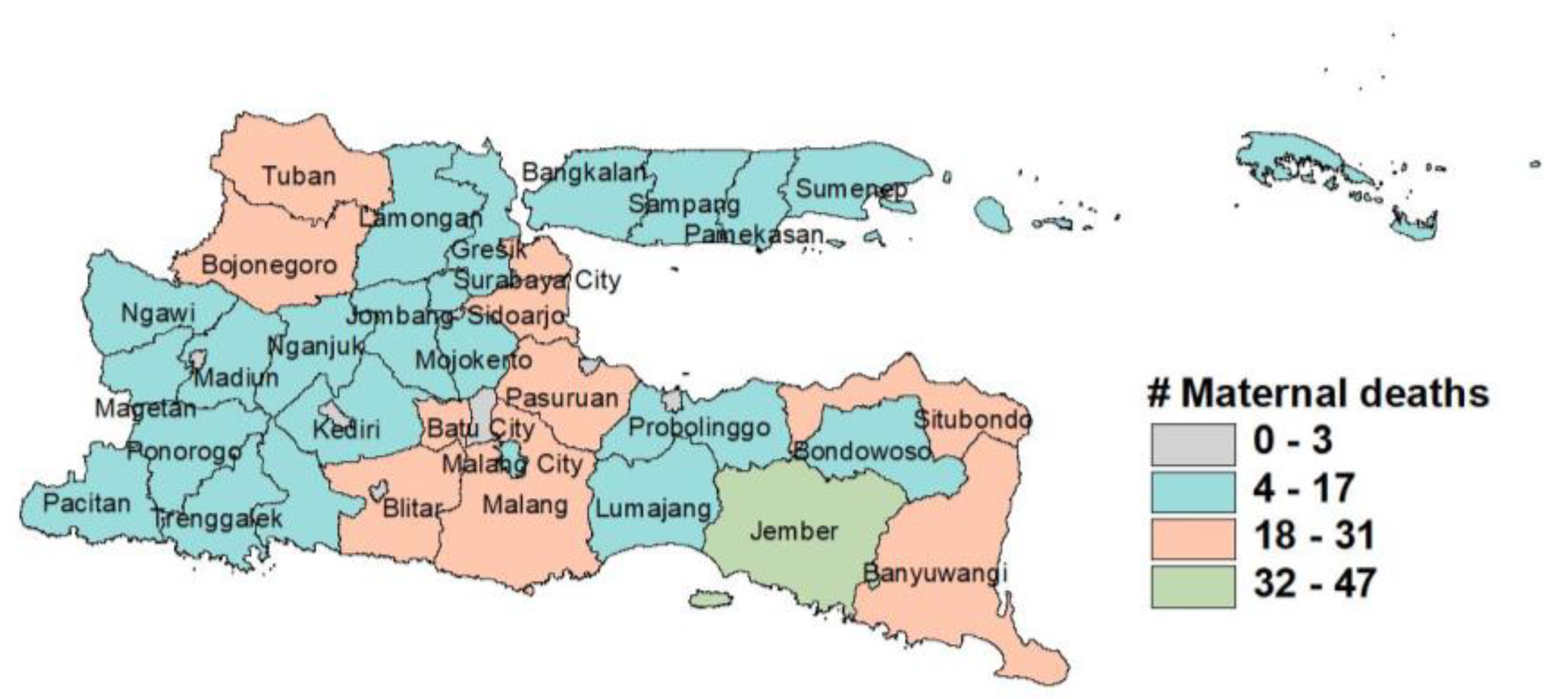
Figure 1,
Figure 2 and
Figure 3 are thematic maps that provide descriptions of the response variables. The number of deaths in each population is divided into four levels from the lowest to the highest number of deaths in the district/city.
Figure 1 and
Figure 3 show that most of the districts/cities in East Java have a high number of infant and maternal deaths. Meanwhile,
Figure 2 shows that the Probolinggo District and Surabaya City have the highest number of under-5 deaths. Furthermore, the summary statistics of the predictor variables and exposure variables can be seen in
Table 2.
According to
Table 2, the mean of the active integrated service post in East Java in 2019 was 80.95%, with a minimum percentage of 31%. Furthermore, the mean of active family planning participants is 75.4%, with a minimum percentage of 67.03%. This means around 33% of people do not participate in family planning. The mean of the population with BPJS health insurance is 50.47%, which means that the other half of population uses other types of health insurances. The mean of the education index is 0.628. The education index is calculated based on the expected years of schooling and the mean years of schooling. The higher the value of the education index, the better the quality of education and society, which will consequently improve the quality of life. As for the environment variables, there was a large gap in the percentage of households with improved sanitation, with the minimum percentage being 25.25%. This means that there are still many households with inadequate sanitation.
Furthermore, a multicollinearity test, which assumes that there is no relationship among predictor variables (mutually independent), was carried out as a requirement for the regression analysis. In this study, the variance inflation factor (VIF) criteria was used to identify multicollinearity among predictor variables. The last column in
Table 2 shows that the VIF value of all of the predictor variables is lower than ten (VIF < 10). Thus, there are no multicollinearity issues among the predictor variables.
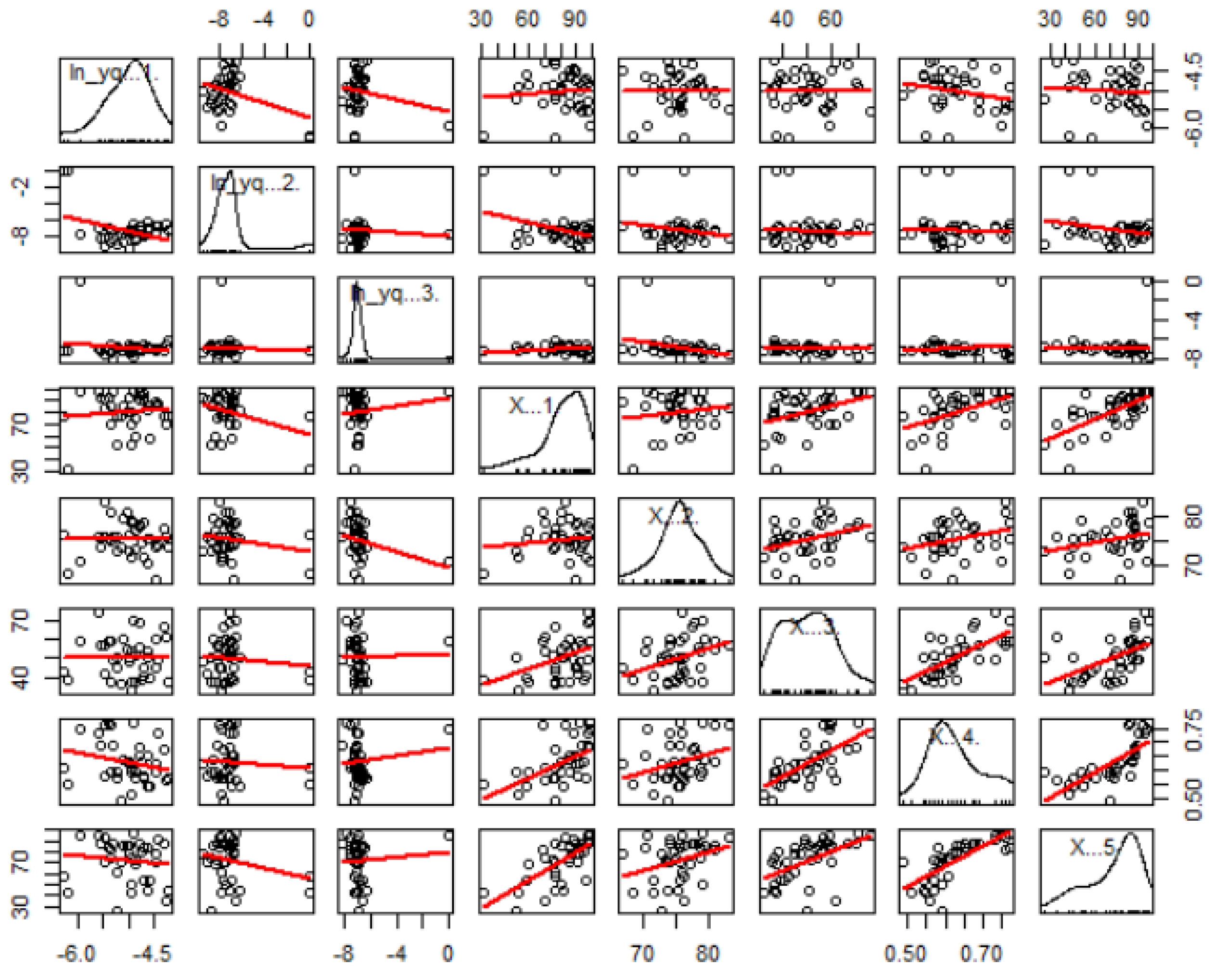
An initial examination of the relationship between the response and the predictor variables is important because it relates to the initial description of the relationships between variables found in the modeling. Based on
Figure 4, the relationship between the predictor variable and the response variable seems non-linear. Log(
Y1/
q1) has the strongest correlation with
X3 (−0.23). Meanwhile, log(
Y2/
q2) has the strongest correlation with
X1 (−0.36) and log(
Y3/
q3) has the strongest correlation with
X2 (−0.29).
Several assumptions must be met before carrying out GWMPIGR modelling. Specifically, the response variable is not Poisson distributed, and there is spatial heterogeneity. Testing the distribution of the response variables was carried out using the Crockett test, and it was found that the response variables did not have a trivariate Poisson distribution (because there were three responses). This result is also supported by the issue of overdispersion on the response variables. The methods used to test the overdispersion are deviance per degree of freedom (deviance/df) and the Lagrange multiplier (LM) test, the test results of which are shown in
Table 2.
Overdispersion exists if the value of deviance/df is greater than one and the LM method produces a value of
or a
p-value of <
α. Based on
Table 3, there are cases of overdispersion on the response variable. Therefore, the GWMPIGR model can be used to model data on the number of infant, under-5 and maternal deaths in East Java in 2019. Furthermore, the spatial heterogeneity test was carried out by using the Glejser test and it was found that there is spatial heterogeneity when the test statistics value
G = 210.5993 is larger than
.
The parameter of the GWMPIGR model were estimated locally using spatial weighting so that each observation location had a different parameter estimate value. Spatial weighting represents the location between observations. The closer an observation location is to another observation location, the greater the weighting value and the greater the influence on these observations. In this study, spatial weighting was determined using a fixed Gaussian and bisquare kernel function. The optimum bandwidth, minimum CV and AICc values for each model are presented in
Table 4.
Based on
Table 4, model 2 has the lowest CV minimum value. However, this does not mean that model 2 is the best model. The CV value is used to determine the optimum bandwidth for the spatial weight matrix. Therefore, the CV values in
Table 4 refer to the minimum CV value of the optimum bandwidth for each model. On the other hand, the AICc can be used to evaluate how well a model fits the data and to determine the best model from multiple models for the same dataset. AICc uses the MLE of the model (log-likelihood) as a measure of fit. The model that fits the data the best has the maximum likelihood. Therefore, the model with high log-likelihood has a low AICc value. Based on
Table 4, model 1 has the smallest AICc value. Thus, in this study, the GWMPIGR model with the fixed Gaussian kernel spatial weighting function and the number of live births as the exposure is the best model to determine the number of infant, under-5 and maternal deaths in East Java in 2019. Therefore, only model 1 will be discussed further.
The value of the parameter estimator of the GWMPIGR model is different for each observation location, as is the significance of the parameters. The GWMPIGR model generated 722 coefficient estimates for 38 districts/cities in the province of East Java. Simultaneous testing of the GWMPIGR model parameters shows that at least one parameter has a significant effect on the response variable (
G2 = 384.17 >
). Meanwhile, partial hypothesis testing was carried out on the parameters of the GWMPIGR model locally for each observation’s location. For example, the parameter estimates for the GWMPGR model with the fixed Gaussian kernel spatial weighted function for Banyuwangi District (
i = 10) and Surabaya City (
i = 37) can be seen in
Table 5.
Table 5 shows that there are differences in the parameter coefficient values and in the parameter significance for Banyuwangi District and Surabaya City. Some of the predictors that were significant in Surabaya City were not significant in Banyuwangi District. Variable
X3 and
X5 did not significantly affect
Y1 in the Banyuwangi District, while all of the predictors significantly affected
Y1 in Surabaya City. Variables
X1,
X3 and
X5 did not significantly affect
Y2 in the Banyuwangi District, while only variable
X3 did not significantly affect
Y2 in Surabaya City. Meanwhile, similar parameter significance was found for the variable
Y3 More specifically, variable
Y3 is equally influenced by variables
X2 and
X4 in the Banyuwangi District and Surabaya City. The significance of the parameters of the GWMPIGR model in other regencies/cities in the province of East Java that are different is that they can then be formed into several regional groups according to the predictors that significantly affect the number of infant, under-5 and maternal deaths. This grouping will be discussed further in the Discussion section.
To provide an example, the GWMPIGR model for Surabaya City based on
Table 5 is presented as follows:
The value of the regression parameter coefficients in the model above shows the magnitude of the change in the average number of infant, under-5 and maternal deaths in Surabaya due to the influence of each predictor variable. The interpretation of the model will be discussed further in the discussion section.
4. Discussion
Model 1’s performance for Surabaya City was interpreted based on each predictor variable. Increasing the percentage of active integrated service posts (X1) will increase the average number of infant deaths (Y1), reduce the average number of under-5 deaths (Y2) and increase the average number of maternal deaths (Y3). However, X1 does not significantly affect the number of maternal deaths (Y3).
Increasing the percentage of active family planning participants (X2) will increase the average number of infant deaths (Y1), reduce the average number of under-5 deaths (Y2) and reduce the average number of maternal deaths (Y3). Increasing the population with BPJS health insurance (X3) will increase the average number of infant deaths (Y1), reduce the average number of under-5 deaths (Y2) and reduce the average number of maternal deaths (Y3). However, X3 does not significantly affect the number of under-5 deaths (Y2) or the number of maternal deaths (Y3).
Increasing in education index (X4) will reduce the average number of infant deaths (Y1), increase the average number of under-5 deaths (Y2) and increase the average number of maternal deaths (Y3). Moreover, increasing the percentage of households with improved sanitation (X5) will reduce the average number of infant deaths (Y1), reduce the average number of under-5 deaths (Y2) and increase the average number of maternal deaths (Y3). However, X5 does not significantly affect the number of maternal deaths (Y3).
Table 6 shows the differences between correlation and GWMPIGR modelling for Surabaya City. Some predictors have a consistent relationship with correlation, and some do not. As we can see that the correlation between the number of under-5 deaths (
Y2) and education index (
X4) or the percentage of household that has improved sanitation (
X5) is not the same as that observed in the GWMPIGR modelling. Additionally, the correlation between the number of under-5 deaths (
Y3) and the percentage of the population with BPJS health insurance (
X3) is not consistent with the GWMPIGR modelling. However,
X3 shows that it is not significantly correlated with
Y3 and that it does not significantly affect
Y3. However, the pattern of the relationship between the response variable and the predictor variable is different for each location.
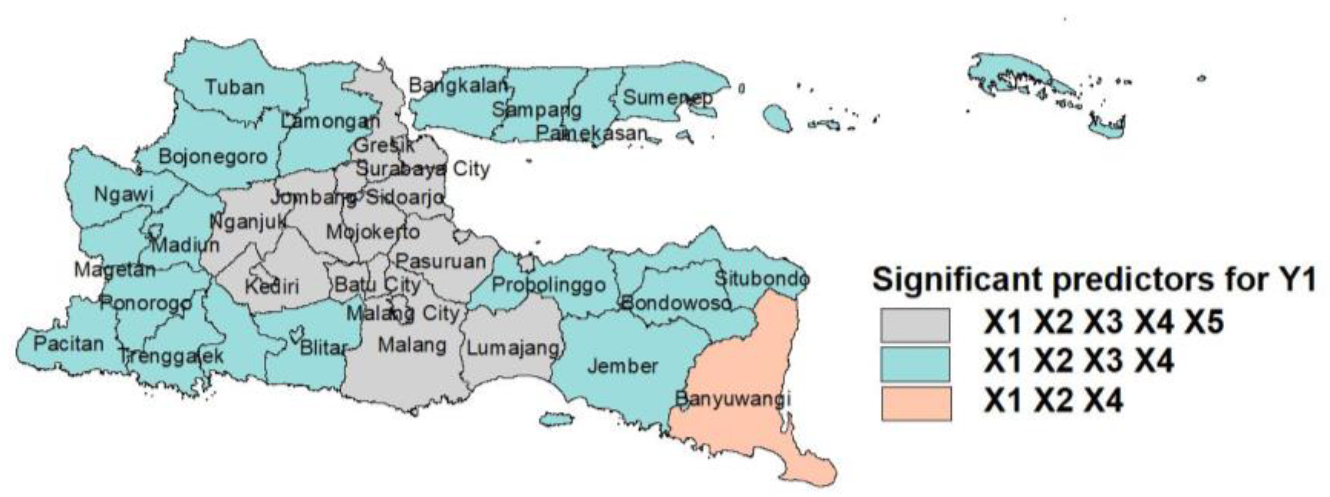
Furthermore, the results of the parameter testing for the GWMPIGR model 1 produced several regional groups based on significant predictors, which are presented in
Table 7.
There are three regional groups according to the significant predictors for the number of infant deaths and the number of under-5 deaths, while there are two regional groups based on significant predictors for the number of maternal deaths. For the number of infant deaths (Y1), 16 districts/cities in East Java are affected by all of the predictor variables, 21 districts/cities are influenced by the percentage of active integrated service post (X1), the percentage of active family planning participants (X2), the percentage of the population with BPJS health insurance (X3), education index (X4) and only one district/city is affected by the percentage of active integrated service post (X1), the percentage of active family planning participants (X2) and education index (X4).
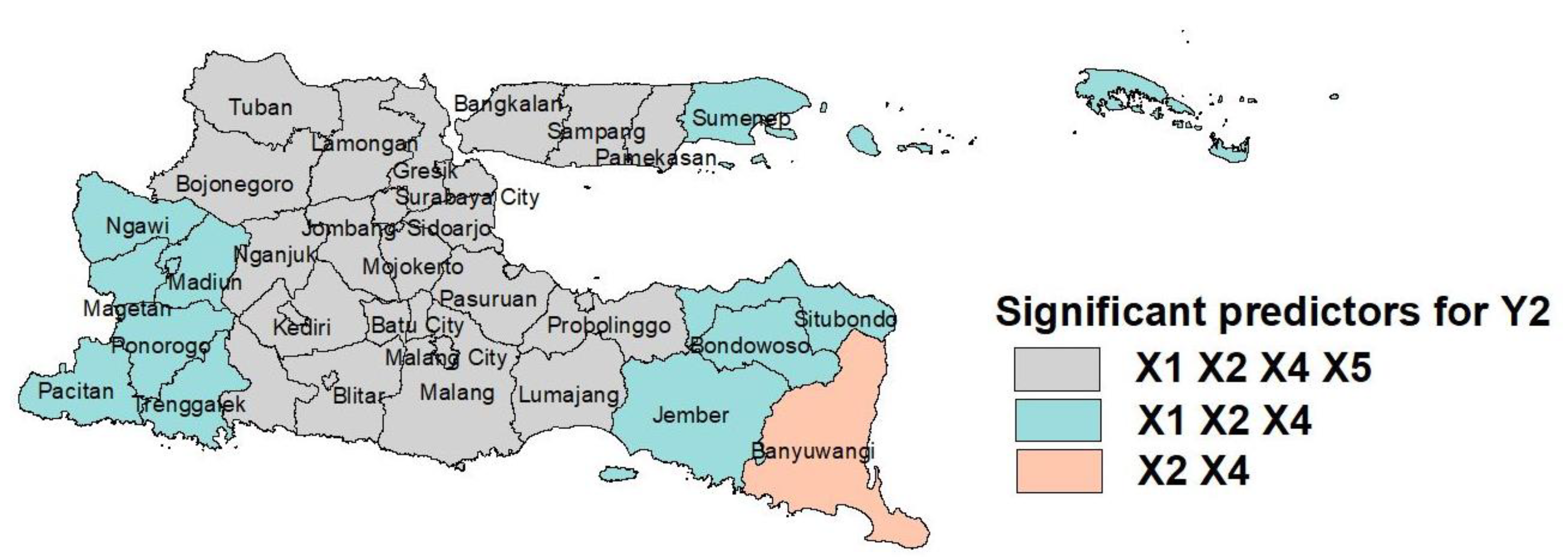
For the number of under-5 deaths (
Y2), 11 districts/cities in East Java are affected by the percentage of active integrated service post (
X1), the percentage of active family planning participants (
X2), education index (
X4) and the percentage of households that have improved sanitation (
X5), 26 districts/cities are influenced by variables the percentage of active integrated service post (
X1), the percentage of active family planning participants (
X2) and education index (
X4) and only one district/city is affected by the percentage of active family planning participants (
X2) and education index (
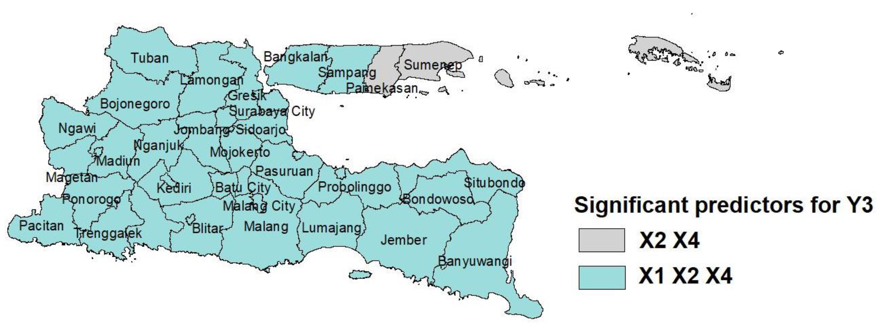
X4). Moreover, for the number of maternal deaths (
Y3), 36 districts/cities in East Java are affected by the percentage of active integrated service post (
X1), the percentage of active family planning participants (
X2) and education index (
X4) and two districts/cities are affected by the variables the percentage of active family planning participants (
X2) and education index (
X4). Visually, the groupings are presented in the thematic maps shown in
Figure 5,
Figure 6 and
Figure 7.
Based on
Figure 5,
Figure 6 and
Figure 7, the GWMPIGR modeling forms several regional groups. Each group is assumed to have the same characteristics, so the predictors that significantly affect each event are also the same. Thus, this will make it easier for the government to make policies to decrease the number of infant, under-5 and maternal deaths. For example, based on
Figure 7, the percentage of active family planning participants and the education index affect the number of maternal deaths in the Pamekasan and Sumenep districts. Therefore, those two districts should focus on increasing the number of people using family planning services and on improving the quality of education. The same applies to other regional groups.


 : The best model.