Dynamic Analysis on the Parametric Resonance of the Tower–Multicable–Beam Coupled System

Abstract

Considering the effect of the bridge deck’s bending stiffness and the indirect effect of adjacent cables (CEB), this paper aims to propose a refined model to reliably analyze the complex internal resonance mechanism of the tower–multicable–beam coupled system (MCS) under nonlinear geometric conditions. To accurately analyze the dynamic behavior, the shear difference effect is applied to simulate the continuous rigidity of the single beam. The dynamic equations of the whole resonance system are derived based on the D’Alembert Principle and the Finite Difference Method, the Galerkin Method and verified by the case study. The results of the numerical simulation based on the Fourth Runge–Kutta Method show that the dynamic parameter of each component is closely related to the coupled resonance of the system. The dynamic behavior under two conditions, tower–cable 1:1 resonance (TCR) or cable–beam 1:2 resonance (CBR), is deeply analyzed. Additionally, the excitation effect of the maximum amplitude by two excitation approaches, the initial displacement or initial velocity, both show a linear increase. The mutual transmission process of vibration excitation on the cable through the bridge beam or the tower as the medium is also further discussed.

1. Introduction

Complex spatial cable architecture, such as long-span cable-stayed bridges, exhibits a complex dynamic characteristic [1]. Due to the periodic change in the lateral restoring force of the cable, the lateral vibration of the cable is coupled with the horizontal/vertical vibration of the tower/beam. When the ratio of the local modal frequency of the cable to the overall modal frequency satisfies a certain relationship, 1:1 or 1:2, a strong and complex coupled internal resonance will occur in the combined structure [2,3,4]. So far, the same characteristic violent vibrations of the cable with a maximum lateral amplitude exceeding 1 m have been observed in real bridge monitoring in many countries [5,6]. The failure of the dampers on the stay cables caused by this severe vibration will further reduce the structural stiffness and also seriously affect the safe operation of the bridge [7].

To address this problem, a number of researchers have carried out a wealth of theoretical and practical research. Kang [8], Song [9] and Cong [10] proposed a number of dynamic models reduced from the cable-stayed bridges according to different research objects and analyzed the parameter sensitivity of the parametric resonance by various numerical simulation methods, such as the Runge–Kutta Method, the Multi-Scale Method and others. Focusing on the different resonance conditions, 1:2 and 2:1, of cable–beams, investigations were conducted to deeply analyze the characteristics of the parametric resonance in cable–beam structures [11]. Gattulli V. [12] investigated the mechanism of resonance change caused by cable end angle changes and analyzed the conversion of low-frequency vibration and high-frequency vibration from the perspective of energy transfer. Wang [13] analyzed the influence factors, such as the frequency ratio of the cable-beam, the excitation amplitude, the cable force and cable dampers, on the characteristics of structural coupling by the numerical simulation of a proposed model. In addition, Sun [14,15] observed the severe vibration phenomena of 2:1 resonance through the model experiment of the cable-stayed bridge and studied the process of mode shape coupling under different order modes. Zhang [16] conducted the resonance interval of the frequency ratio between the cable to beam or tower through a field experiment of the existing bridges. Moreover, Caetano [17] concluded that the linear cable–deck interaction under the first two internal resonance modes was considered to be the key excitation source for the cable oscillation with a large amplitude through the experimental data on Guadiana Bridge. Ouni [18] investigated the structural dynamic instability phenomenon when the local mode and global mode were coupled. The influence of excitation amplitude and additional damping on the steady-state response of stay cables under parametric excitation was further discussed through finite element analysis and field experiments.

It has been concluded that the parametric excitation polynomial in cable vibration differential equations is one of the main factors that cause global–local resonance in the combined systems of cable-supported bridges [12]. It is illustrated that the finite element model requires a large number of subdivisions to perform the fine analysis of the coupled parametric resonance well [19], and it is definitely difficult to analyze the dynamic characteristic of the full-bridge resonance accurately. Thus, limited by the difficulty of accurate finite element division and field testing of bridges, researchers have conducted a number of refined studies focusing on the parameter sensitivity analysis of the dynamic behavior of a single-cable system [20,21,22,23]. However, the vibration of a single cable does affect the vibration characteristics of other cables through the indirect effect transformed by the beam or the tower [24], and the local resonance effect under the single-cable system cannot accurately reflect the resonance effect under the MCS of the cable-stayed bridge. More knowledge should be obtained through further studies on the nonlinear dynamics modeling of the full-bridge system [25].

In this paper, the shear difference in the beam section at each cable’s anchored position is applied to simulate the effect of the bridge deck’s bending stiffness and the indirect effect of adjacent cables (CEB). Considering the parabola alignment of the cable and the boundary of the system, the ordinary differential equations (ODEs) of the vibration system are derived based on the D’Alembert Principle and the Galerkin Method. The case study is adopted to verify the effectiveness of the modeling, while the mode shapes of the single beam obtained by this method and the finite element method are discussed in depth. The effect of the dynamic parameters obtained from the equation forms and that of the excitation sources on the parametric resonance have been further investigated through the numerical simulation based on the Fourth Runge–Kutta method.

2. The Dynamic Model of the MCS

2.1. The Vibration Equations of the Tower and the Cable

The parametric resonance of the cable excited by the tower or the beam is the object of this investigation. To focus on the object, the dynamic model of a tower–six-cables–beam structure is established, as shown in Figure 1A. It is agreed that the relevant parameters of towers, cables, and beams are subscripted by t, c and b; the C1#~C6# cable corresponds to the 1#~6# subsystem, and the reduced model of the Ci# cable is shown in Figure 1B. The nomenclature list for the variable parameters is selected as shown in

Table 1. The nomenclature list for the variable parameters.

Designation		Parameter
Tower	Unit mass	$m_t\left(z\right)$
	Static modulus of elasticity	$E_t$
	Bending moment of inertia	$I_t$
	Damping coefficient	$c_t$
	Height	$L_t$
	Lateral vibration displacement	$v_t\left(z,t\right)$
Ci# cable	Unit mass	$m_{ci}\left(x_{ci}\right)$
	Static modulus of elasticity	$E_{ci}$
	Cross-sectional area	$A_{ci}$
	Static alignment	$w_{ci}\left(x_{ci}\right)$
	Vibration displacement in the chord direction	$u_{ci}\left(x_{ci},t\right)$
	Vibration displacement in the transverse direction	$v_{ci}\left(x_{ci},t\right)$
	Static tension in the chord direction	$H_{ci}$
	Dynamic tension in the chord direction	$h_{ci}$
	Static tension in the tangential direction	$T_{ci}$
	Dynamic tension in the tangential direction	${\tau }_{ci}$
	Displacement of the cable in chord direction	$L_i$
	The length of the cable under the static state	$L_{ci}$
	Sag of the Ci# cable at the midspan position	$D_{ci}$
	Damping coefficient	$c_{ci}$
	The angle of the cable with beam	${\theta }_i$
Bi# beam portion	Mass	$M_{bi}$
	Static modulus of elasticity	$E_{bi}$
	Bending moment of inertia	$I_{bi}$
	Damping coefficient	$c_{bi}$
The generalized coordinates, limited with time		$V_t\left(t\right)$$, V_{ci}\left(t\right)$$, V_{bi}\left(t\right)$
Acceleration of gravity		g

.

In Figure 1B, the directions of $x_{ci}$ and $y_{ci}$ represents the chord and transverse direction of the cable vibration, respectively. To highlight the research emphasis, some assumptions are given as follows [15,21]: (i) the influence of cable bending and torsion stiffness on vibration is negligible; (ii) the influence of the cable’s gravity on the string tension in the chord direction is ignorable; (iii) the flexural, torsional, shear strain and the longitudinal inertia force of cables are ignorable; (iv) it is believed that the deformation constitutive relationship of the cable and the bridge tower satisfies Hooke’s law when it vibrates; and (v) the axial influence of stay cable on the tower and the beam segment is ignorable.

In Figure 1, the bridge tower can be regarded as a cantilevered tower with a rigid foundation, cast-in boundary condition and upper-end tension without considering the influence of foundation deformation or the superstructure. It is noticeable that this paper aims to propose a refined model for investigating the simulation of the CEB on the parametric resonance of the whole dynamic system. On this basis, it is assumed that the cables are anchored at the same position of the tower. It is easy to obtain the partial differential equations (PDEs) of the tower as follows:

$$M_t^{*}·{\ddot{v}}_t\left(z,t\right)+{\dot{c}}_t·{\dot{v}}_t \left(z,t\right)+K_t^{*}·v_t\left(z,t\right)=F_t^{*}$$

(1)

where $M_t^{*}$, $K_t^{*}$ and $F_t^{*}$ represent the equivalent mass, equivalent stiffness and equivalent external force, respectively, and the detailed derivation process is shown in Appendix A. The in-plane lateral vibration displacement of the tower is as shown in Equation (2):

$$v_t\left(z,t\right)=\sum _{n=1}^n{\phi }_{tn}\left(z\right)·V_t\left(t\right)$$

(2)

where ${\phi }_{tn}\left(z\right)$ represents the mode shape of the nth-order. To reduce the amount of calculation, the following research only studies the first order of the mode shape (n = 1, ${\phi }_t\left(t\right)={\phi }_{t1}\left(t\right)$). The boundary conditions of the tower are:

$$v_t\left(0,t\right)=0, v_t\left(L_t,t\right)=V_t\left(t\right)$$

(3)

To avoid complex calculations, only the first mode shape of the tower which satisfies the geometry and the dynamic boundary conditions is selected as ${\phi }_t\left(z\right)=1-cos\frac{\pi z}{2L_t}$ [9,13]. The parabolic alignment is selected as the initial alignment of the cable under the static state [9,10]:

$$w_{ci}\left(x_{ci}\right)=\frac{m_{ci}g·L_{ci}{}^2·cos{\theta }_i}{2H_{ci}}(\frac{x_{ci}}{L_{ci}}-\frac{x_{ci}{}^2}{L_{ci}{}^2})$$

(4)

$$L_{ci}={{\displaystyle \int }}_0^{L_i}{\left(\frac{d{\mathrm{s}}_i}{d{x}_{ci}}\right)}^2·\frac{d{\mathrm{s}}_{0i}}{d{x}_{ci}}d{x}_{ci}\approx {{\displaystyle \int }}_0^{L_i}{\left(\frac{d{\mathrm{s}}_i}{d{x}_{ci}}\right)}^{3}d{x}_{ci}=L_i·[1+8·{\left(\frac{D_{ci}}{L_i}\right)}^2]$$

(5)

$$D_{ci}=\frac{m_{ci}g·L_i{}^2·cos{\theta }_i}{8H_{ci}}$$

(6)

According to the force relationship between cable balance and vibration, the vibration dynamic equation of the Ci# cable can be obtained based on the D’Alembert Principle [8,20]:

$$\begin{array}{cc}\hfill \left(H_{ci}+h_{ci}\right)·& \frac{{\partial }^2{v}_{ci}\left(x_{ci},t\right)}{\partial x_{ci}{}^2}+h_{ci}·\frac{{\partial }^2{w}_{ci}\left(x_{ci}\right)}{\partial x_{ci}{}^2}\hfill \\ & =m_{ci}·\frac{{\partial }^2{v}_{ci}\left(x_{ci},t\right)}{\partial t^2}+c_{ci}·\frac{\partial v_{ci}\left(x_{ci},t\right)}{\partial t}\hfill \end{array}$$

(7)

$$h_{ci}=E_{ci}{A}_{ci}·{\epsilon }_{ci}\approx E_{ci}{A}_{ci}·\left[U_{x_{ci}}+\frac{\partial v_{ci}\left(x_{ci},t\right)}{\partial x_{ci}}\frac{\partial w_{ci}\left(x_{ci},t\right)}{\partial x_{ci}}+\frac{1}{2}{\left(\frac{\partial v_{ci}\left(x_{ci},t\right)}{\partial x_{ci}}\right)}^2\right]$$

(8)

$$U_{x_{ci}}=u_{ci}\left(L_{ci},t\right)+u_{ci}\left(0,t\right)$$

(9)

where ${\epsilon }_{ci}$ represents the dynamic strain in the chord direction of the Ci# cable; $U_{x_{ci}}$ represents the vibration displacement at both ends of the cable in the direction of $x_{ci}$. For the reduced Ci# cable dynamic model of the i# subsystem, it should satisfy the following boundary and continuation conditions:

$$v_{ci}\left(L_{ci},t\right)=-V_{bi}\left(t\right)·cos{\theta }_i$$

(10)

$$u_{ci}\left(L_{ci},t\right)=-V_{bi}\left(t\right)·sin{\theta }_i$$

(11)

$$v_{ci}\left(0,t\right)=-V_t\left(t\right)·sin{\theta }_i$$

(12)

$$u_{ci}\left(0,t\right)=V_t\left(t\right)·cos{\theta }_i$$

(13)

Following the assumptions given in the previous part, the in-plane lateral vibration displacement of an ideal cable without considering the bending stiffness can be processed by the method of separating variables [8]:

$$v_{ci}\left(x_{ci},t\right)={\displaystyle \sum }_{j=1}^n{\phi }_{cij}\left(x_{ci}\right)·V_{ci}\left(t\right)-V_{bi}\left(t\right)·cos\theta ·\frac{x_{ci}}{L_i}-V_t\left(t\right)·sin{\theta }_i·(1-\frac{x_{ci}}{L_i})$$

(14)

where ${\phi }_{cin}\left(x_{ci}\right)$ represents the mode shape of the nth-order and is selected as: ${\phi }_{cin}\left(x_{ci}\right)=sin\frac{n\pi x_{ci}}{L_{ci}}$. According to Tagata’s experiment results [26], the fundamental mode occupies the main position in the free vibration of the taut string. Thus, the following research only studies the first order of the mode shape (n = 1, ${\phi }_{ci}\left(t\right)={\phi }_{ci1}\left(t\right)$). Inserting $h_{ci}$ and $v_{ci}\left(x_{ci},t\right)$ into Equation (7), by some simplifications, the PDEs of the Ci# cable can be obtained as follows:

$$\begin{array}{cc}\hfill \{H_{ci}+\frac{E_{ci}^{*}{A}_{ci}}{L_{ci}}·& [-V_{bi}\left(t\right)·cos{\theta }_i-V_t\left(t\right)·sin{\theta }_i\hfill \\ & +{{\displaystyle \int }}_0^{L_{ci}}\frac{\partial w_{ci}\left(x_{ci},t\right)}{\partial x_{ci}}·\frac{\partial v_{ci}\left(x_{ci},t\right)}{\partial x_{ci}}d{x}_{ci}\hfill \\ & +{{\displaystyle \int }}_0^{L_{ci}}\frac{1}{2}·{\left(\frac{\partial v_{ci}\left(x_{ci},t\right)}{\partial x_{ci}}\right)}^{2}d{x}_{ci}]\}·\frac{{\partial }^2{v}_{ci}\left(x_{ci},t\right)}{\partial x_{ci}{}^2}+\frac{E_{ci}^{*}{A}_{ci}}{L_{ci}}\hfill \\ & ·[-V_{bi}\left(t\right)·cos{\theta }_i-V_t\left(t\right)·sin{\theta }_i\hfill \\ & +{{\displaystyle \int }}_0^{L_{ci}}\frac{\partial w_{ci}\left(x_{ci},t\right)}{\partial x_{ci}}·\frac{\partial v_{ci}\left(x_{ci},t\right)}{\partial x_{ci}}d{x}_{ci}\hfill \\ & +{{\displaystyle \int }}_0^{L_{ci}}\frac{1}{2}·{\left(\frac{\partial v_{ci}\left(x_{ci},t\right)}{\partial x_{ci}}\right)}^{2}d{x}_{ci}]·\frac{{\partial }^2{w}_{ci}\left(x_{ci}\right)}{\partial x_{ci}{}^2}\hfill \\ & =m_{ci}·\frac{{\partial }^2{v}_{ci}\left(x_{ci},t\right)}{\partial t^2}+c_{ci}·\frac{\partial v_{ci}\left(x_{ci},t\right)}{\partial t}\hfill \end{array}$$

(15)

where $E_{ci}^{*}$ represents the elastic modulus of the Ci# cable revised by the Ernst Method [27]; $A_{ci}$. represents the cross-sectional area of the Ci# cable.

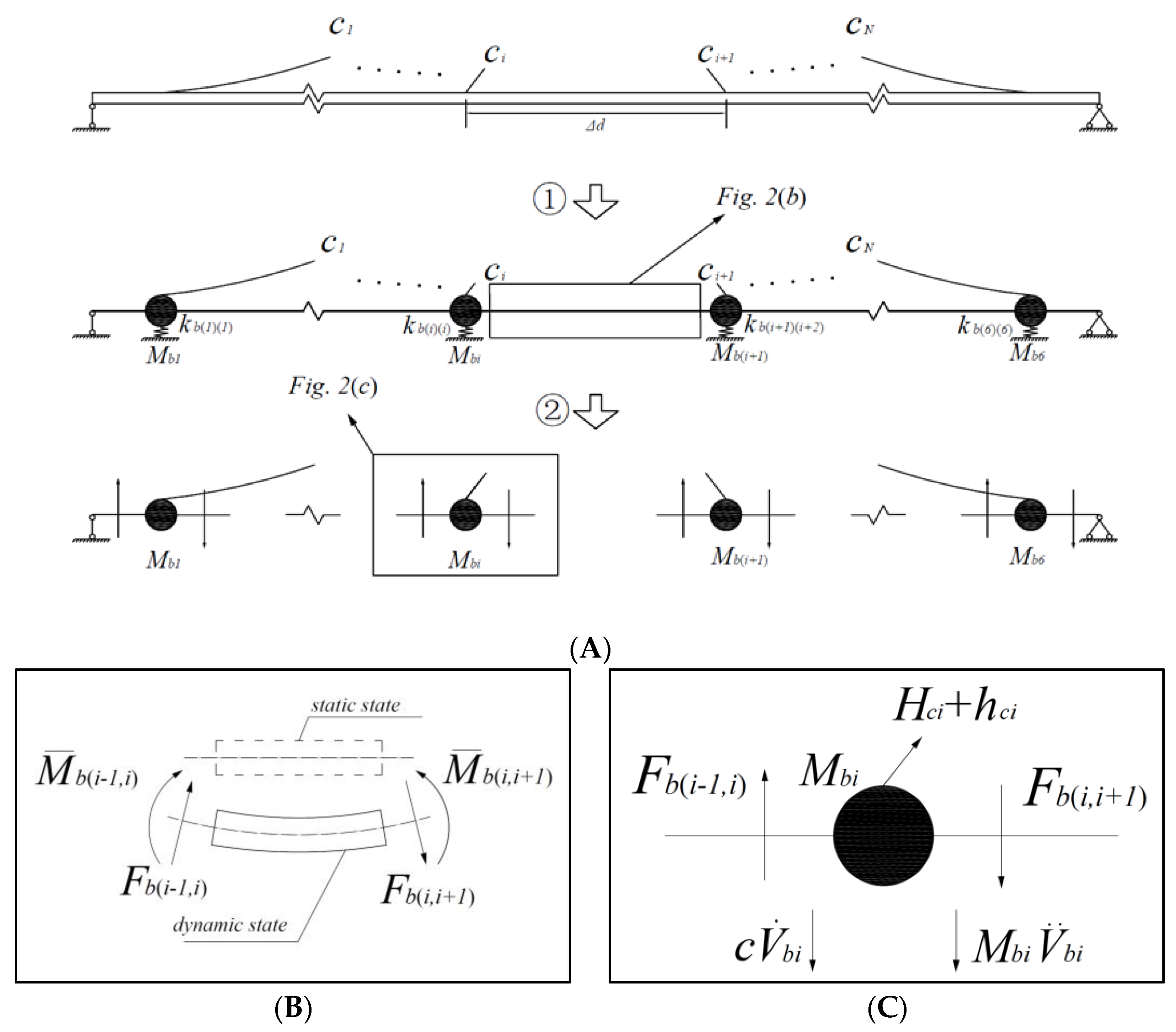
2.2. The Reduced Model of the Beam Considering the CEB

As shown in Figure 1A, the bridge beam is divided into rigid portions connected by springs and hinges. However, for a Euler–Bernoulli beam with distributed mass and distributed load, the plastic material properties hypothesis focused on a certain point does not represent the CEB as a whole structure, which also carries out onerous works on numerical simulation by establishing thousands of finite element model. To address this problem, the shear difference between the left and the right side of the beam section at each cable anchor position is applied to simulate the CEB [28,29,30]. The refined processes of the reduction are shown in Figure 2A: ① according to the anchoring position of each cable, the single beam is reduced to N discrete beam portions connected by spring hinges. It is assumed that the interval displacement d of adjacent cables stays the same, resulting in that the equivalent mass and length $\mathsf{\Delta }d$ between independent beam sections are also the same. ② The single beam can be reduced to an integrated system comprised of a number of discrete beam portions. In Figure 2B,C, to distinguish it from the mass symbol, where ${\overline{M}}_{b\left(i-1\right)}$, ${\overline{M}}_{bi}$ represent the bending moments on the left and right sides of the section between adjacent beam portions, respectively, and $F_{b\left(i-1,i\right)}$, $F_{b\left(i,i+1\right)}$ represent the shear force on the left and right sides of the beam portion at the cable’s anchored position, respectively.

After considering the equilibrium conditions, the vibration equation of the Bi# beam portion can be obtained by the D’Alembert Principle:

$$M_{bi}·{\ddot{V}}_{bi}\left(t\right)-h_{ci}·sin{\theta }_i+\mathsf{\Delta }{F}_i+c_{bi}·{\dot{V}}_{bi}\left(t\right)=0$$

(16)

where the shear difference $\mathsf{\Delta }{F}_{\left(i\right)}$ represents the influence between different beam portions due to the bending stiffness of a continuous single beam. To reduce the amount of the calculation, the finite difference is also applied to correct the vibration equation of each beam portion. The curvature ${\rho }_{bi}$ and the bending moment ${\overline{M}}_{bi}$ of the Bi# beam portion can be approximated obtained by the second-order central difference:

$${\overline{M}}_{bi}=-E_{bi}{I}_{bi}·{(\frac{1}{\rho })}_{bi}\approx \frac{-E_{bi}{I}_{bi}}{d^2}\left[V_{b\left(i-1\right)}\left(t\right)-2V_{bi}\left(t\right)+V_{b\left(i+1\right)}\left(t\right)\right]$$

(17)

The shear at both sides of the micro-segment satisfies the following equations:

$$\mathsf{\Delta }{F}_i=-F_{b\left(i-1,i\right)}+F_{b\left(i,i+1\right)}$$

(18)

$$F_{b\left(i-1,i\right)}=\frac{{\overline{M}}_{bi}-{\overline{M}}_{bi-1}}{d}$$

(19)

$$F_{b\left(i,i+1\right)}=\frac{{\overline{M}}_{bi+1}-{\overline{M}}_{bi}}{d}$$

(20)

Thus, the influence between different beam portions due to the bending stiffness of a continuous single beam satisfies the equation:

$$\mathsf{\Delta }{F}_i=\frac{EI}{d^3}\left[-V_{b\left(i-2\right)}\left(t\right)+4V_{b\left(i-1\right)}\left(t\right)-6V_{bi}\left(t\right)+4V_{b\left(i+1\right)}\left(t\right)-V_{b\left(i+2\right)}\left(t\right)\right]$$

(21)

It is noticeable that one end of the B1# beam portion and B6# beam portion is close to the simply supported end where the bending moment and displacement are equal to zero. Inserting $\mathsf{\Delta }{F}_i$ into Equation (16), by some simplifications, the vibration equation of the Bi# beam portion can be obtained as follows:

$$\begin{array}{cc}\hfill M_{bi}·{\ddot{V}}_{bi}\left(t\right)+& \frac{E_{ci}^{*}{A}_{ci}}{L_{ci}}si{n}^2{\theta }_i·V_{bi}\left(t\right)+\frac{E_{ci}^{*}{A}_{ci}}{2L_{ci}}sin2{\theta }_i·V_t\left(t\right)-\frac{16D_{ci}{E}_{ci}{A}_{ci}}{\pi L_i{}^2}sin{\theta }_i\hfill \\ & ·V_{ci}\left(t\right)-\frac{{\pi }^2{E}_{ci}{A}_{ci}}{2L_{ci}{}^2}·sin{\theta }_i·V_{ci}{}^2\left(t\right)-\frac{E_{ci}{A}_{ci}}{L_{ci}{}^2}si{n}^3{\theta }_i·V_t{}^2\left(t\right)\hfill \\ & -\frac{E_{ci}{A}_{ci}}{L_{ci}{}^2}sin{\theta }_{i}co{s}^2{\theta }_i·V_{bi}{}^2\left(t\right)+\frac{E_{ci}{A}_{ci}}{2L_{ci}{}^2}sin{\theta }_{i}sin2{\theta }_i\hfill \\ & ·V_{bi}\left(t\right)V_t\left(t\right)+\frac{E_{bi}{I}_{bi}}{d^2}[-V_{b(i-2)}\left(t\right)+4V_{b\left(i-1\right)}\left(t\right)-6V_{bi}\left(t\right)\hfill \\ & +4V_{b\left(i+1\right)}\left(t\right)-V_{b\left(i+2\right)}\left(t\right)] +c_{bi}·{\dot{V}}_{bi}\left(t\right)=0\hfill \end{array}$$

(22)

3. The Mathematical Model of the MCS

3.1. The Equations of the MCS

To avoid repetition, $V_t\left(t\right)$, $V_{ci}\left(t\right)$ and $V_{bi}\left(t\right)$ are all reduced to the symbols $V_t$, $V_{ci}$ and $V_{bi}$. Equations (1) and (15) are reduced to non-dimensional form equations by imposing the Galerkin Method. Summarizing Equation (22), the dynamic equations of the whole system can be obtained, as shown in Equation (23):

$$\begin{array}{cc}\hfill {\ddot{V}}_t+{\alpha }_1·V_t+{\alpha }_2& ·\dot{V}+{\alpha }_3·V_t{}^2+{\alpha }_4·V_{bi}+{\alpha }_5·V_{bi}{}^2+{\alpha }_6·V_{ci}+{\alpha }_7·V_{ci}{}^2+{\alpha }_8\hfill \\ & ·V_{bi}{V}_t+{\alpha }_8=0\hfill \end{array}$$

(23)

$$\begin{array}{cc}\hfill {\ddot{\mathit{V}}}_{\mathit{c}\mathit{i}}+{\mathsf{\beta }}_{\mathbf{1}}^{\mathit{i}}·{\mathit{V}}_{\mathit{c}\mathit{i}}+& {\mathsf{\beta }}_{\mathbf{2}}^{\mathit{i}}·{\ddot{\mathit{V}}}_{\mathit{b}\mathit{i}}+{\mathsf{\beta }}_{\mathbf{3}}^{\mathit{i}}·{\ddot{V}}_t+{\mathsf{\beta }}_{\mathbf{4}}^{\mathit{i}}·{\dot{\mathit{V}}}_{\mathit{c}\mathit{i}}+{\mathsf{\beta }}_{\mathbf{5}}^{\mathsf{i}}·{\dot{\mathit{V}}}_{\mathit{b}\mathit{i}}+{\mathsf{\beta }}_{\mathbf{6}}^{\mathit{i}}·{\dot{V}}_t+{\mathsf{\beta }}_{\mathbf{7}}^{\mathit{i}}·{\mathit{V}}_{\mathit{c}\mathit{i}}{}^{\mathbf{2}}\hfill \\ & +{\mathsf{\beta }}_{\mathbf{8}}^{\mathit{i}}·{\mathit{V}}_{\mathit{c}\mathit{i}}{}^3+{\mathsf{\beta }}_{\mathbf{9}}^{\mathit{i}}·{\mathit{V}}_{\mathit{b}\mathit{i}}+{\mathsf{\beta }}_{10}^{\mathit{i}}·V_t+{\mathsf{\beta }}_{11}^{\mathit{i}}·V_t{}^2+{\mathsf{\beta }}_{\mathbf{12}}^{\mathit{i}}·{\mathit{V}}_{\mathit{b}\mathit{i}}{}^{\mathbf{2}}+{\mathsf{\beta }}_{\mathbf{13}}^{\mathit{i}}\hfill \\ & ·{\mathit{V}}_{\mathit{b}\mathit{i}}·V_t+\left[{\mathsf{\beta }}_{\mathbf{14}}^{\mathit{i}}\right]·\left\{{\mathit{V}}_{\mathit{b}}{\mathit{V}}_{\mathit{c}\mathit{i}}\right\}+\left[{\mathsf{\beta }}_{\mathbf{15}}^{\mathit{i}}\right]·\left\{{\mathit{V}}_{\mathit{c}\mathit{i}}\right\}·V_t+{\mathsf{\beta }}_{\mathbf{16}}^{\mathit{i}}·{\mathit{V}}_{\mathit{c}\mathit{i}}·V_t{}^2\hfill \\ & +{\mathsf{\beta }}_{\mathbf{17}}^{\mathit{i}}·{\mathit{V}}_{\mathit{b}\mathit{i}}{}^{\mathbf{2}}{\mathit{V}}_{\mathit{c}\mathit{i}}+{\mathsf{\beta }}_{\mathbf{18}}^{\mathit{i}}·{\mathit{V}}_{\mathit{b}\mathit{i}}{\mathit{V}}_{\mathit{c}\mathit{i}}·V_t=0\hfill \end{array}$$

(24)

$$\begin{array}{cc}\hfill {\ddot{\mathit{V}}}_{\mathit{b}\mathit{i}}+{\mathsf{\gamma }}_{\mathbf{1}}^{\mathit{i}}·{\mathit{V}}_{\mathit{b}\mathit{i}}+& {\mathsf{\gamma }}_2^i·{\dot{\mathit{V}}}_{\mathit{b}\mathit{i}}+{\mathsf{\gamma }}_{\mathbf{3}}^{\mathit{i}}·{\mathit{V}}_{\mathit{b}\mathit{i}}{}^2+{\mathsf{\gamma }}_{\mathbf{4}}^{\mathit{i}}·V_t+{\mathsf{\gamma }}_{\mathbf{5}}^{\mathit{i}}·V_t{}^2+{\mathsf{\gamma }}_{\mathbf{6}}^{\mathit{i}}·{\mathit{V}}_{\mathit{c}\mathit{i}}+{\mathsf{\gamma }}_{\mathbf{7}}^{\mathit{i}}·{\mathit{V}}_{\mathit{c}\mathit{i}}{}^{\mathbf{2}}\hfill \\ & +{\mathsf{\gamma }}_{\mathbf{8}}^{\mathit{i}}·{\mathit{V}}_{\mathit{b}\mathit{i}}·V_t+\frac{EI}{d^2}·\mathit{D}·\frac{{\mathit{V}}_{\mathit{b}\mathit{i}}}{{\mathit{M}}_{\mathit{b}\mathit{i}}}=0\hfill \end{array}$$

(25)

where ${\ddot{\mathit{V}}}_{\mathit{c}\mathit{i}}$, ${\ddot{\mathit{V}}}_{\mathit{b}\mathit{i}}$, ${\dot{\mathit{V}}}_{\mathit{c}\mathit{i}}$, ${\dot{\mathit{V}}}_{\mathit{b}\mathit{i}}$, ${\mathit{V}}_{\mathit{c}\mathit{i}}$, ${\mathit{V}}_{\mathit{b}\mathit{i}}$, ${\mathit{V}}_{\mathit{c}\mathit{i}}{}^{\mathbf{2}}$, ${\mathit{V}}_{\mathit{c}\mathit{i}}{}^3$, ${\mathit{V}}_{\mathit{b}\mathit{i}}{}^{\mathbf{2}}$, ${\mathit{V}}_{\mathit{b}}{\mathit{V}}_{\mathit{c}\mathit{i}}$, ${\mathit{V}}_{\mathit{b}\mathit{i}}{}^{\mathbf{2}}{\mathit{V}}_{\mathit{c}\mathit{i}}$ and ${\mathit{V}}_{\mathit{b}\mathit{i}}{}^{\mathbf{2}}$ are 6-element vector column vectors of the same form. To avoid repetition, only the vector of ${\ddot{\mathit{V}}}_{\mathit{c}\mathit{i}}$ is shown as in Equation (26):

$${\ddot{\mathit{V}}}_{\mathit{c}\mathit{i}}={\left\{{\ddot{V}}_{c1},{\ddot{V}}_{c2},{\ddot{V}}_{c3},{\ddot{V}}_{c4},{\ddot{V}}_{c5},{\ddot{V}}_{c6} \right\}}^T$$

(26)

In Equations (24) and (25), ${\mathit{\beta }}_{\mathbf{1}}^{\mathit{i}}$, ${\mathsf{\beta }}_{\mathbf{2}}^{\mathit{i}}$, ${\mathsf{\beta }}_{\mathbf{3}}^{\mathit{i}}$, ${\mathsf{\beta }}_{\mathbf{4}}^{\mathit{i}}$, ${\mathsf{\beta }}_{\mathbf{5}}^{\mathit{i}}$, ${\mathsf{\beta }}_{\mathbf{6}}^{\mathit{i}}$, ${\mathsf{\beta }}_{\mathbf{7}}^{\mathit{i}}$, ${\mathsf{\beta }}_{\mathbf{8}}^{\mathit{i}}$, ${\mathsf{\beta }}_{\mathbf{9}}^{\mathit{i}}$, ${\mathsf{\beta }}_{\mathbf{10}}^{\mathit{i}}$, ${\mathit{\beta }}_{\mathbf{11}}^{\mathit{i}}$, ${\mathsf{\beta }}_{\mathbf{12}}^{\mathit{i}}$, ${\mathsf{\beta }}_{\mathbf{13}}^{\mathit{i}}$, ${\mathsf{\beta }}_{\mathbf{14}}^{\mathit{i}}$, ${\mathsf{\beta }}_{\mathbf{15}}^{\mathit{i}}$, ${\mathsf{\beta }}_{\mathbf{16}}^{\mathit{i}}$, ${\mathsf{\beta }}_{\mathbf{17}}^{\mathit{i}}$, ${\mathsf{\beta }}_{\mathbf{18}}^{\mathit{i}}$, ${\mathsf{\gamma }}_{\mathbf{1}}^{\mathit{i}}$, ${\mathsf{\gamma }}_{\mathbf{2}}^{\mathit{i}}$, ${\mathsf{\gamma }}_{\mathbf{3}}^{\mathit{i}}$, ${\mathsf{\gamma }}_{\mathbf{4}}^{\mathit{i}}$, ${\mathsf{\gamma }}_{\mathbf{5}}^{\mathit{i}}$, ${\mathsf{\gamma }}_{\mathbf{6}}^{\mathit{i}}$, ${\mathsf{\gamma }}_{\mathbf{7}}^{\mathit{i}}$ and ${\mathsf{\gamma }}_{\mathbf{8}}^{\mathit{i}}$ are sixth-order coefficient diagonal matrices of the same form. To avoid repetition, only the matrix of ${\mathsf{\beta }}_{\mathbf{1}}^{\mathit{i}}$ is shown as Equation (27):

$${\mathsf{\beta }}_{\mathbf{1}}^{\mathit{i}}=\left[\begin{array}{cccccc}{\beta }_1^1& & & & & \\ & {\beta }_1^2& & & & \\ & & {\beta }_1^3& & & \\ & & & {\beta }_1^4& & \\ & & & & {\beta }_1^5& \\ & & & & & {\beta }_1^6\end{array}\right]$$

(27)

In Equation (25), $\mathit{D}$ is the coefficient matrix, as shown in Equation (28):

$$\mathit{D}=\left[\begin{array}{cccccc}0& -4& 1& & & \\ -4& 0& -4& 1& & \\ 1& -4& 0& -4& 1& \\ & 1& -4& 0& -4& 1\\ & & 1& -4& 0& -4\\ & & & 1& -4& 0\end{array}\right]$$

(28)

In Equation (25), $\frac{{\mathit{V}}_{\mathit{b}\mathit{i}}}{{\mathit{M}}_{\mathit{b}\mathit{i}}}$ is a 6-dimensional column vector, as shown in Equation (29):

$$\frac{{\mathit{V}}_{\mathit{b}\mathit{i}}}{{\mathit{M}}_{\mathit{b}\mathit{i}}}={\left\{\frac{V_{b1}}{M_{b1}},\frac{V_{b2}}{M_{b2}},\frac{V_{b3}}{M_{b3}},\frac{V_{b4}}{M_{b4}},\frac{V_{b5}}{M_{b6}},\frac{V_{b6}}{M_{b6}} \right\}}^T$$

(29)

The detailed polynomial coefficients in Equation (23) to Equation (25) are given in Appendix B.

In Equation (23) to Equation (25), it is illustrated that a coupling relationship is generated between the vibration equations of the tower and the Bi# beam portion through the dynamic tension $h_{ci}$ of the cable. The geometric nonlinearity of the system is clear with the existence of second-order polynomials and third-order polynomials.

In addition, ${\alpha }_1$, ${\beta }_1^i$ and ${\gamma }_1^i$ represent the polynomial coefficients of parameter incentives [4,8] in the left side of the vibration equation of the tower, the Ci# cable and the Bi# beam portion, respectively. The dimensions of these three coefficients are equal to the square of the natural vibration frequency, named as the dynamic parameters of the tower, Ci# cable and Bi# beam portion participating in the global vibration in the full-bridge dynamic model in this paper, respectively. Once the stiffness restoring force of the beam portion and the sag of the cable is ignorable ($\mu =0$ and neglecting the $sin{\theta }_i$), the coefficient of ${\gamma }_1^i$ is degenerated to the square of the natural frequency equation of the M2 vibrator (${\gamma }_1^i$ = ${\omega }_2{}^2$) in [4]; once the CEB of the bending stiffness of the single beam is ignorable, the coefficient of ${\gamma }_1^i$ is degenerated to the square of the natural frequency equation of the beam (${\gamma }_1^i$ = ${\omega }_{\mathrm{b}}{}^2$) in [9,31]. Compared with the previous references, the reduced model proposed in this paper considers more parameters, and thus the model is closer to the actual bridges.

3.2. The Case Verification

The case of a double-cable structure in [25] and the case of the three-cable structure in [31] are devoted to verifying the effectiveness of the dynamic model and the analytical method in this paper. The key idea of the verification is to reduce the MCS model of this paper into the case model of these two references and compare the calculation results after substituting the parameters of these two references. Without considering the constant coefficient, a logic operation model for numerical simulation based on SIMULINK/MATLAB is established with the Fourth Runge–Kutta method. The initial displacement of each component is selected as 0.01 m, while the fixed-step is selected as 0.01 s. The validity and correctness of the dynamic model proposed in this paper are verified by comparing the vibration displacement curves. The calculation results through the method of this paper (symbolized as PMS in

Table 2. The comparison of the self-vibration frequency calculated by different methods.

Provenance	Shorthand	$\mathbf{Dynamic} \mathbf{Parameter} (\sqrt{{\mathit{\beta }}_1^1}, \mathbf{rad}/\mathbf{s})$
		RMS	PMS
The case of double-cable tructure in [25]	S1C1	1.8928	1.8928
	S1C2	1.8925	1.8925
The case of three-cable structure in [31]	S2C1	3.0753	3.0731
	S2C2	3.0659	3.0747
	S2C3	3.0803	3.0748

) and the references (symbolized as RMS in Table 2) are selected in Table 2.

In Table 2, without considering the influence of gravity on the cable’s vibration, the calculation results in this paper are basically consistent with the results of related references. For further comparison, two conditions (S1 and S2) are considered:

(i)

Ignoring the vibration displacement of the tower ($V_t=0$ in Equation (24)), selecting the parameters in Reference [25] to satisfy the equation $\sqrt{{\beta }_1}\approx 2\sqrt{{\gamma }_1^1}\ne 2\sqrt{{\gamma }_1^2}$ and comparing with the Figure 3 of Reference [25];

(ii)

Selected parameters in [31] to satisfy the equation $\sqrt{{\alpha }_1}\approx \sqrt{{\beta }_1^1}\approx \sqrt{{\beta }_1^2}\approx \sqrt{{\beta }_1^3}$ and compare with the Figures 6–8 of [31]. The vibration displacement comparison of C1# cable is selected under different conditions, as shown in Figure 3.

In Figure 3, although the phases and the maximum amplitudes of these two vibration displacement curves exhibit the difference to some extent, the curve change rules and coupling characteristics of the two calculation cases are quite similar. It is evident from the results that the reduced model proposed in this paper can accurately the simulate dynamic behavior of the MCS. Otherwise, during the verification process, it was found that the methods proposed in the [25,31] did not consider the interaction caused by the CEB when the adjacent cables resonated. More specifically, the numerical analysis of the full-bridge resonance in these two references is adopted under the theoretically given conditions. This is also the target problem addressed in this article.

4. The Numerical Analysis

4.1. Parameters of the Case

As shown in Figure 3, the symmetrical cable and its anchored beam portion are selected with the same parameters. The parameters of the cables are consulted with [9,32], which are also referred from the actual bridges. The basic parameters of each component are presented in

Table 3. Basic parameters of bridge tower and beam sections.

Parameters (Unit)	Tower	Parameters (Unit)	Bi# Beam Portion
$m_t$ (kg/m)	850,000	$M_t$ (kg/m)	250,000
		$E_{bi}$ (MPa)	500
$E_t$ (MPa)	450	$I_{bi}$ (m4)	2.85
		$d_i$ (m)	50
$I_t$ (m4)	3.0	$\sqrt{{\gamma }_1^i}$	B1#	0.2483
			B2#	0.2582
$L_t$ (m)	80		B3#	0.1947
			B4#	0.1947
$\sqrt{{\alpha }_1}$	0.2368		B5#	0.2582
			B6#	0.2483

and

Table 4. Basic parameters of stay cables.

Parameters (Unit)	C1#	C2#	C3#	C4#	C5#	C6#
${\theta }_i$ (rad)	0.57	0.82	1.27	1.27	0.82	0.57
$L_i$ (m)	148.41	109.67	83.82	83.82	109.67	148.41
$A_{ci}$ (cm2)	99.43	70.18	53.49	53.49	70.18	99.43
$H_{ci}$ (MN)	3.88	3.65	3.49	3.49	3.65	3.88
$m_{ci}$ (kg/m)	81.04	57.20	43.59	43.59	57.20	81.04
$D_{ci}$ (m)	0.51	0.16	0.03	0.3	0.16	0.51
$E_{ci}^{*}$ (GPa)	202	208	209	209	208	202
The Irvine Parameter λ [32]	0.3848	0.0538	0.0017	0.0017	0.0538	0.3848
$\sqrt{{\beta }_1^i}$	0.7478	1.1542	1.6891	1.6891	1.1542	0.7478

.

From Table 3, it is noticeable that the values of $E_t{I}_t$ and $E_{bi}{I}_{bi}$ are set relatively lower than the parameters of actual bridges to meet the requirements of the working conditions.

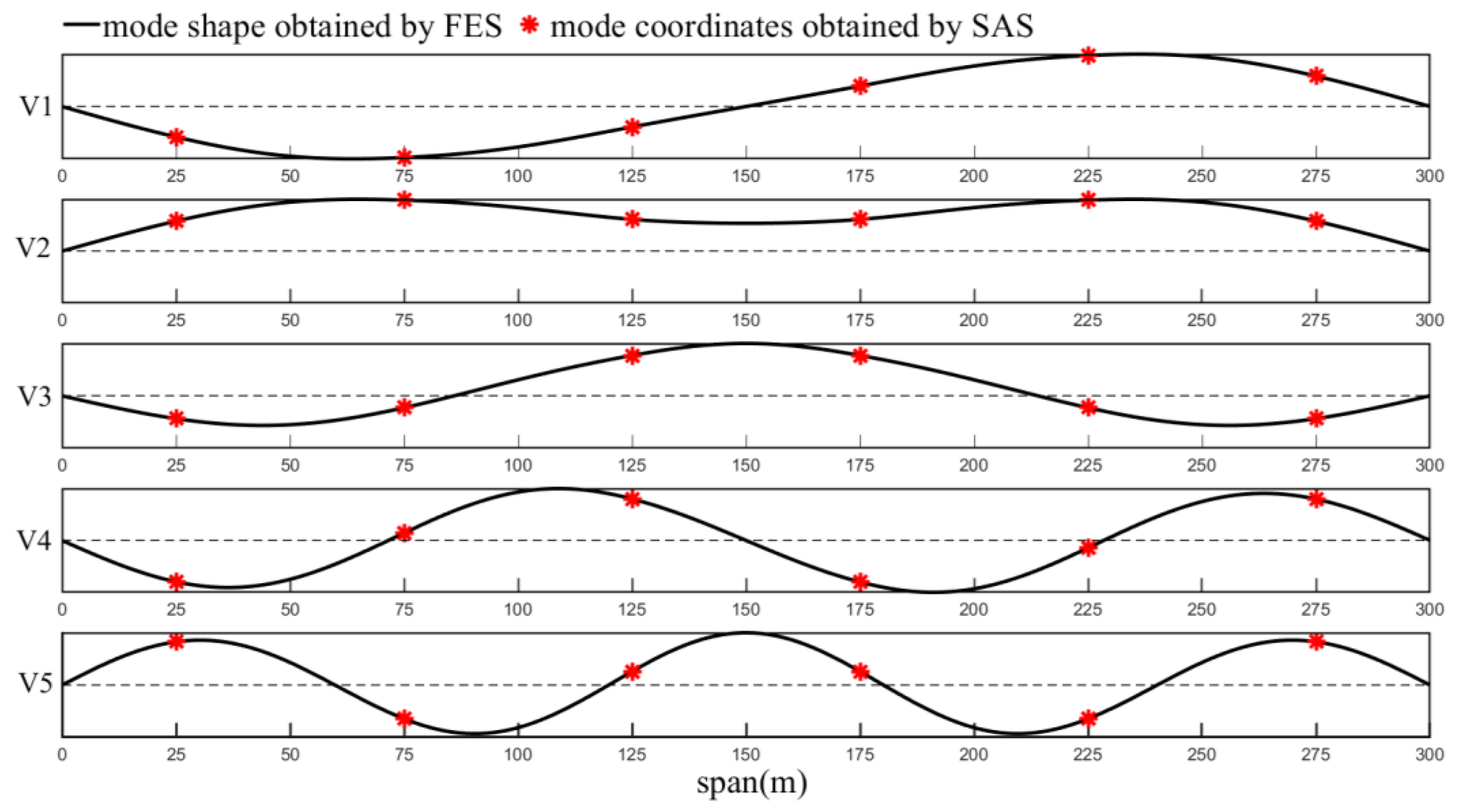
4.2. The In-Plane Vertical Natural Vibration Mode

To accurately analyze the natural vibration mode of the in-plane vertical mode, the MCS is also analyzed through the finite element method (FEM) by commercial software (MIDAS CIVIL). The tower and the beam are all performed by the beam element while the cable is performed by the truss element. The in-plane vertical natural vibration frequencies are selected in

Table 5. The in-plane vertical model properties of the MCS.

Mode No.	Abbreviation	f (Hz)		Error (%)
		FEM	PMS
1	V1	0.01308	0.01309	0.8
2	V2	0.01339	0.01340	0.7
3	V3	0.01780	0.01781	0.6
4	V4	0.02457	0.02459	0.8
5	V5	0.03452	0.03453	0.3

, while the vertical modal shapes of the first five orders are selected as shown in Figure 4, respectively.

In Table 5, the calculation errors with these two methods varied within a small margin. There is little difference between the first two modes of the dynamic system. Additionally, in Figure 4, the vertical mode shapes obtained by PMS fit those obtained by FEM well. It is illustrated that the fundamental vibration shapes and frequencies of the components occupying lower-order modes are not much different. Additionally, it is evident from the comparison of the results that the dynamic model and the numerical analysis in this paper can accurately simulate the CEB.

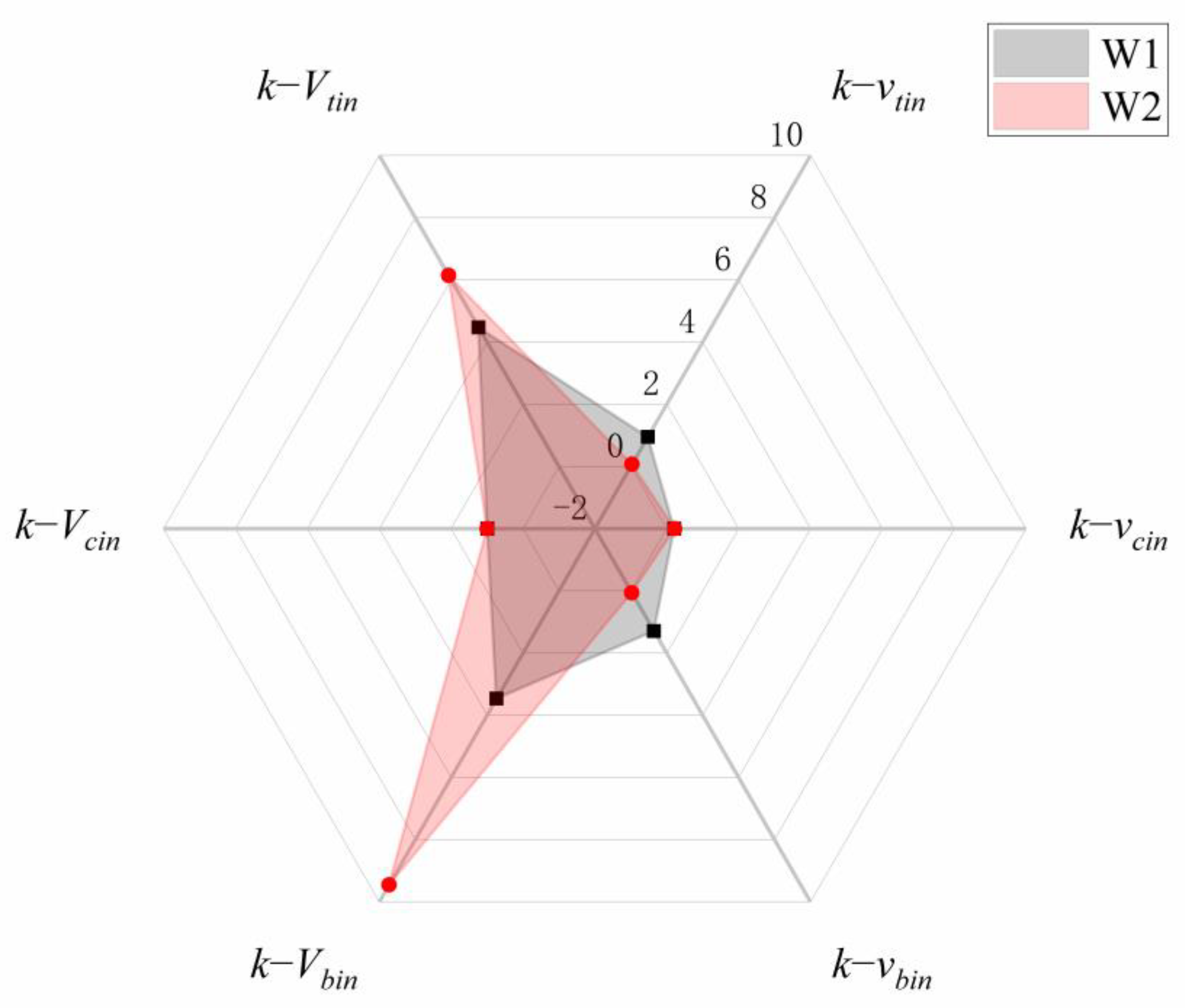
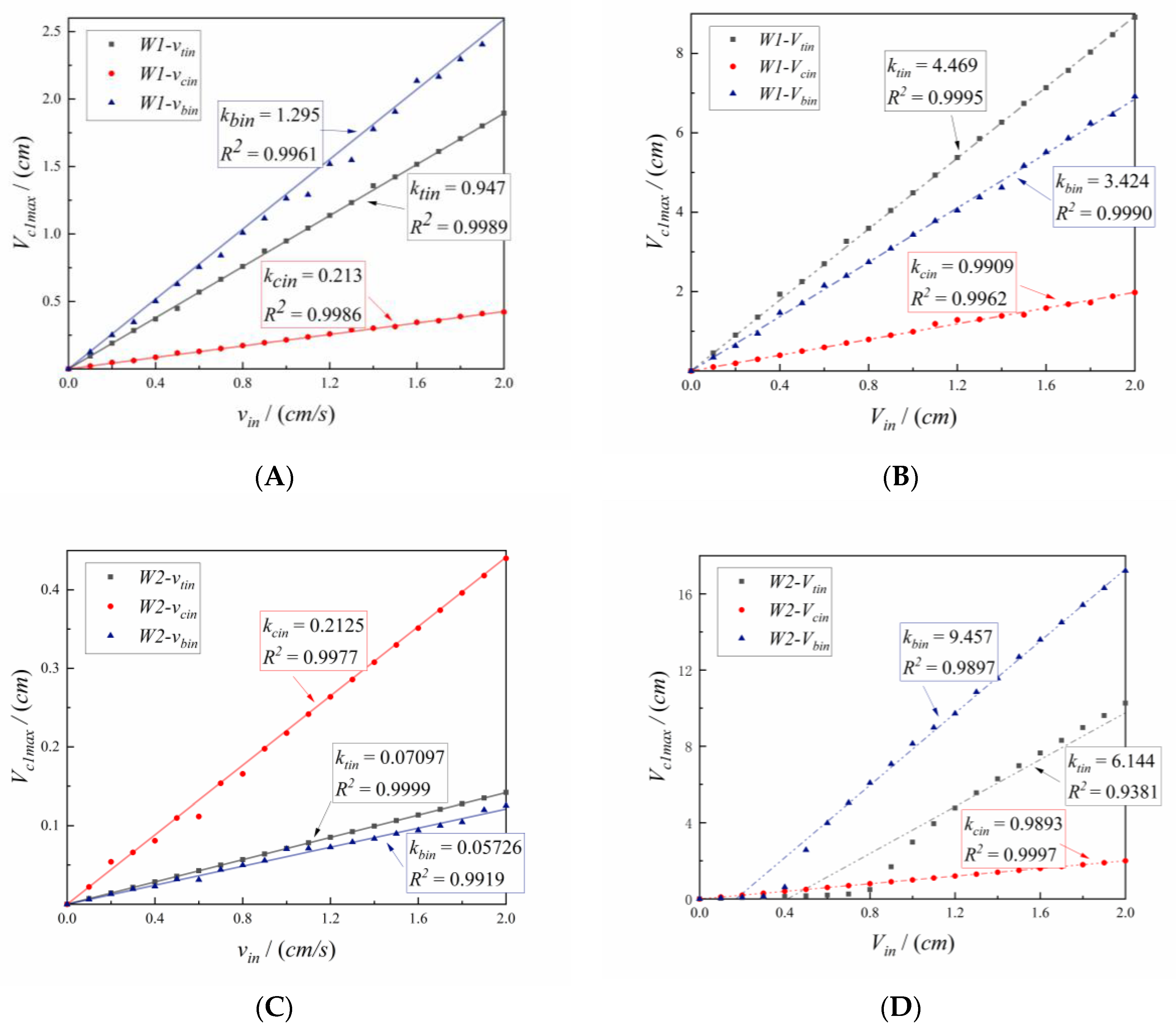
4.3. The Numerical Analysis of the Dynamic Parameter

In this part, sub-system #1 is selected as the research object to apply the numerical analysis. The Fast Fourier Transform method is applied to obtain the spectrogram of different components in sub-system #1. To further verify the effectiveness of the model proposed in this paper on the dynamic analysis, changing the dynamic parameter of each component with variable properties, the dynamic parameter ratio of the tower, cable and beam is deeply discussed through three working conditions which have been widely verified to be the parametric resonance conditions [8,9,11,17,28,31]:

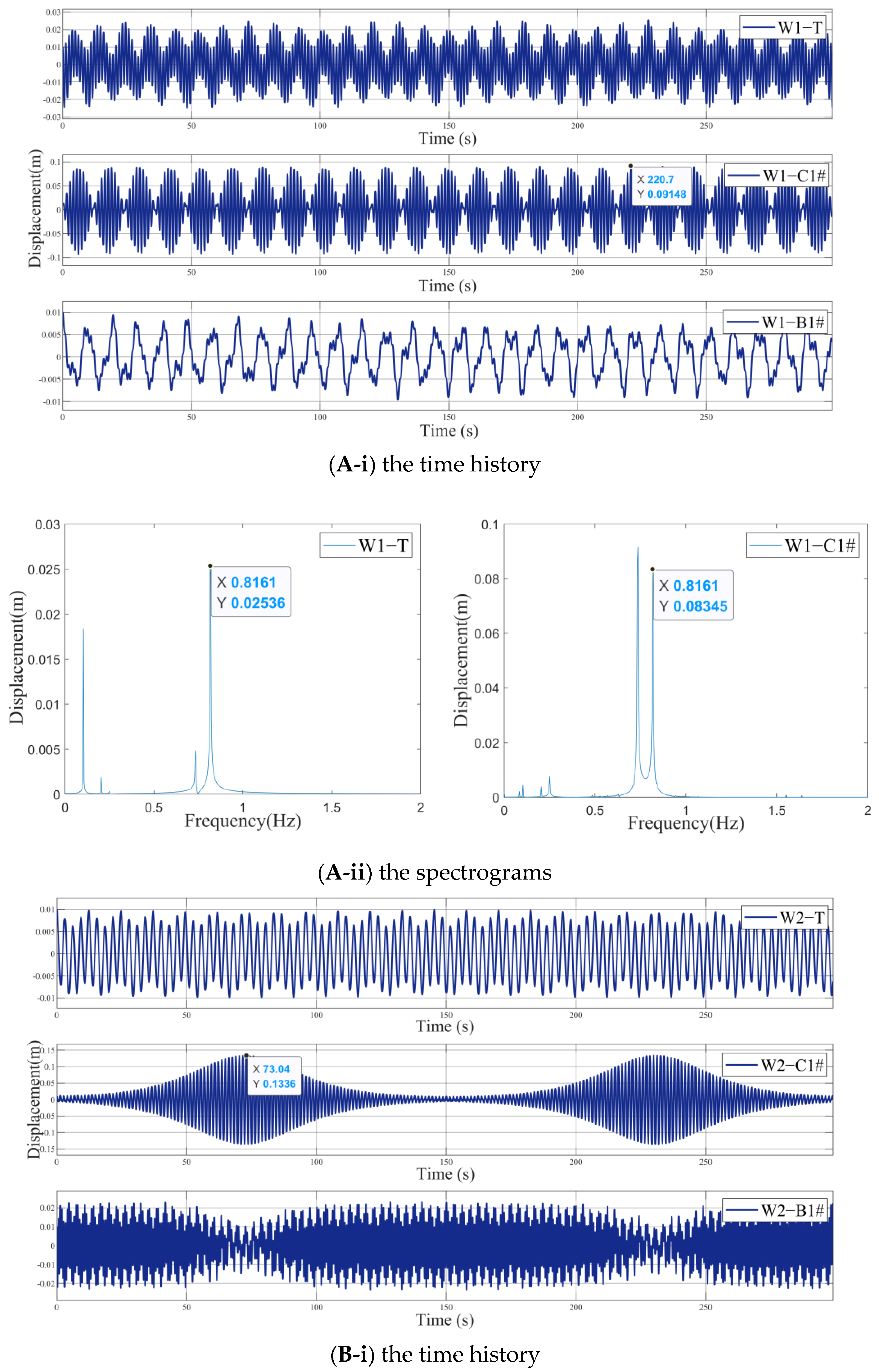
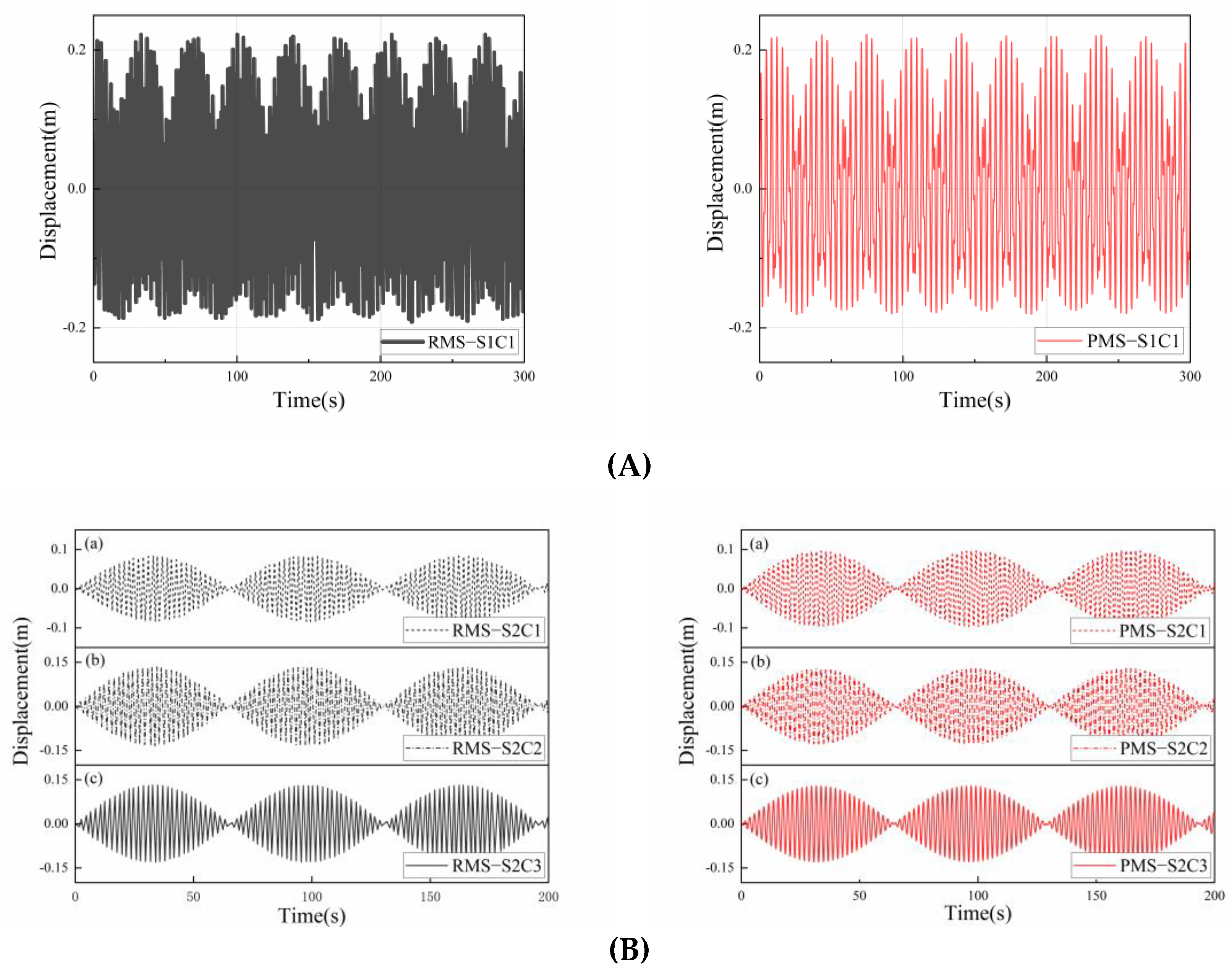
• The first working condition (W1): change $m_t=\mathrm{85,000} \mathrm{kg}/\mathrm{m}$ to satisfy the equation $\sqrt{{\alpha }_1}$:$\sqrt{{\beta }_1^i}\approx 1:1$, and the displacement and the spectrogram of each component is obtained, as shown in Figure 5A;
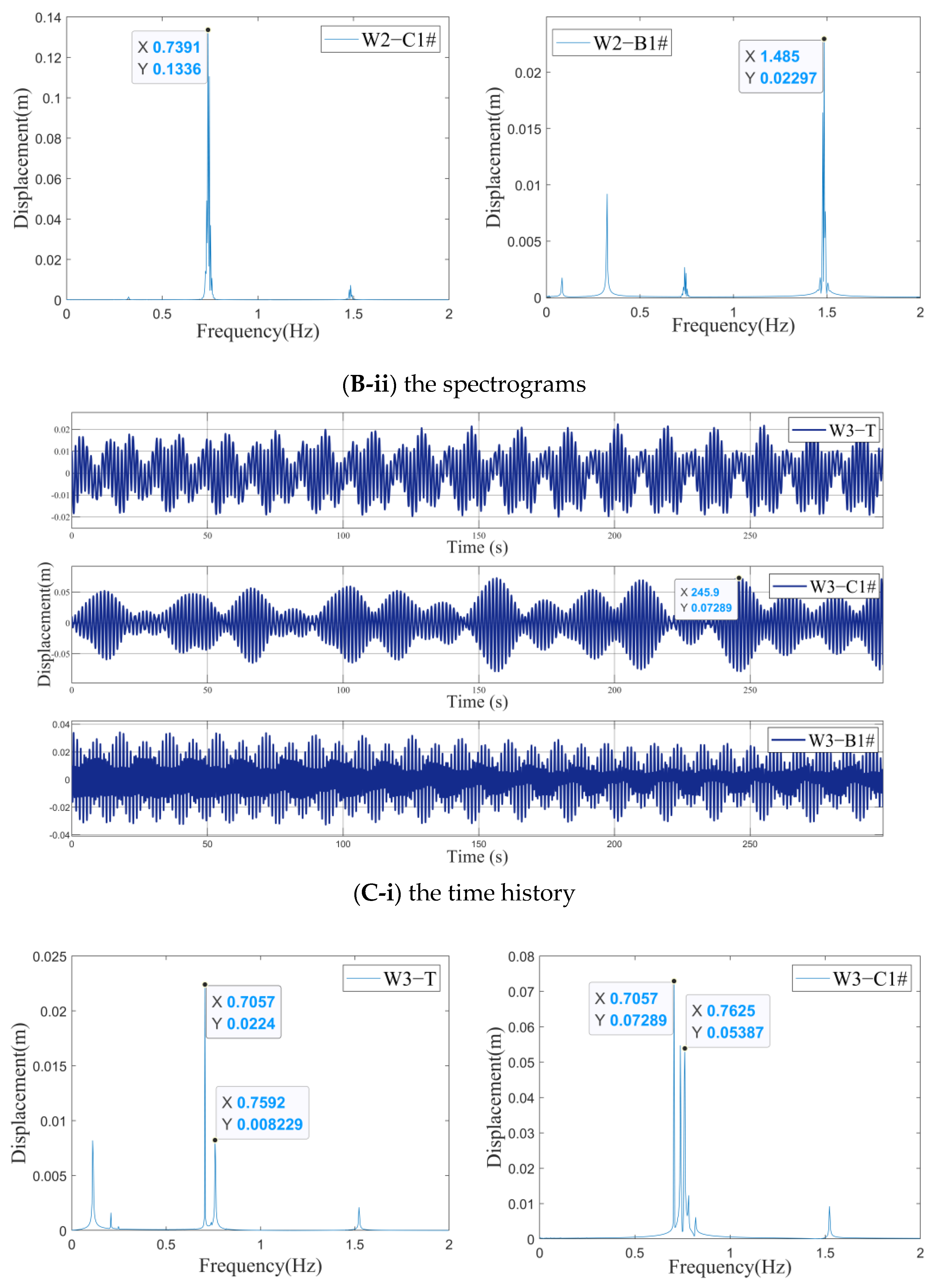
• The second working condition (W2): change $M_{bi}=\mathrm{70,000} \mathrm{kg}$ to satisfy the equation $\sqrt{{\beta }_1^i}$:$\sqrt{{\gamma }_1^i}\approx 1:2$, and the displacement and the spectrogram of each component is obtained, as shown in Figure 5B;
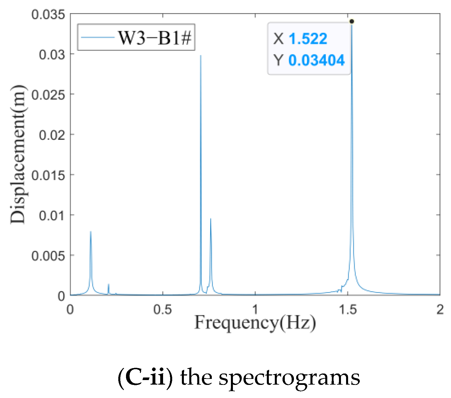
• The third working condition (W3): change $m_t$ and $M_{bi}$ at the same time to satisfy the equation $\sqrt{{\alpha }_1}:\sqrt{{\beta }_1^i}$:$\sqrt{{\gamma }_1^i}\approx 1:1:2$, and the displacement and the spectrogram of each component are obtained, as shown in Figure 5C.

By applying the Fourth Runge–Kutta method on the undamped model, the initial displacement of each component is selected as 0.01 m, while the fixed-step is selected as 0.02 s. The analytical results of the above three conditions are shown in Figure 5.

In Figure 5, it is illustrated that the resonance of the Tower–Cable or Cable–Beam would respectively be observed when the equation of $\sqrt{{\alpha }_1}$:$\sqrt{{\beta }_1^i}$≈1:1 or $\sqrt{{\beta }_1^i}$:$\sqrt{{\gamma }_1^i}$≈1:2 is satisfied. In Figure 5A, when $\sqrt{{\alpha }_1}$:$\sqrt{{\beta }_1^i}$≈1:1 is satisfied, the coupled resonance can be observed from the displacement curves between the tower and the C1# cable. A significant characteristic of the ‘beat’ can be observed on the cable displacement curve. From the spectrogram in Figure 5A, when the vibration frequency of the tower ($f_{\mathrm{t}}=0.8161 \mathrm{Hz}$ or $\mathrm{or} 0.8161 \mathrm{Hz}$) changes to the same value as the C1# cable ($f_{\mathrm{C}1\#}=0.8161 \mathrm{Hz}$), the cable amplitude reaches the peak of the maximum, which is 9.148 times the initial amplitude; in Figure 5B, when $\sqrt{{\beta }_1^i}$:$\sqrt{{\gamma }_1^i}\approx 1:2$ is satisfied, the coupled resonance can be observed from the displacement curves of the C1# cable and the B1# beam portion. In addition, from the spectrogram in Figure 5B, when the vibration frequency of the C1# cable ($f_{\mathrm{C}1\#}=0.7391 \mathrm{Hz}$) changes to nearly half the value of the B1# beam portion ($f_{\mathrm{B}1\#}=1.485 \mathrm{Hz}$), the cable amplitude reaches the peak of the maximum, which is 13.36 times the initial amplitude. Particularly in Figure 5C, the condition is regarded as the special working condition of the parametric resonance. Under this condition, the total energy conversion trans between the tower, the cable and the beam. From the spectrogram in Figure 5C, it is clear that the resonance modes in the system are extremely rich. Different resonances influence and interfere with each other while obtaining a lower maximum amplitude, 7.289 times initial amplitude, than the first two conditions. In general, the parameter of ${\alpha }_1$, ${\beta }_1^i$ and ${\gamma }_1^i$ characterize the ability of different components to participate in the global resonance to a certain extent and are evidently important parameters for the dynamic design of cable-stayed bridges.

5. The Influence Discussion on the Internal Resonance under Different Excitations

To accurately analyze the influence of the different excitations from different components on the parametric resonance, the controlled variable method is applied and the conditions of W1 and W2 are selected. The initial velocity (v_in) or initial displacement (V_in) of the tower, the cable and beam in subsystem #1 is changed from 0 m to 0.02 m, respectively. It is noticeable that the subscript indicates the initial state of the parameter. The maximum value (V_c1max) of the different components under these two conditions and the fitting curves are selected, as shown in Figure 6.

From Figure 6, the correlation coefficients of the fitting R²$\in \left[0.9381,0.9999\right]$ show a significant relationship of linear increase. The initial velocity and initial displacement of different components will have different excitation effects on the cable when the parametric resonance is satisfied in this sub-system. Additionally, in Figure 6D, some curves seem to remain at 0 until V_in = 0.8 cm, while it is known that the internal resonance occurs only above a threshold amplitude. To further discuss the influence on the parametric resonance, the correlation coefficients of the influence (k-V_in or k-v_in), also regarded as the slopes of polynomial linear fitting curves, are selected, as shown in Figure 7.

In Figure 7, the axis coordinate range locates at the interval of [–2,10]. The smaller the slope value, the closer to the center point, and the less significant the effect. Based on this, several priority phenomena of resonance excitation in the parametric resonance of MCS can be clearly observed: ① the excitation effect of the initial displacement under the condition of CBR is generally larger than that under the condition of TCR; ② the excitation effect of the initial displacement is generally larger than that of the initial velocity; ③ the excitation sequence of the internal components of the subsystem is: beam > tower > cable; ④ the excitation effect of the initial displacement under the condition of CBR has the most significant influence among the others, whose influence coefficient (k-V_bin) reaches the peak of 9.457.

Additionally, the cable can also be excited by the indirect influence of adjacent cables under the whole condition of MCE. To analyze this effect, the initial displacement of the beam section under the W1 working condition, whose coupling ‘beat’ characteristic is relatively obvious, is applied to the background of the investigation object. The initial displacement of the B1# beam portion, B2# beam portion and B3# beam portion are selected as 0.01 m, while other parameters are selected as 0. The displacement of the C1# cable is shown in Figure 8.

From Figure 8, the cable of the MCS can be excited by the components of other sub-systems through the medium effect of CEB or the tower. The originally static component would be excited to obtain an initial velocity or displacement due to the effect. Moreover, if the sub-system of the exciting cable satisfies the parametric resonance conditions, the effect will be converted into the parametric resonance excitation of the cable, resulting in a severe oscillation. In addition, the closer the beam portion of the resonant subsystem is, the larger the resonance amplitude of the cable. It appears possible that the resonance energy can be transformed to other sub-systems through the CEB. Thus, it is important to focus on the dynamic parameters of the components avoiding the parametric resonance conditions in the design phase.

6. Conclusions

This paper aims to simulate the CEB of the MCS and investigate the excitations of parametric resonance through the defined relationship of the dynamic parameters of different components. To make ODEs more accessible to the numerical simulation, the shear difference and the finite difference method are applied to simulate the CEB of the MCS, whose accuracy and effectiveness have been verified by the case study and the dynamic analysis of mode shapes. A few meaningful conclusions are obtained as follows:

• The CEB, including the effect of bending stiffness of the single beam or indirect influence of adjacent cables, does affect the parametric resonance. The effectiveness of the refined dynamic model considering CEB has been verified by case investigations.
• The concept of dynamic parameters of each component, which affects the conditions of the parametric resonance, is proposed in this paper and deeply discussed with the influence effect on the parametric resonance.
• The excitation effects of different initial conditions are discussed in this paper. The excitation of the beam’s initial displacement under the condition of the CBR, by which the maximum displacement of the cable reaches the peak of 13.36 times the initial value, is relatively large among others. In addition, the different internal resonance behavior of the cable would interfere with each other, resulting in the relatively small maximum vibration displacement of the cable when the CBR and TCR occur at the same time.
• The process of the energy conversion through the medium of the CEB or the tower has been simulated when the parametric resonance occurs. It is evident that the indirect coupling effect of adjacent cables through the beam or the tower cannot be ignored in the parametric resonance of the MCS. Hence, the dynamic analysis of CEB should be paid more attention to the engineering design of the cable-stayed bridge.

The reduced model established in this paper provides an accessible method for investigating the dynamic characteristics of MCS. The next step of the research will focus on the refined simulation of the single beams and the high-order modal nonlinear resonance analysis of the cable.

References

1. Yu, Y.L.; Gao, W.C.; Sun, Y. Study on Refined Model and Influence Factors of Parametric Vibration of Inclined Cables. Eng. Mech. 2010, A02, 178–185. [Google Scholar]
2. Kang, H.J.; Zhu, H.P.; Zhao, Y.Y.; Yi, Z.P. In-Plane Non-Linear Dynamics of the Stay Cables. Nonlinear Dyn. 2013, 73, 1385. [Google Scholar] [CrossRef]
3. Weber, B. Nonlinear Stay Cable–Bridge Deck Interaction. In International Conference on Experimental Vibration Analysis for Civil Engineering Structures; Springer: Cham, Switzerland, 2017. [Google Scholar]
4. Zhu, J.; Ye, G.R.; Xiang, Y.Q.; Chen, W.Q. Non-linear dynamics of cable-stayed beams. J. Zhejiang Univ. (Eng. Sci.) 2010, 44, 2326–2341. [Google Scholar]
5. Fujino, Y.; Kimura, K. Cables and Cable Vibration in Cable-Supported Bridges. In Proceedings of International Seminar on Cable Dynamics, Technical Committee on Cable Structures and Wind; Japan Association for Wind Engineering: Tokyo, Japan, 1997; pp. 1–11. [Google Scholar]
6. Manabe, Y.; Sasaki, N.; Yamaguti, K. Field Vibration Test of the Tatara Bridge. Bridge Found. Eng. 1999, 33, 27–30. [Google Scholar]
7. Caetano, E. Cable Vibrations in Cable-Stayed Bridges; IABSE: Zürich, Switzerland, 2012. [Google Scholar]
8. Kang, Z.; Xu, K.; Luo, Z. A numerical study on nonlinear vibration of an inclined cable coupled with the deck in cable-stayed. J. Vib. Control. 2011, 18, 404–416. [Google Scholar] [CrossRef]
9. Song, M.T.; Cao, D.Q.; Zhu, W.D.; Bi, Q.S. Dynamic response of a cable-stayed bridge subjected to a moving vehicle load. Acta Mech. 2016, 227, 2925–2945. [Google Scholar] [CrossRef]
10. Cong, Y.; Kang, H.; Yan, G.; Guo, T. Modeling, dynamics, and parametric studies of a multi-cable-stayed beam model. Acta Mech. 2020, 231, 4947–4970. [Google Scholar] [CrossRef]
11. Gattulli, V.; Lepidi, M.; Macdonald, J.H.G.; Taylor, C.A. One-to-Two Global-Local Interaction in A Cable-Stayed Beam Observed Through Analytical, Finite Element and Experimental Models. Int. J. Non-Linear Mech. 2005, 40, 571–588. [Google Scholar] [CrossRef]
12. Gattulli, V.; Lepidi, M. Localization and Veering in the Dynamics of Cable-Stayed Bridges. Comput. Struct. 2007, 85, 1661–1678. [Google Scholar] [CrossRef]
13. Wang, F.; Wen, X.X.; Liu, Z.J. Coupled Vibration Analysis of Tower-Cable-Deck of Long-Span Cable-Stayed Bridge. Chin. J. Appl. Mech. 2015, 32, 340–346. [Google Scholar]
14. Sun, C.; Zhao, Y.; Peng, J.; Kang, H.; Zhao, Y. Multiple internal resonances and modal interaction processes of a cable stayed bridge physical model subjected to an invariant single-excitation. Eng. Struct. 2018, 172, 938–955. [Google Scholar] [CrossRef]
15. Sun, C.S.; Zhao, Y.B.; Wang, Z.Q.; Jian, P. Effects of Longitudinal Girder Vibration on Non-Linear Cable Responses in Cable-Stayed Bridges. Eur. J. Environ. Civ. Eng. 2015, 21, 94–107. [Google Scholar] [CrossRef]
16. Zhang, W.J.; Wang, B.; Yang, J.B.; Chai, X.P. Study of Vibration Property of Stay Cables of Jiu-jiang Changjiang River Highway Bridge. World Bridges 2012, 40, 47–51. [Google Scholar]
17. Caetano, E.; Cunha, A.; Gattulli, V.; Lepidi, M. Cable-Deck Dynamic Interactions at the International Guadiana Bridge: On-Site Measurements and Finite Element Modelling. Struct. Control. Health Monit. 2010, 15, 237–264. [Google Scholar] [CrossRef]
18. Ouni, M.; Kahla, N.B.; Preumont, A. Numerical and Experimental Dynamic Analysis and Control of a Cable Stayed Bridge Under Parametric Excitation. Eng. Struct. 2012, 45, 244–256. [Google Scholar] [CrossRef]
19. Ricciardi, G.; Saitta, F. A Continuous Vibration Analysis Model for Cables with Sag and Bending Stiffness. Eng. Struct. 2008, 30, 1459–1472. [Google Scholar] [CrossRef]
20. Lu, Q.; Sun, Z.; Zhang, W. Nonlinear parametric vibration with different orders of small parameters for stayed cables. Eng. Struct. 2020, 224, 111198. [Google Scholar] [CrossRef]
21. Kamel, M.M.; Hamed, Y.S. Nonlinear analysis of an elastic cable under harmonic excitation. Acta Mech. 2010, 214, 315–325. [Google Scholar] [CrossRef]
22. Cong, Y.; Kang, H.; Yan, G. Investigation of dynamic behavior of a cable-stayed cantilever beam under two-frequency excitations. Int. J. Non-Linear Mech. 2021, 129, 103670. [Google Scholar] [CrossRef]
23. Zhao, Y.; Guo, Z.; Huang, C.; Chen, L.; Li, S. Analytical solutions for planar simultaneous resonances of suspended cables involving two external periodic excitations. Acta Mech. 2018, 229, 4393–4411. [Google Scholar] [CrossRef]
24. Yang, S.Z.; Chen, A.R. Parametric Oscillation of Super Long Stay Cables. J. Tongji Univ. (Nat. Sci.) 2005, 10, 27–32. [Google Scholar]
25. Zhao, Y.Y.; Wang, T.; Kang, H.J.; Wang, L.H. Analysis of Nonlinear Parametric Vibration Characteristics of Cable Stayed Bridge w1ith Two Cables Coupled to Deck. J. Hunan Univ. (Nat. Sci.) 2008, 10, 1–5. [Google Scholar]
26. Tagata, G. Harmonically Forced, Finite Amplitude Vibration of a String. J. Sound Vib. 1977, 51, 483–492. [Google Scholar] [CrossRef]
27. Liu, S.L. Cable-Stayed Bridge; People’s Communications Press: Beijing, China, 2002. [Google Scholar]
28. Chen, K.; He, S.; Song, Y.; Wu, L.; Wang, K.; Zhang, H. The Numerical Analysis for Parametric Resonance of Multicable System considering Interaction between Adjacent Beam Portions. Hindawi Shock. Vib. 2021, 2021, 6937794. [Google Scholar] [CrossRef]
29. Turco, E.; Barchiesi, E.; Giorgio, I.; dell’Isola, F. A Lagrangian Hencky-type non-linear model suitable for metamaterials design of shearable and extensible slender deformable bodies alternative to Timoshenko theory. Int. J. Non-Linear Mech. 2020, 123, 103481. [Google Scholar] [CrossRef]
30. Giorgio, I. A discrete formulation of Kirchhoff rods in large-motion dynamics. Math. Mech. Solids 2020, 25, 1081–1100. [Google Scholar] [CrossRef]
31. Tan, C.J.; Zhu, B. Coupling vibration analysis of cable and deck of long-span cable-stayed bridge. J. Southwest Jiaotong Univ. 2007, 06, 726–731. [Google Scholar]
32. Irvine, H.M. Cable Structure; MIT Press: Cambridge, MA, USA, 1981. [Google Scholar]
Figure 1. The schematic diagram of the dynamic model: (A) the reduced model of a dynamic tower–six-cables–beam system; (B) the reduced model of the Ci# cable sub-system; (C) the micro-element section of the cable.
Applsci 12 04095 g001
Figure 2. The reduced model of the Bi# beam portion: (A) The reduced process of the single beam; (B) The schematic diagram of the middle section; (C) The schematic diagram of Bi# beam portion.
Applsci 12 04095 g002
Figure 3. The comparison of simulation results obtained from this paper with other researches: (A) compared with [25]: the vibration displacement comparison of Cable 1 when β 1 2 γ 1 1 2 γ 1 2 ; (B) compared with [31]: the vibration displacement comparison from Cable 1 to Cable 3 when α 1 β 1 1 β 1 2 β 1 3 .
Applsci 12 04095 g003
Figure 4. The in-plane vertical natural vibration mode shapes of the MCS.
Applsci 12 04095 g004
Figure 5. The time and frequency domain diagrams of each degree-of-freedom of subsystem #1 under: (A) W1; (B) W2; (C) W3.
Applsci 12 04095 g005aApplsci 12 04095 g005bApplsci 12 04095 g005c
Figure 6. The influence of initial conditions on the maximum vibration displacement of different components: (A) relationship between vin and Vc1max under W1 condition; (B) relationship between Vin and Vc1max under W1 condition; (C) relationship between vin and Vc1max under W2 condition; (D) relationship between Vin and Vc1max under W2 condition.
Applsci 12 04095 g006
Figure 7. The correlation coefficients of the influence (k-Vin or k-vin) under W1 and W2.
Applsci 12 04095 g007
Figure 8. The displacement of the C1# cable under different initial conditions.
Applsci 12 04095 g008