
Propeller Slipstream Effect on Aerodynamic Characteristics of Micro Air Vehicle at Low Reynolds Number


Abstract
:1. Introduction
2. Computational Framework
2.1. Governing Equations and Solution Details
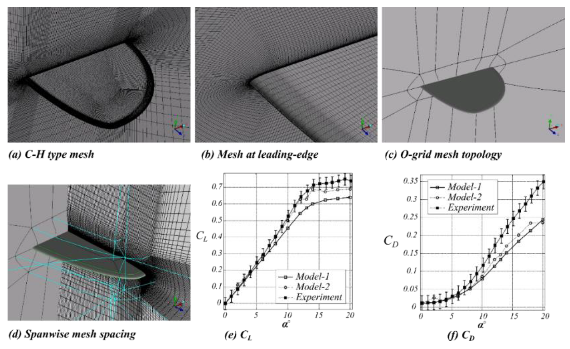
2.2. Specifications of Validation Cases
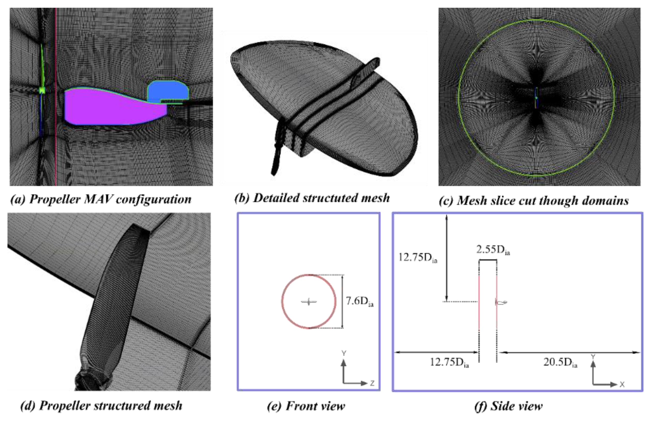
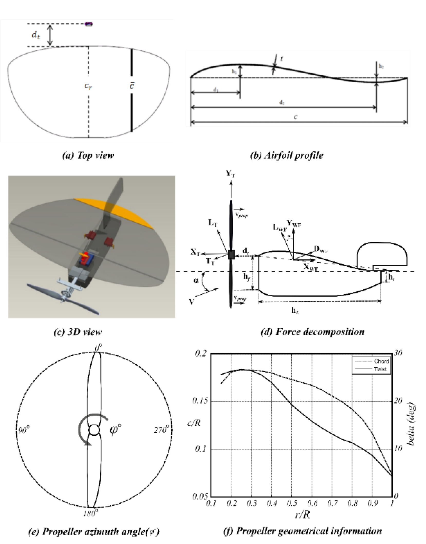
2.3. Present Investigation Case
3. Results and Discussion
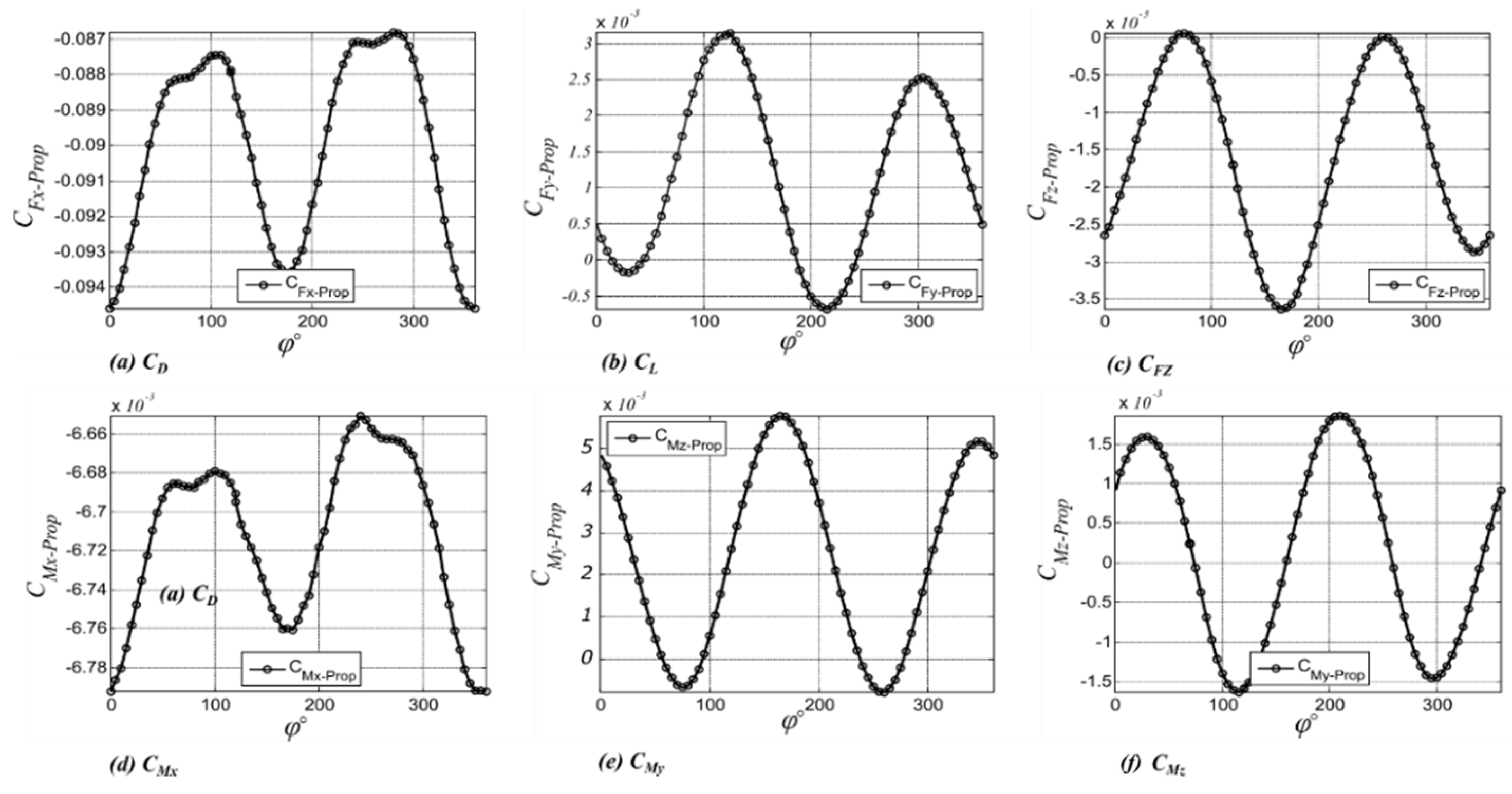
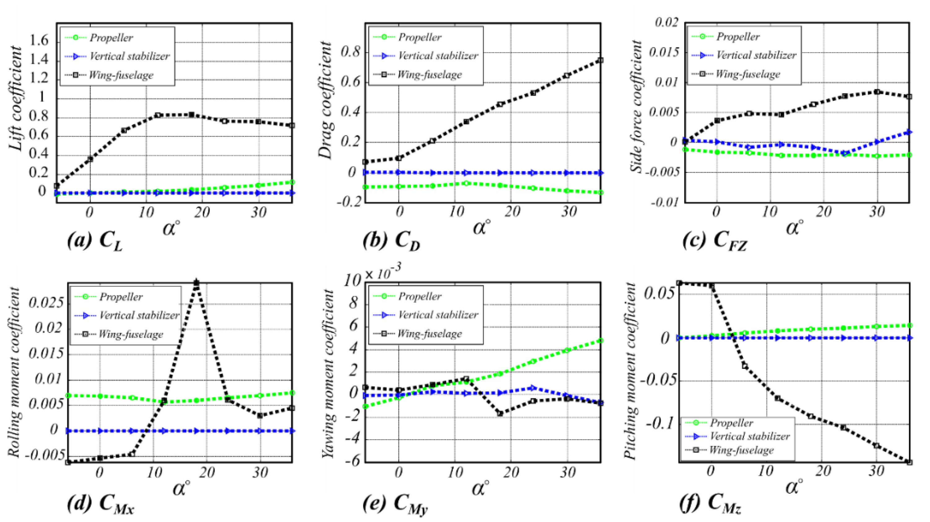
3.1. Propeller Slipstream Effects on Aerodynamic Performance
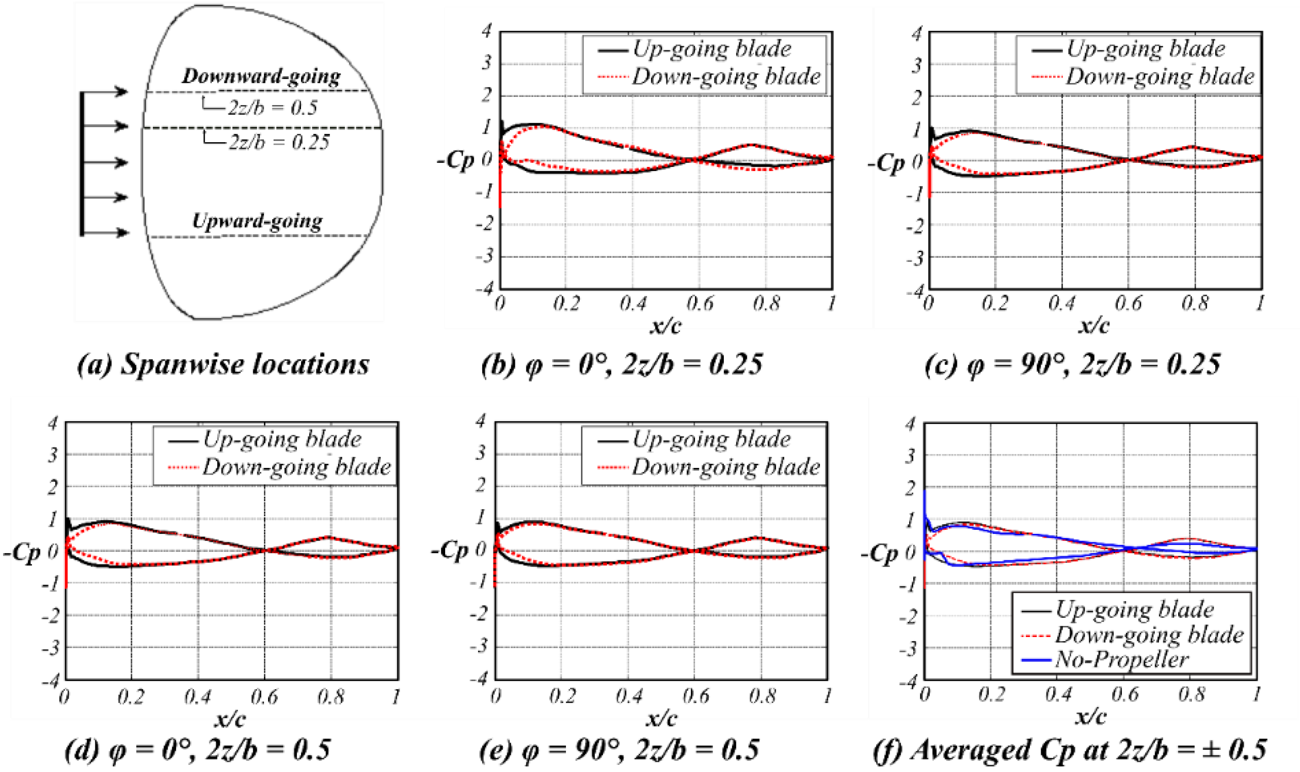
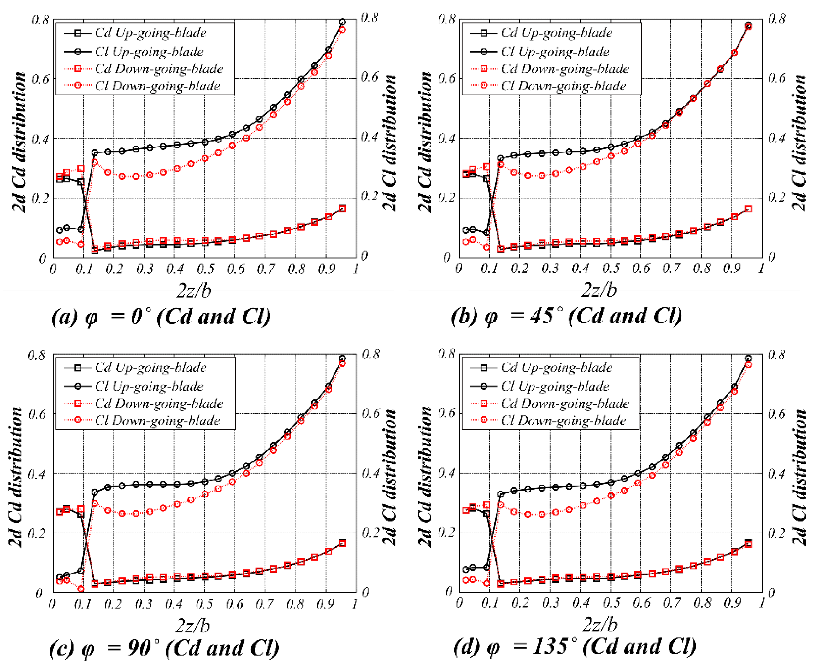
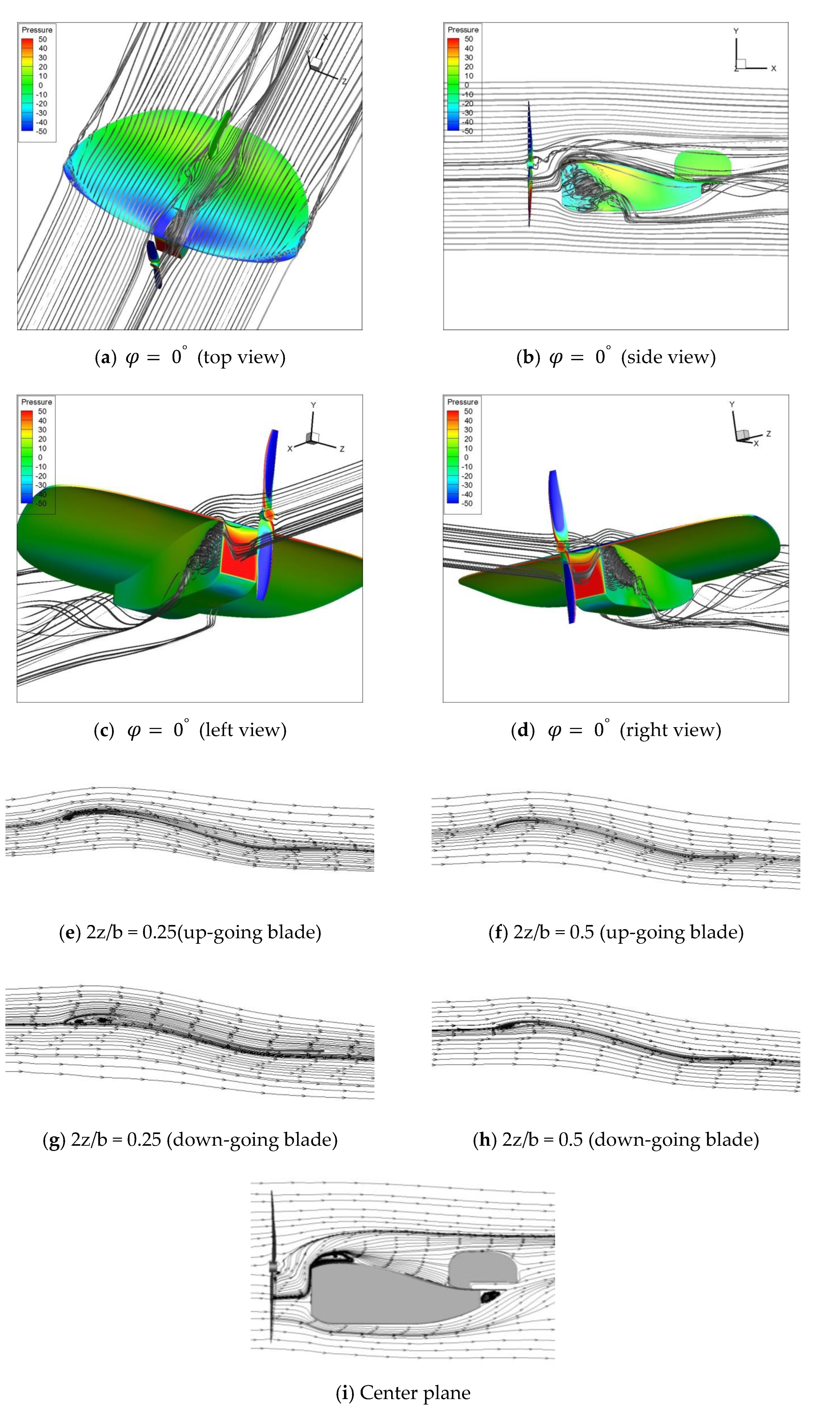
3.2. Propeller Slipstream Effect on the Flow Structure
4. Conclusions
Author Contributions
Funding
Institutional Review Board Statement
Informed Consent Statement
Data Availability Statement
Acknowledgments
Conflicts of Interest
References
- Shi, L.; Uy, C.; Huang, S.K.; Yang, Z.; Huang, G.P.; Wen, C.-Y. Experimental investigation on flow characteristics of a four-wing micro air vehicle. Int. J. Micro Air Veh. 2016, 8, 181–193. [Google Scholar] [CrossRef] [Green Version]
- Désert, T.; Moschetta, J.; Bézard, H. Numerical and experimental investigation of an airfoil design for a Martian micro rotorcraft. Int. J. Micro Air Veh. 2018, 10, 262–272. [Google Scholar] [CrossRef]
- De Wagter, C.; Karásek, M.; de Croon, G. Quad-thopter: Tailless flapping wing robot with four pairs of wings. Int. J. Micro Air Veh. 2018, 10, 244–253. [Google Scholar] [CrossRef] [Green Version]
- Lankford, J.; Mayo, D.; Chopra, I. Computational investigation of insect-based flapping wings for micro air vehicle applications. Int. J. Micro Air Veh. 2016, 8, 64–78. [Google Scholar] [CrossRef] [Green Version]
- Hassanalian, M.; Abdelkefi, A. Classifications, applications, and design challenges of drones: A review. Prog. Aerosp. Sci. 2017, 91, 99–131. [Google Scholar] [CrossRef]
- Hassanalian, M.; Abdelkefi, A. Design, manufacturing, and flight testing of a fixed wing micro air vehicle with Zimmerman planform. Meccanica 2017, 52, 1265–1282. [Google Scholar] [CrossRef]
- Mueller, T.J.; DeLaurier, J.D. Aerodynamics of Small Vehicles. Annu. Rev. Fluid Mech. 2003, 35, 89–111. [Google Scholar] [CrossRef]
- Chen, Z.J.; Qin, N.; Nowakowski, A.F. Three-Dimensional Laminar-Separation Bubble on a Cambered Thin Wing at Low Reynolds Numbers. J. Aircr. 2013, 50, 152–163. [Google Scholar] [CrossRef]
- Torres, G.E.; Mueller, T.J. Low-aspect-ratio aerodynamics at low reynolds numbers. AIAA J. 2004, 42, 865–873. [Google Scholar] [CrossRef]
- Mizoguchi, M.; Itoh, H. Effect of Aspect Ratio on Aerodynamic Characteristics at Low Reynolds Numbers. AIAA J. 2013, 51, 1631–1639. [Google Scholar] [CrossRef]
- Chen, Z.J.; Qin, N. Planform Effects for Low-Reynolds-Number Thin Wings with Positive and Reflex Cambers. J. Aircr. 2013, 50, 952–964. [Google Scholar] [CrossRef]
- Traub, L.W.; Botero, E.; Waghela, R.; Callahan, R.; Watson, A. Effect of Taper Ratio at Low Reynolds Number. J. Aircr. 2015, 52, 734–747. [Google Scholar] [CrossRef] [Green Version]
- Ikami, T.; Kanou, K.; Takahashi, K.; Fujita, K.; Nagai, H. Flow Field on Wing Surface with Control Surface in Propeller Slipstream at Low Reynolds Number. In Proceedings of the AIAA Scitech 2019 Forum, San Diego, CA, USA, 7–11 January 2019; American Institute of Aeronautics and Astronautics: Washington, DC, USA, 2019. [Google Scholar]
- Lyu, X.; Gu, H.; Zhou, J.; Li, Z.; Shen, S.; Zhang, F. Simulation and flight experiments of a quadrotor tail-sitter vertical take-off and landing unmanned aerial vehicle with wide flight envelope. Int. J. Micro Air Veh. 2018, 10, 303–317. [Google Scholar] [CrossRef] [Green Version]
- Marretta, R.M.A. Different Wings Flow Fields Interaction on the Wing-Propeller Coupling. J. Aircr. 1997, 34, 740–747. [Google Scholar] [CrossRef]
- Phillips, W.F.; Niewoehner, R.J. Effect of Propeller Torque on Minimum-Control Airspeed. J. Aircr. 2006, 43, 1393–1398. [Google Scholar] [CrossRef]
- Witkowski, D.P.; Lee, A.K.H.; Sullivan, J.P. Aerodynamic interaction between propellers and wings. J. Aircr. 1989, 26, 829–836. [Google Scholar] [CrossRef]
- Nickel, K.; Wohlfahrt, M. Tailless Aircraft in Theory and Practice; American Institute of Aeronautics and Astronautics: Washington, DC, USA, 1994. [Google Scholar]
- Menter, F.R.; Langtry, R.B.; Likki, S.R.; Suzen, Y.B.; Huang, P.G.; Volker, S. A Correction-Based Transition Model Using Local Variables- Part I: Model Formulation. J. Turbomach. 2006, 128, 413–422. [Google Scholar] [CrossRef]
- Colonia, S.; Leble, V.; Steijl, R.; Barakos, G. Assessment and Calibration of the γ-Equation Transition Model at Low Mach. AIAA J. 2017, 55, 1126–1139. [Google Scholar] [CrossRef] [Green Version]
- Suluksna, K.; Dechaumphai, P.; Juntasaro, E. Correlations for modeling transitional boundary layers under influences of freestream turbulence and pressure gradient. Int. J. Heat Fluid Flow 2009, 30, 66–75. [Google Scholar] [CrossRef]
- Benyahia, A.; Houdeville, R. Transition prediction in transonic turbine configurations using a correlation-based transport equation model. Int. J. Eng. Syst. Model. Simul. 2011, 3, 36. [Google Scholar] [CrossRef]
- Counsil, J.N.N.; Boulama, K.G. Low-Reynolds-Number Aerodynamic Performances of the NACA 0012 and Selig–Donovan 7003 Airfoils. J. Aircr. 2013, 50, 204–216. [Google Scholar] [CrossRef]
- Seyfert, C.; Krumbein, A. Evaluation of a Correlation-Based Transition Model and Comparison with the eN Method. J. Aircr. 2012, 49, 1765–1773. [Google Scholar] [CrossRef]
- Barth, T.; Jespersen, D. The design and application of upwind schemes on unstructured meshes. In Proceedings of the 27th Aerospace Sciences Meeting, Reno, NV, USA, 9–12 January 1989; American Institute of Aeronautics and Astronautics: Washington, DC, USA, 1989. [Google Scholar]
- Van Doormaal, J.P.; Raithby, G.D. Enhancedments of the SIMPLE Method for Predicting Incompressible Fluid Flows. Numer. Heat Transf. 1984, 7, 147–163. [Google Scholar] [CrossRef]
- Domino, S.P. Design-order, non-conformal low-Mach fluid algorithms using a hybrid CVFEM/DG approach. J. Comput. Phys. 2018, 359, 331–351. [Google Scholar] [CrossRef]
- Boller, C.; Kuo, C.M.; Qin, N. Biologically Inspired Shape Changing Aerodynamic Profiles and their Effect on Flight Performance of Future Aircraft. Adv. Sci. Technol. 2008, 56, 534–544. [Google Scholar]
- Brion, V.; Aki, M.; Shkarayev, S. Numerical simulation of low Reynolds number flows around micro air vehicles and comparison against wind tunnel data. In Proceedings of the 24th Applied Aerodynamics Conference, San Francisco, CA, USA, 5–8 June 2006. [Google Scholar]
- Ramamurti, R.; Sandberg, W.; Lohner, R. Simulation of the dynamic of micro air vehicles. In Proceedings of the 38th Aerodynamic Sciences Meeting & Exhibit, Reno, NV, USA, 10–13 January 2000. [Google Scholar]


| Case | Grid Size | CL | CD | |
|---|---|---|---|---|
| Model 1 | G1 | 190 × 135 × 60 | 0.1744 | 0.01913 |
| G2 | 220 × 165 × 90 | 0.1775 | 0.02068 | |
| G3 | 250 × 195 × 120 | 0.1781 | 0.02052 | |
| Model 2 | G1 | 190 × 135 × 60 | 0.1899 | 0.01890 |
| G2 | 220 × 165 × 90 | 0.1900 | 0.01877 | |
| G3 | 250 × 195 × 120 | 0.1901 | 0.01879 | |
| Experiment [1] | NA | 0.1906 ± 0.02 | 0.0220 ± 0.003 |
| MAV model | ) | ) | ) | ) | ) |
| 0.068(31.7%) | 0.059(26.6%) | 0.216(97.6%) | 0.021(9.49%) | 2e−3(0.93%) |
Publisher’s Note: MDPI stays neutral with regard to jurisdictional claims in published maps and institutional affiliations. |
© 2022 by the authors. Licensee MDPI, Basel, Switzerland. This article is an open access article distributed under the terms and conditions of the Creative Commons Attribution (CC BY) license (https://creativecommons.org/licenses/by/4.0/).
Share and Cite
Chen, Z.; Yang, F. Propeller Slipstream Effect on Aerodynamic Characteristics of Micro Air Vehicle at Low Reynolds Number. Appl. Sci. 2022, 12, 4092. https://doi.org/10.3390/app12084092
Chen Z, Yang F. Propeller Slipstream Effect on Aerodynamic Characteristics of Micro Air Vehicle at Low Reynolds Number. Applied Sciences. 2022; 12(8):4092. https://doi.org/10.3390/app12084092
Chicago/Turabian StyleChen, Zhaolin, and Fan Yang. 2022. "Propeller Slipstream Effect on Aerodynamic Characteristics of Micro Air Vehicle at Low Reynolds Number" Applied Sciences 12, no. 8: 4092. https://doi.org/10.3390/app12084092
APA StyleChen, Z., & Yang, F. (2022). Propeller Slipstream Effect on Aerodynamic Characteristics of Micro Air Vehicle at Low Reynolds Number. Applied Sciences, 12(8), 4092. https://doi.org/10.3390/app12084092